https://www.researchgate.net/publication/228699590
Performance evaluation of the
sequential track initiation
schemes with 3D position and
Doppler velocity measurements
Article in Progress In Electromagnetics Research B · January 2009
DOI: 10.2528/PIERB09072306 CITATIONS
6
READS33
4 authors, including: Some of the authors of this publication are also working on these related projects: MODELING OF STRUCTURAL PROPERTIES OF ANOMALIES AND DISTURBANCES FOR THE IONOSPHERE OVER TURKEYView project Bayesian RFS Estimators
View project F. Arikan Hacettepe University 111 PUBLICATIONS 633 CITATIONS SEE PROFILE Orhan Arikan Bilkent University 58 PUBLICATIONS 230 CITATIONS SEE PROFILE
All content following this page was uploaded by Faruk Kural on 04 October 2017.
PERFORMANCE EVALUATION OF THE SEQUENTIAL TRACK INITIATION SCHEMES WITH 3D POSITION AND DOPPLER VELOCITY MEASUREMENTS
F. Kural
Meteksan Defence Ind. Inc. Ankara Cyberpark
Bilkent University Ankara, Turkey F. Arıkan
Department of Electrical and Electronics Engineering Hacettepe University
Beytepe, Ankara, Turkey O. Arıkan
Department of Electrical and Electronics Engineering Bilkent University
Bilkent, Ankara, Turkey M. Efe
Department of Electronics Engineering Ankara University
Tandogan, Ankara, Turkey
Abstract—This study investigates the effect of incorporating Doppler velocity measurements into the most commonly used sequential track initiation schemes, the rule and logic based schemes. The measurement set has been expanded from range and azimuth to include elevation and Doppler velocity. Unlike previous studies, elevation and Doppler measurements have also been included in the analytical evaluation of the false track initiation probability. Performance improvement obtained by employing Doppler measurements has been demonstrated through simulations in terms of false track initiation probability and true track initiation probability. Receiver Operating Characteristics
and System Operating Characteristics have also been utilized in performance evaluation. Analytical derivations and simulations have revealed that using Doppler velocity measurements along with 3D position measurements while initiating tracks in clutter leads to significant decrease in false track initiation probability while providing an acceptable level of true track initiation probability. Simulation results have also shown that inclusion of Doppler measurements has reduced the required time for track initiation, resulting in faster track initiation.
1. INTRODUCTION
The problem of target tracking has been an important issue of signal processing for many years, and a variety of tracking methods have been recommended in literature [1–8]. Track initiation (TI) is a fundamental and essential part of target tracking process in real life tracking applications, and the tracking performance in cluttered environment heavily relies on the success of TI and measurement-to-track association algorithms. In a radar measurement-to-tracking system, extracted measurements from detections are transferred to the target tracking module with a transfer rate allowed by the radar. Measurements are first fed into measurement-to-track association unit which correlates them with the targets being tracked. Measurements which have not been correlated with any of the registered tracks are assumed to have originated from new potential targets, and they are directed to the TI unit.
Performance of the employed TI scheme plays an important role in the performance of the tracking module in real life systems. When the TI unit fails to initiate tracks from the existing targets, radar may miss the opportunity to track and identify the potential targets. On the other hand, in case where false tracks are initiated, limited radar resource is wasted, and the computational burden is increased to maintain non-existing targets, resulting in the reduction of the number of true targets to be tracked. Thus, it is very critical for TI to correctly initiate tracks from real targets as fast as possible. Furthermore, TI should also discard undesired measurements specifically originated from clutter which is from the list of measurements to be used to initiate a track. Hence, a statistically successful TI should be able to set its True Track Initiation Probability (TTIP) to an acceptable level while keeping the False Track Initiation Probability (FTIP) as low as possible.
schemes. The sequential schemes, also called the information based schemes, involve the processing of a sequence of measurements received during consecutive radar scans. Measurements taken from N time scans are processed sequentially in a time-window trying to reach a specified value for the number of detections in order to declare a track. For the batch schemes, measurements from the past N scans are processed simultaneously to determine feasible target trajectories. The N scans of data are treated as an image, and the tracks are initiated if some curves (usually straight lines) are detected [9]. Rule and logic based schemes are sequential schemes, and Hough Transform (HT) and the modified HT are batch schemes [9–12]. Batch schemes are less preferred in practical tracking systems due to their heavier computational burden and slower process.
While TI is of great importance for a real life tracking system, limits of its performance can only be obtained through time-consuming and computationally expensive simulations. Thus, any means for analytically evaluating the performance of TI schemes would be of great help while designing a tracking system for real life applications. Unfortunately, studies on analytical performance of TI schemes are very rare and limited [9, 10, 13–15]. In these studies, only two dimensional (2D) position measurements, range and azimuth, are considered. However, the major discriminant of clutter from a desired target with relatively higher velocities would be the Doppler velocity measurement [16–22]. Recent studies [23, 24] have reported that incorporating Doppler velocity measurements into TI schemes considerably decreases the number of confirmed false tracks per scan. The number of confirmed true tracks per scan is the same for both position only and position plus Doppler velocity measurement cases. Furthermore, the results presented in [23, 24] indicate that, in track maintenance after initiation, a substantial improvement to the tracking performance has been achieved in terms of the number of the confirmed true tracks by incorporating Doppler velocity measurements.
Although many Phased Array Radars (PAR) are capable of providing additional return information such as elevation and Doppler velocity, to the authors knowledge, there has not been any study in the open literature where these additional measurements have been included in the analysis of TI schemes.
Therefore, in this paper, we aim to develop analytical means for evaluating performance of the two most commonly used sequential TI schemes, the rule based and logic based TI schemes when the Doppler measurement is included in the measurement set. Also, since the outcomes of the analytical studies dealing with 2D measurements are not easily applicable to cases where the measurements are taken in
3D, we have included elevation and Doppler velocity information in 2D position measurements and produced analytical performance measures for this new measurement set.
The performance analysis of the TI schemes has been done in terms of FTIP and TTIP, where FTIP is defined as the probability of initiating a track from false alarms or using measurements originated from clutter whereas TTIP is defined as the probability of initiating a track that is not a false track. In essence, TTIP can be seen as the track initiation probability, and it can be calculated/simulated relatively easily based on the single dwell true detection probability, PD. On the other hand, analytical calculation and/or simulation, thus the evaluation, of FTIP is more complicated [13]. In this study, analytical evaluation of FTIP with a measurement set containing 3D position and Doppler measurements has been carried out for the first time. Receiver Operating Characteristics (ROC) have also been employed in the performance evaluation of the TI schemes considered in this study. Moreover, depending on the obtained ROC curve of the generic PAR considered in this study, System Operating Characteristics (SOC) curves have been obtained which are very critical for the assessment of the performance of the TI scheme of the tracking system employed in PAR.
The outline of the paper is as follows. Section 2 gives a brief description of the two mostly used TI schemes and the analytical derivations of FTIP for position only and position plus Doppler velocity measurements. A discussion about TTIP for position and Doppler velocity measurements is also presented. In Section 3, results of computer simulations that have been performed to verify the derived analytical expressions are given. Section 4 presents concluding remarks and discusses the usefulness of including Doppler velocity measurements to increase the performance of TI schemes.
2. TRACK INITIATION SCHEMES
Rule based [10] and logic based [9, 10, 13–15] TI schemes are the most commonly used sequential TI schemes in radar tracking systems. The following subsections outline these schemes along with analytical evaluation of FTIP for 3D position only measurements, the expansion of the analytical evaluation to 3D position and Doppler measurements for the mentioned schemes.
2.1. Rule-based TI Scheme with Position Only Measurements
The rule based scheme uses the constraints, i.e., minimum and maximum values on velocity and acceleration as rules in order to reduce the number of tracks to be initiated. Let sampling interval, ts, be defined as the constant period of sending all extracted measurements in the search region to the tracking unit. In general, PARs utilize a varying sampling interval depending on the estimated dynamics of the tracked target(s). However, during TI a constant sampling period can be assumed [25, 26]. In the rule-based scheme, expected minimum and maximum velocity values about the targets to be tracked define a velocity gate given by (1), and absolute value of the velocity is computed from the position measurements [10]
υmin≤ k rj,i+1(1 : 3) − rk,i(1 : 3) k/ts≤ υmax (1) where i is the sampling time index with i = 1, 2, . . . , M − 1; M is the number of sampling events (scans) required for initiation; rk,i = [ xk,i yk,i zk,i υk,i ]T is the kth measurement vector containing Cartesian position and Doppler velocity measurements at the ith sampling time; rk,i(1 : 3) = [ xk,i yk,i zk,i ]T, [.]T denotes transpose operator; k . k is the L2 vector norm operator; υmin, υmax (υmax > υmin ≥ 0) denote the minimum and the maximum velocity threshold values for the targets of interest, respectively. Hence, if the computed speed is smaller/larger than the expected speed of the slowest/fastest target of interest, then the measurement is deemed not to have originated from a potential target. If more than one measurement falls inside the gate at the second scan, then velocity gating is carried out with each gated measurement with no specific order, and the first measurement that satisfies the test is used for association. Similar to the computed velocity, the estimated acceleration is also gated as it must be below the maximum allowed acceleration value, thus an acceleration gate is given by (2) is formed [10]
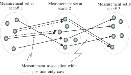
k(rj,i+1(1 : 3)−rk,i(1 : 3))/ts−(rk,i(1 : 3)−rl,i−1(1 : 3))/tsk ≤ amaxts (2) where amax (amax > 0) denotes the maximum acceleration level of the targets. In rule based TI scheme, a potential track is formed at (i + 1)th scan whenever the measurements satisfy both of the rules given by (1) and (2). If more than one measurement falls inside the gate at the second scan, then velocity gating is carried out with each gated measurement with no specific order, and the first measurement that satisfies the test is used for association. Fig. 1 presents an illustrative example of measurement association process with position only and position plus Doppler velocity measurements in
1 scan# at set Measurement scan# at set Measurement scan# at set Measurement 2 3
Measurement association with: ____ position only case
--- position plus Doppler velocity case
Figure 1. Diagram of measurement matching at successive scans with position only and position plus Doppler velocity cases.
case of the existence of single target scenario. Each ellipse contains 3D (or 4D for Doppler velocity measurement case) radar measurement set for each scan. Filled circles in the ellipses are used to depict measurements extracted for each scan. Arrows between successive scans indicate associated measurement pairs where solid and dashed arrows show the use of position measurements only and position plus Doppler measurements for association respectively. When additional Doppler gating is applied, only two associations are made going into the second scan which is reduced to one association in the third scan in comparison to four associations in both scans with position only case. At the end of the third scan, a true track is initiated for both cases. However, in position only measurement case, three false tracks are also initiated. Therefore, the number of false associations can be reduced through incorporating Doppler velocity measurements into the initiation procedure. In rule based track initiation, every potential track that passes the tests defined by (1) and (2) for a predefined number of scans is registered as a new track. Otherwise, the process is terminated, and no track is formed.
2.1.1. FTIP Analysis for the Rule-based TI Scheme with Position Only Measurements
Clutter and false alarm based undesired measurements degrade the performance of tracking system by mainly increasing FTIP. A
statistically successful TI process should set the TTIP to an acceptable level while keeping FTIP as low as possible. In this subsection, the analysis, that was carried out for 2D measurements [10], e.g., range and azimuth, is expanded to include the elevation measurements as well.
Starting with the computation of FTIP for the rule-based TI scheme, let the probability of having an undesired measurement inside the gate defined by (1) and the number of effective resolution cells for a single dwell be pi (i ≥ 2) and ζ, respectively. Here, ζ = [[(Rmax− Rmin)/∆R]] where Rmax and Rmin are the maximum unambiguous and minimum range of the PAR, respectively; ∆R is the resolution cell size of the PAR; [[.]] is the round to the nearest integer operator. Let the total number of beams assigned for the search process be Nb, and the probability mass function of the number of undesired returns in these Nbζ cells is Poisson distributed [1]. Therefore, the expected number of undesired measurements in the search region can be calculated as N = [[NbζPF A where PF A is detector’s false alarm probability per resolution cell, and [[. is the floor function that gives the largest integer less than or equal to its argument. At the 2nd sampling time, probability of having at least one undesired measurement inside the gate given by (1) is expressed as [10, 27]:
PF,2 = 1 − exp(−N p2) = 1 − exp(−[[(NbζPF A)p2) (3) It is a common mathematical model that Cartesian distribution of the undesired measurements is uniform in the search region which is based on two assumptions [1]. The first one is that the events of detection in each cell are independent of each other, and the probability of having a measurement in any cell is equal. The second one is that the probability of such a detection, which is a false alarm, is PF A in each cell. Then using classical definition of probability [27], the probability that a clutter or false alarm based position only measurement at the 2nd sampling time falls into the gate defined by (1), p2 is calculated as p2 = V2/Vs. Here, Vs is the total volume of the search region, and V2 = 43π
¡
R32− R31¢ is the volume of the velocity gate defined by (1) where R1 = υmints and R2 = υmaxts [10]. It has been reported that fluctuation of many complex targets is successfully represented by the Swerling models [28]. Through the known relationships between PF A and PD, which include signal-to-noise ratio and detector threshold for all the Swerling fluctuation types, FTIP is also related to the PD, hence it is possible to form a relationship between signal and data processing units. Also, the results can be easily extended to any other given expanded-Swerling or Non-Swerling fluctuation probability distribution [29–32]. Continuing with the TI process, any measurement extracted at the 3rd sampling time must comply with the constraints
(and their derived forms) given in Appendix A. At the 3rd sampling time, probability of having at least one undesired measurement obeying the constraints can be calculated similar to (3) as:
PF,3= 1 − exp(−[[(NbζPF A)p3) (4) In (4), given the existence of a measurement pair passing the velocity gating defined by (1) from the 1st and 2nd sampling times, p3 is the probability that a clutter or false alarm based position only measurement conforms to the constraints presented in Appendix A. Although the derivation of p3 is one of the main contributions of this study, it is detailed in Appendix A for the sake of continuity. Since both velocity and acceleration gatings are also applied at the 4th sampling time, PF,4 is chosen approximately equal to PF,3 [10]. In this study, total number of sampling times to initiate a track has been chosen as M = 4 which is a widely used number of total sampling times for initiation with the considerations of complexity and accuracy [10, 13, 14]. Since false measurements are assumed to be independent from scan to scan [1], it is viable to assume that the FTIP at each sampling time is independent for the M sampling TI [10]; the overall FTIP is then given by PF T IP = PF,2PF,3PF,4. The following subsection presents the rule-based TI scheme with 3D position and Doppler velocity measurements.
2.2. Rule-based TI Scheme with Position and Doppler Velocity Measurements
In this subsection, the rule-based TI scheme with additional Doppler velocity measurements is investigated. Define tth vector pairs as rt,i and rt,i+1 which have successfully passed position only based velocity and acceleration tests at the ith and (i + 1)th sampling times, where i = 1, 2, 3 for the velocity test and i = 2, 3 for the acceleration test. Since acceleration can only be estimated starting at the end of the second sampling time, the counter starts at 2 for the acceleration test. Then, additional tests for the Doppler velocity measurements to be carried out are given below.
( υ
min≤ |rt,i+1(4)| ≤ υmax
∩ |rt,i+1(4) − rt,i(4)|/ts≤ amax ∩ (rt,i+1(4) rt,i(4)) ≥ ξυ
)
(5) where i = 1, 2, 3. In (5), additional tests are applied to the measurements which have successfully passed the position only based tests. The first two tests are based on the absolute value of Doppler velocity measurement, and the final one uses the direction of Doppler velocity measurement [21]. Firstly, the absolute value of
the Doppler velocity measurement is tested to see whether it falls into the velocity gate†. Then, absolute value of the acceleration, which has been calculated as the difference of Doppler velocity measurements obtained at successive sampling times, is thresholded against the maximum acceleration level. Finally, considering the fact that a target cannot move in the opposite direction to its normal course in a short time period, an additional lower limit threshold, based on the minimum velocity change of the targets during a sampling interval, ξυ = −(amints)2, is applied, where amin is the expected minimum acceleration level of the target during a maneuver. Herein, due to the possible different signs of Doppler velocity measurements between successive samplings, the negative sign is used. Additional tests aim to take advantage of the expanded measurement vector and remove undesired measurements which have relatively less Doppler velocities than a complex target of interest.
2.2.1. FTIP Analysis of the Rule-based TI Scheme with Position and Doppler Velocity Measurements
In this subsection, analytical evaluation of FTIP using Doppler velocity measurement along with 3D position measurements is derived. In cases where Doppler velocity measurements are available at the ith sampling time, the probability of having an undesired measurement inside the velocity (i = 1, 2, 3) and acceleration gates (i = 2, 3) is defined as:
pDi = p∆ i∩P ((υmin≤ |υ| ≤ υmax) ∩ (|υ − υp|/ts≤ amax) ∩ (υυp≥ ξυ)) (6) where, P (.) is the probability of the event inside the brackets; υ is the Doppler velocity measurement at the current sampling time; υp is the Doppler velocity measurement from the preceding sampling time. Since the FTIP is of interest here, it is assumed that the Doppler measurements have originated from clutter or false alarm. It should be noted that the first probability, pi, is based on position only measurements, and the rest of the event in P () employs the extracted Doppler velocity measurements directly. Thus, pi and P () can be considered statistically independent. Since clutter based false Doppler detections υ and υp are assumed uncorrelated, occurrence of the first event in P (.) in (6) most probably does not affect the occurrence of the second event in P (.) of (6). Certainly, this is not exactly a marginal or absolute independency, and the events may be assumed to be joint events with a multivariate distribution which † Note that targets can have zero Doppler velocity in their trajectories, which is out of
the interval defined by (1) and will reduce TTIP. However, this will also cause significant decrease in FTIP.
cannot be calculated uniquely using the marginal distributions of the events in P (.) only. Therefore, in order to be able to calculate the overall FTIP, a mild ‘independency of the events’ assumption is made. Furthermore, this assumption is tested with computationally intensive and time consuming simulations which are in agreement with the analysis as to be presented in Section 3. The difference between analytical and simulated results can be considered due to the fact that the absolute independency between the events including Doppler velocity measurements cannot be maintained. In addition, similar assumptions which were similarly proven with the simulations were made e.g., in [10] in order to be able to calculate the overall FTIP. Therefore, pD i is expressed as: pDi = piS1S2S3 (7) where S1 = P (υ∆ min≤ |υ| ≤ υmax) (8) S2 = P (|υ − υ∆ p|/ts≤ amax) (9) S3 = P (υυ∆ p ≥ ξυ) (10)
Assume that the Doppler velocity of the undesired measurements is uniformly distributed between expected minimum and maximum velocities, then probability density function of the undesired bipolar Doppler velocity measurements is:
f (υ) =
½ 1
2υcmax −υcmax ≤ υ ≤ υcmax
0 otherwise (11)
where υcmax is the assumed maximum Doppler velocity of undesired
measurements. Hence, S1 = υZmax υmin f (|υ|) d (|υ|) = ³ 1 − υmin υcmax ´
υmin < υcmax < υmax
³
υmax−υmin
υcmax ´
υmin < υmax< υcmax
(12) The probability density function of random variable, ∆υ = υ − υp, in (9) is calculated as: f (∆υ) = ( 1 2υcmax ³ 1 −2υ|∆υ| cmax ´ −2υcmax ≤ ∆υ ≤ 2υcmax 0 otherwise (13) and f (|∆υ|) = ( 1 υcmax ³ 1 −2υ|∆υ| cmax ´ 0 ≤ |∆υ| ≤ 2υcmax 0 otherwise (14)
Therefore, S2= P (|∆υ| ≤ amaxts) is: S2 = amaxZ ts 0 f (|∆υ|) d (|∆υ|) = ( ³ amaxts υcmax ´ ³ 1 − amaxts 4υcmax ´ amaxts < 2υcmax 1 otherwise (15)
As it can be seen from (15), if amaxts ≥ 2υcmax, then S2 = 1, i.e.,
the contribution from inclusion of the Doppler velocity measurement disappears, resulting in the increased FTIP.
Using the multiplication rule of two random variables [27], S3 is calculated as: S3= υ2 cmax Z ξυ µ ln µ υ2 cmax |z| ¶Á¡ 2υ2cmax¢ ¶ dz = 0.5 −2υξυ2 cmax ³ 1 + ln ³ −υ2 cmax ξυ ´´ ξυ< 0 0.5 ξυ= 0 0.5 −2υξυ2 cmax ³ 1 + ln ³ υ2 cmax ξυ ´´ ξυ> 0 (16)
Note that in order for S3 to contribute to the reduction in FTIP, it is required that S3< 1 in (16), which in return requires |ξυ| ≤ υ2
cmax.
Finally, substituting (12), (15) and (16) into (7) for i = 2, PD
F,2 is obtained for υmin < υcmax < υmax, −υc2max < ξυ < 0 and
amaxts< 2υcmax as:
PF,2D = 1−exp −[[(NbζPF A)p2 ³ 1− υmin υcmax ´³ amaxts υcmax ´³ 1−amaxts 4υcmax ´ × ³ 0.5−2υξυ2 cmax ³ 1 + ln ³ −υ2 cmax ξυ ´´´ (17) At the 3rd sampling time, probability, which any undesired measurement falling into both velocity and acceleration gates when Doppler velocity measurements are available, pD
3 is similarly calculated as: pD3 = p3S1S2S3 (18) Then, PF,3D = 1−exp −[[(NbζPF A)p3 ³ 1− υmin υcmax ´³ amaxts υcmax ´³ 1−amaxts 4υcmax ´ × ³ 0.5 − 2υξυ2 cmax ³ 1 + ln ³ −υ2 cmax ξυ ´´´ (19) Since both velocity and acceleration gating are applied at the 4th sampling time, PF,4D is chosen approximately equal to PF,3D , and the
overall FTIP for TI is calculated as PD
F T IP = PF,2D PF,3D PF,4D . The following subsection gives the FTIP analysis of logic-based TI scheme for both position only and position plus Doppler velocity cases. 2.3. Logic-based TI Scheme and FTIP Analysis with Position Only Measurements
The logic based initiation scheme uses prediction and gating in order to identify potential measurements to be used in TI. The initiation procedure of the logic and rule based schemes are identical for the first two sampling times. However, the main difference between the two schemes is that, in the logic-based scheme, which is also known as the “m out of n” TI, following the second detection, a gate is set up for the next sampling time, and detection has to be made within this gate [9, 10, 13–15]. If the conditions of this gating are satisfied, then other gates are installed for the following sampling intervals based on the considered target dynamics, and a detection has to be made in m out of the next n sampling times in the equivalent gates.
Initiation starts with the measurements acquired in the first two sampling intervals. Velocity is then calculated from this measurement pair and put through the velocity gating defined by (1). If the velocity gating is successful then a preliminary track is registered. Next, a position prediction based on the measurement at the current sampling interval for the given gate and a velocity estimation is made for the following sampling interval using
ˆri+2= rj,i+1(1 : 3) + ((rj,i+1(1 : 3) − rk,i(1 : 3)) /ts) ts (20) At the next sampling time, an acceptance gate with the radius of r0 is set up around ˆri+2. Any measurement falling in this gate will extend the potential track. At the following sampling interval, both velocity and acceleration gates are set up. Finally, a position prediction is made through (21).
ˆri+3 = rl,i+2(1 : 3) + k(rl,i+2(1 : 3) − rj,i+1(1 : 3))/tsk ts +0.5 (((rl,i+2(1 : 3) − rj,i+1(1 : 3)) /ts
− (rj,i+1(1 : 3) − rk,i(1 : 3)) /ts) /ts) t2s (21) If no measurement falls in the gate, the preliminary track gets terminated. The procedure defined by (21) is an M out of N type track initiation, and although different combinations are possible, which changes the PD, with M out of N type track initiation, (21) suggests that a track is initiated only if associations are made in 3 successive scans. The measurements that are not associated with the potential tracks are assumed to have originated from new tracks, and all the
procedures defined previously are repeated for M sampling times. If more than one measurement are inside the gate, the measurement that has the smallest distance to the predicted position is used.
The TI procedure for the first two sampling times is the same as the rule-based scheme. Therefore, they share the same FTIP. At the next sampling times, a fixed volume gating is used where the volume of the gate is Vi = 43πr03 and 3 ≤ i ≤ M . Hence, the probability pi is calculated as pi = Vi/Vs and for M = 4, overall FTIP is PF T IP = PF,2PF,3PF,4 where PF,i = 1 − exp(−[[(NbζPF A)pi). In the next subsection, incorporating Doppler velocity into the logic-based TI scheme is analytically expressed.
2.4. Logic-based TI Scheme and FTIP Analysis with Position and Doppler Velocity Measurements
Here, the logic-based TI scheme with additional Doppler velocity measurements is investigated in an analytical manner for the first time. At the ith sampling time, define a measurement vector ˆrl,ifalling in the pre-set gate of the potential registered track which extends from the (i − 1)th sampling time. For this measurement, let its pair belonging to the (i − 1)th sampling time be ˆrm,i−1. They are put through the Doppler velocity measurement based tests given below (i = 2, 3, 4).
(
υmin≤ |ˆrl,i(4)| ≤ υmax
∩ |ˆrl,i(4) − ˆrm,i−1(4)|/ts≤ amax ∩ (ˆrl,i(4) ˆrm,i−1(4)) ≥ ξυ
)
(22) FTIP of the logic-based TI scheme with position and Doppler velocity measurements is still the multiplication of the marginal FTIPs obtained at different sampling times, i.e., PD
F T IP = PF,2D PF,3D PF,4D where PD
F,i = PF,iS1S2S3. The proceeding subsection summarizes the calculation of the TTIPs for both TI methods.
2.5. TTIP Calculation of the TI Schemes
TTIP is calculated as a function of the PD and the measurement accuracy for the specific target motion models [10, 13, 14]. In [10], TTIP was taken nearly unity as for range measurements with measurement noise of 200 m standard deviation at unit PD for both TI methods. When Doppler velocity measurements are used for TI process, due to the additional tests, TTIP was shown to be reduced [20– 22]. Thus, in the next section, Monte Carlo simulations have been performed for the target scenarios in order to obtain TTIP.
3. SIMULATION RESULTS
This section presents the evaluation results of the derived analytical expressions through simulations. In this section, both the radar model and target scenarios are taken from the benchmark problem [33]. The selected PAR is a multi-functional generic radar with search and tracking functions. It is an X-band radar having half power beamwidths of 1.5◦ in both azimuth, θ
3 dB, and elevation, φ3 dB. The scanned sector for TI is chosen from θ1= −60◦ to θ2 = 60◦ in azimuth and from φ1 = 2◦ to φ2= 80◦ in elevation.
Since the radar beam can be steered electronically, the sampling interval can be decreased to an acceptable value for track maintenance depending on the maneuvering capability of the targets. In this study, the sampling interval, ts, is fixed at 2 s for TI.
Taking into account that the shape of the beams is an elliptic cone having height of Rmax, semi-major axis a = 0.5Rmaxθ3 dB and semi-minor axis b = 0.5Rmaxφ3 dB, the volume covered by a beam is calculated as Vb = πRmaxab/3 = 350.5 km3 where Rmax is 125 km. Since the number of beams with no overlapping in the region Nb = [[((θ2− θ1) (φ2− φ1)/(θ3 dBφ3 dB)) = 4, 160, total search volume is Vs= VbNb = 1.46 × 10⁶km3.
For the calculated total SNR value of 8.9 dB at Rmax with 16 integrated pulses, the worst case measurement accuracies can be approximated through the closed-form expressions given in [2], as 20 m in range, 1.7 mrad in both azimuth and elevation and 40 m/s in Doppler velocity after resolving Doppler ambiguity. Note that, although measurements for the benchmark problem do not include Doppler velocity, here Doppler velocity measurements were generated first utilizing the position and velocity values in Cartesian coordinates as defined in [22] then adding uniform distributed measurement noise with the standard deviation of the calculated accuracy defined above. Parameters for TI are selected by taking into account the motion characteristics of the benchmark targets. Since the targets have distinct maximum acceleration values, amax is a critical parameter, thus, a set of amax has been employed, which is chosen as 31; 39; 42; 58; 68; 70 m/s2. The minimum velocity threshold value based on the minimum acceleration level amin, of the benchmark targets during maneuver is calculated as υmin = amints = 40 m/s. The threshold value, ξυ, used for velocity testing in TI is ξυ = −υ∆ 2min = −1.6 × 10³. The maximum velocity threshold is taken as υ
max =
1000 m/s regarding the benchmark targets.
For a fair analysis, the maximum value for the Doppler velocity of clutter is realistically chosen with the similar target Doppler velocities
as υcmax = 150 m/s.
3.1. Simulation Results for TTIP
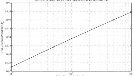
Firstly, simulations to estimate TTIP will be considered. System requirement about TTIP is preset as PT T I ≥ 0.70 when M = 4. For the logic-based TI scheme, radius parameter has been chosen as r0 = 500 m to meet the minimum TTIP requirement. Total number of Monte Carlo run used in the simulations is 5, 000 in an attempt to yield unbiased TTIP results. Employing these parameters, Monte Carlo simulations for the benchmark targets have been performed to examine the TTIP performance for both TI schemes. In simulations, 3D polar measurements are produced for the selected benchmark target only if a uniformly distributed ([0, 1]) random variable is less than the PD for that particular sampling interval. Through this procedure miss detections are modeled. When a target originated detection based on a given PD is declared, a uniform distributed measurement noise vector in which each component has a standard deviation with the corresponding calculated accuracy is added onto the true polar measurement. The noisy polar measurements are then converted to 3D Cartesian coordinates using standard conversion techniques. For Swerling-3 type benchmark targets considered in this study, a closed form expression, which interrelates PF A and PD, is given in [2]. So, a set of false alarm probabilities has been chosen by taking the number of effective range resolution cells into consideration, as 1 × 10⁻⁶; 5 × 10⁻⁶; 1 × 10⁻⁵; 5 × 10⁻⁵ and 1 × 10⁻⁴ per resolution cell in order to calculate PD. Fig. 2 depicts the ROC curve calculated for the selected PF A and the corresponding PD values when the single pulse SNR value is 8.9 dB at Rmax/2. Since it relates the PF A to PD, which is also used in the TI process, the ROC curve is crucial for the performance evaluation of the TI methods.
If all the conditions defined for the TI methods are satisfied at the end of M th sampling time (M = 4), a track is initiated, and the number of correctly initiated tracks for a single run is taken as 1. TTIP estimations for amax= 70 m/s2 are given in Table 1. Simulation results have revealed that increasing M yields a reduction in the TTIP [22].
Results indicate that when Doppler velocity measurement is used in the TI process, due to the additional tests, reduction in TTIP varies depending on the maneuver capability and Doppler velocity profile of the benchmark targets. As it can be seen from Table 1, average percentage reduction in TTIP for position and Doppler velocity case due to the additional tests considering all the benchmark targets is approximately 6% for both TI methods. However, despite the decline in TTIP, the system requirement PT T I ≥ 0.70 is still met, even when
10-6 10-5 10-4 0.92 0.925 0.93 0.935 0.94 0.945 0.95 0.955 0.96
False Alarm Probability, P
FA
True Detection Probability, P
D
Receiver Operating Characteristics (ROC) Curve of the Detection Unit
Figure 2. Receiver Operating Characteristics (ROC) curve of the detection unit.
Table 1. TTIP values of the TI methods (RB: rule-based TI, LB: logic-based TI, PO: position only measurements, PD: position and Doppler velocity measurements, Red.%: percentage of reduction in TTIP due to Doppler velocity inclusion).
Target No RB-PO RB-PD Red.% LB-PO LB-PD Red.%
1 0.83 0.76 8.4 0.85 0.79 7.0 2 0.81 0.81 0.0 0.81 0.81 0.0 3 0.81 0.81 0.0 0.84 0.84 0.0 4 0.83 0.70 15.6 0.83 0.70 15.6 5 0.78 0.77 1.2 0.85 0.83 2.3 6 0.79 0.70 11.3 0.82 0.73 10.9
the Doppler velocity measurement is used. Furthermore, logic-based TI scheme is superior to its competitor in terms of TTIP values. 3.2. Simulation Results for FTIP
Analytical expressions obtained for FTIPs have been verified through simulations for various and widely used levels of false alarm probability. For this set of simulations the range resolution has been taken as 150 m, which results in ζ = 832 effective range resolution cells per dwell. Therefore, total number of range resolution cells for the search
region is Nbζ = 3, 461, 120. PF A values given in the preceding subsection, therefore, yield, on average, 3; 17; 34; 172 and 345 undesired measurements in the search region of interest, N , respectively. For M = 4 and varying PF A from 1 × 10⁻⁵ to 1 × 10⁻⁶, uniformly distributed random variables in Cartesian coordinates are generated such that they fall into the coverage volume of the PAR. Furthermore, values of Doppler velocity attached to the undesired measurements are drawn from the uniformly distributed random variables between −υcmax and υcmax. Then, simulations have been performed for the PF A
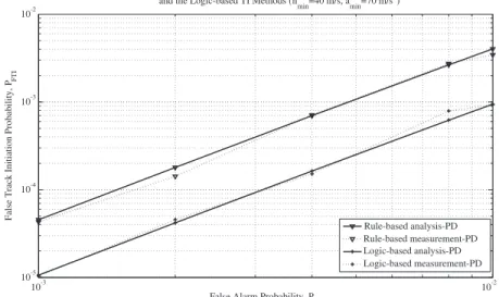
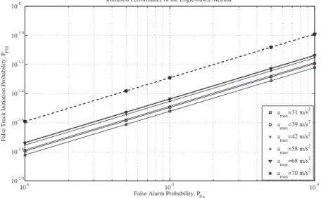
values of 1 × 10⁻³, 2 × 10⁻³, 4 × 10⁻³, 8 × 10⁻³ and 1 × 10⁻² for M = 3 and amax = 70 m/s2 due to the processing power limitations of the simulation environment. As a comparison, the analytical and simulated results given in Fig. 3 for the rule- and logic-based schemes are very close to each other. Since the simulated results are nearly in good agreement with the analytical results for M = 3, no simulations were performed for M = 4. Then, all the results obtained analytically given in Figs. 4–7 have been obtained for M = 4. Fig. 4 presents FTIP performance of the rule-based TI scheme for position only and position plus Doppler velocity measurements. As it can be seen in Fig. 4, when the PF A and amax get larger so does the PF T I due to increasing number of samples satisfying velocity and acceleration tests.
10-3 10-2
10-5 10-4 10-3 10-2
False Alarm Probability, P
FA
False Track Initiation Probability, P
FTI
Comparison of Analytical and Simulation Results for the Rule-based and the Logic-based TI Methods (n
min=40 m/s, amin=70 m/s 2 ) Rule-based analysis-PD Rule-based measurement-PD Logic-based analysis-PD Logic-based measurement-PD
Figure 3. Comparison of simulation and analytical results for the rule-based and the logic-based TI methods for position and Doppler velocity measurement.
10-6 10-5 10-4 10-2 0 10-1 8 10-1 6 10-1 4 10-1 2 10-1 0 10-8
False Alarm Probability, P
FA
False Track Initiation Probability, P
FTI
Initiation Performance of the Rule-based Method
a max=31 m/s 2 a max=39 m/s 2 a max=42 m/s 2 a max=58 m/s 2 a max=68 m/s 2 a max=70 m/s 2
Figure 4. Performance of the rule-based TI method for both position only and position plus Doppler velocity measurement: dashed line denotes position only measurement case; solid line denotes position and Doppler velocity measurement case.
10-6 10-5 10-4 10-2 0 10-1 8 10-1 6 10-1 4 10-1 2 10-1 0 10-8
False Alarm Probability, P
FA
False Track Initiation Probability, P
FTI
Initiation Performance of the Logic-based Method
a max=31 m/s 2 a max=39 m/s 2 a max=42 m/s 2 a max=58 m/s 2 a max=68 m/s 2 amax=70 m/s2
Figure 5. Performance of the logic-based TI scheme for both position only and position plus Doppler velocity measurement.
As it is revealed in Fig. 4, using Doppler velocity measurements in the TI process significantly decreases the PF T I. Similarly, the calculated FTIPs of the logic-based TI scheme for position only and position plus Doppler velocity measurements are presented in Fig. 5. It is clear from Fig. 5 that, due to the fixed volume gating, FTIP is independent of amaxwith position only measurements.
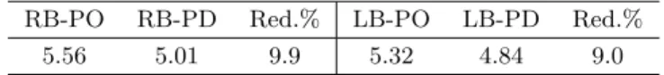
Results indicate that for both TI methods, using position and Doppler velocity measurements together provide an additional reduction in FTIP by an overall average factor of 27 to 199 depending on the maximum acceleration level while providing an acceptable level of TTIP as shown in Table 1. It should be noted that some of this reduction (approximately a factor of 5) in FTIP is due to the proposed usage of the sign information of the Doppler velocity measurements. Another apparent outcome is that increasing the minimum velocity threshold towards the approximated maximum Doppler velocity of the undesired measurements results in the even more reduction in FTIP. However, it also reduces the TTIP so that the minimum TTIP requirement cannot be met. Using the calculated FTIPs for both methods with the parameters given above, a performance comparison between the investigated TI schemes have also been made in terms of FTIP. The comparison has revealed that FTIP for the logic-based scheme is less than FTIP for the rule-based scheme probably due to its adjustable gate radius parameter. Computational complexity of the TI schemes given as average CPU time per scan is also investigated in case of the existence of only false measurements with PF A = 10−4, M = 3. The simulation results in Table 2 show that using 3D position and Doppler velocity measurements for TI has a moderate improvement on the CPU time. When Doppler velocity measurements are utilized along with position measurements while initiating a track, many false measurements get discarded, due to the added gatings employed based on Doppler measurements, which renders the processing time smaller than that of the position only case. In Table 2, the performance of the logic-based TI method is also superior to its competitor with respect to the CPU time.
Table 2. Average CPU time (sec.) comparison of the TI methods (RB: rule-based TI, LB: logic-based TI, PO: position only measurements, PD: position and Doppler velocity measurements, Red.%: percentage of reduction in CPU time).
RB-PO RB-PD Red.% LB-PO LB-PD Red.%
10-1 8 10-1 7 10-1 6 10-1 5 10-1 4 10-1 3 10-1 2 10-1 1 10-1 0 10-9 0.78 0.79 0.8 0.81 0.82 0.83 0.84 0.85 0.86 0.87
False Track Initiation Probability, P
FTI
True Track Initiation Probability, P
TTI
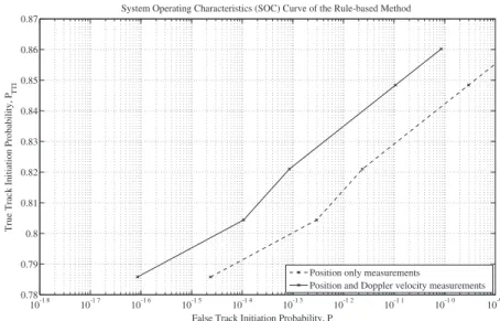
System Operating Characteristics (SOC) Curve of the Rule-based Method
Position only measurements
Position and Doppler velocity measurements
Figure 6. System Operating Characteristics of the rule-based TI scheme for both position only and position plus Doppler velocity measurements.
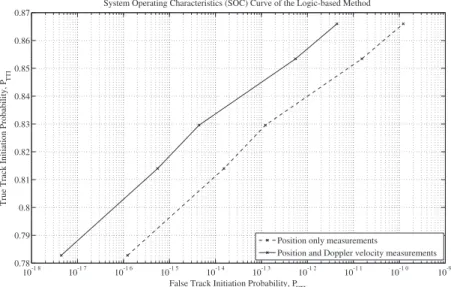
When FTIP is utilized instead of the false alarm probability in the conventional signal detection, the SOC curve is used instead of ROC curve. Similar to the ROC curve, SOC curve also provides a functional utility for performance observation of the TI unit in terms of FTIP and through SOC; TTIP and FTIP are interrelated. Although the SOC curve can be obtained for all the benchmark targets, for the sake of clarity, in this paper it is illustrated only for a randomly chosen benchmark target, e.g., target 3. Fig. 6 and Fig. 7 present the SOC curves for the rule- and logic-based TI methods for position only and position plus Doppler velocity measurement cases respectively (amax = 70 m/s2). An important outcome that is revealed both in Fig. 6 and Fig. 7 is that, for the both TI schemes, the extra information provided by the Doppler measurements decreases the probability of incorrectly initiating a track for the same TTIP. Looking at the issue from the other hand, at the same FTIP, an increased TTIP is obtained when both position and Doppler velocity measurements are available concurrently.
10-1 8 10-1 7 10-1 6 10-1 5 10-1 4 10-1 3 10-1 2 10-1 1 10-1 0 10-9 0.78 0.79 0.8 0.81 0.82 0.83 0.84 0.85 0.86 0.87
False Track Initiation Probability, P
FTI
True Track Initiation Probability, P
TTI
System Operating Characteristics (SOC) Curve of the Logic-based Method
Position only measurements
Position and Doppler velocity measurements
Figure 7. System Operating Characteristics of the logic-based TI scheme for both position only and position plus Doppler velocity measurements.
4. CONCLUSIONS
Analytical evaluation of FTIP for the most commonly used sequential TI schemes, the rule-based and logic-based schemes have been expanded to include elevation and Doppler velocity measurements. The advantage of using the Doppler velocity measurements in TI has been demonstrated both analytically and through simulations. Using position and Doppler velocity measurements together provide an additional reduction in FTIP by the average factor of 27 to 199 depending on the maximum acceleration. It should be noted that some of this reduction (approximately a factor of 5) is due to the usage of the sign information of the Doppler velocity measurements. However, due to the additional tests for the Doppler velocity case, average percentage of reduction of TTIP is approximately 6% which still satisfies the preset TTIP requirement. When the Doppler velocity measurements are used, the computational complexity and in effect track initiation time are also decreased by an average of 9.5%. Moreover, the derived closed form expressions for the FTIP provide a very useful tool for performance evaluation of the TI schemes avoiding time consuming simulations.
APPENDIX A. DERIVATION OF P3
Here, the derivation of p3 in (4) for 3D position measurements extracted by the PAR is given. Detailed expressions can be found in [22]. Let di,i+1 be distance between two measurements at the ith and (i + 1)th sampling times. It is calculated as:
di,i+1 =p(xi− xi+1)2+ (yi− yi+1)2+ (zi− zi+1)2 (A1) Consider that a target has a constant acceleration between short enough successive sampling times, di,i+1 is:
di,i+1 = υi,i+1ts+ 0.5ai+1t2s (A2) where υi,i+1is the estimated velocity obtained by using a measurement pair satisfying (1) and (2) at the ith and (i + 1)th sampling times; ai+1 = (υi,i+1− υi−1,i) t−1s is the estimated acceleration. Using (A2) for i = 1, 2 yields in
d2,3− d1,2= (υ2,3− υ1,2)ts+ 0.5(a3− a2)t2s (A3) If constant acceleration is considered, then
a3= a2 (A4)
υ2,3= υ1,2+ a2ts (A5)
are gained. Substituting (A4) and (A5) into (A3) results in
|d2,3− d1,2| = |a2|t2s≤ Ra (A6) where, unlike given in [10]‡, R
a = a∆ maxt2s, then using (1) and (A6), the following constraint is obtained for velocity and acceleration requirements as:
(R1≤ d2,3≤ R2) ∩ (|d2,3− d1,2| ≤ Ra) (A7) Rewriting the second half of the above constraint,
−Ra≤ d2,3− d1,2 ⇔ d2,3≥ d1,2− Ra
d2,3− d1,2≤ Ra ⇔ d2,3≤ d1,2+ Ra (A8) are obtained. Reorganizing (A8) and the first half of (A7) gives
R3 ≤ d2,3≤ R4 (A9)
If the first half of (A7) and boundaries of d2,3 in (A8) are combined, R3 and R4 are found as [10]:
R3= max(R1, d1,2− Ra)
R4 = min(R2, d1,2+ Ra) (A10) ‡ in [10], Rais erroneously given as Ra∆= 0.5amaxt2
At the 3rd sampling time, probability of having more than one undesired measurement obeying the constraints given by (A7) can be calculated similarly with (3) taken as:
PF,3= 1 − exp(−[[(NbζPF A)p3) (A11) In the above equation, probability p3, a measurement at the 3rd sampling time, conforms with the constraint of (A9) given the existence of a measurement pair obeying the velocity gating in (1) at the 1st and 2nd sampling times is defined as:
p3= P (R∆ 3 ≤ d2,3 ≤ R4 |R1 ≤ d1,2 ≤ R2) (A12) To calculate this conditional probability, if certain definitions are made as D1 = R∆ 1 + Ra, D2 = R∆ 2 − Ra, then R1 ≤ D1 ≤ D2 ≤ R2 is obtained [10]. Furthermore using (A10),
R3= ½ R1 R1≤ d1,2≤ D1 d1,2−Ra D1≤ d1,2≤ R2 R4= ½ d1,2+Ra R1≤ d1,2≤ D2 R2 D2≤ d1,2≤ R2 (A13) are obtained [10]. Now, the purpose is to calculate p3 using the partial expressions given by (A13). Taking into account the intervals [R1, D1] , (D1, D2], (D2, R2] given by (A13), p3 can be written as the sum of its parts as [10]:
p3= P (R3 ≤ d2,3 ≤ R4 |R1 ≤ d1,2 ≤ R2) = p3,1+ p3,2+ p3,3 (A14) In (A14), p3,1= P (R∆ 1≤ d2,3≤ d1,2+ Ra, R1≤ d1,2≤ D1|R1≤ d1,2≤ R2) (A15) p3,2= P (d∆ 1,2−Ra≤ d2,3≤ d1,2+Ra, D1≤ d1,2≤ D2|R1≤ d1,2≤ R2)(A16) p3,3= P (d∆ 1,2− Ra≤ d2,3≤ R2, D2≤ d1,2≤ R2|R1≤ d1,2≤ R2) (A17) and they need to be calculated. Following discussion is about the calculation of (A15), (A16) and (A17).
Since spatial density of the undesired measurements is uniform, probability that a position measurement falls into the region [R1, R2] can be written as [1]:
f ((x2, y2, z2) |R1 ≤ d1,2≤ R2|) = ½ 1
V2 R1 ≤ d1,2 ≤ R2
0 otherwise (A18)
Probability of any measurement given as a random variable (x2, y2, z2) falling into the volume V2 is [27]:
P (x2, y2, z2 ∈ V2) = Z Z Z
V2
where f (x2, y2, z2) is the joint probability density function. Using (A18) and (A19),
p3,1= 1 V2 Z Z Z R1≤d1,2≤D1 V3 Vs dx2dy2dz2 (A20) In (A20), V3is the volume of velocity and acceleration gate and is given as: V3 = 4 3π(R 3 4− R33) (A21)
Substituting (A13) and (A21) into (A20) gives p3,1 = 3V4π sV2 Z Z Z R1≤d1,2≤D1 ¡ (d1,2+ Ra)3− R31 ¢ dx2dy2dz2 (A22) Using Jacobian transformation rule [27], an integral calculation given in Cartesian coordinates is transformed into a new integral with the spherical coordinates as [27]: Z Z Z R f (x2, y2, z2)dx2dy2dz2 = Z Z Z V f (r, θ, φ)r2|− cos φ| drdθdφ (A23) In (A23), dV = dx2dy2dz2 = r2|− cos φ| drdθdφ stands for the unit volume element of a single beam of the PAR. Using the given transformation and coverage angles of the PAR for TI, namely in azimuth from θ1 to θ2 and in elevation from φ1 to φ2 where θ1 < θ2 and φ1< φ2 < π/2, it is obtained p3,1= 4π 3VsV2 Z Z Z R1≤d1,2≤D1 ³ (d1,2+ Ra)3− R13 ´ dx2dy2dz2 = 4π 3VsV2 φ2 Z φ1 θ2 Z θ1 D1 Z R1 ³ (r + Ra)3− R31 ´ r2cos φdrdθdφ =4π (θ2− θ1) (sin φ2− sin φ1) 3VsV2 D1 Z R1 r2 ³ (r + Ra)3− R13 ´ dr =4π (θ2− θ1) (sin φ2− sin φ1) 3VsV2 µ 1 6(R1+ Ra) 6 −1 6R 6 1 + 3 5Ra ³ (R1+ Ra)5− R51 ´ +3 4R 2 a ³ (R1+ Ra)4− R41 ´ + 1 3 ³¡ R3a− R31¢(R1+ Ra)3− R31 ´¶ (A24)
Similarly, p3,2=3V4π sV2 Z Z Z D1≤d1,2≤D2 ³ (d1,2+ Ra)3− (d1,2− Ra)3 ´ dx2dy2dz2 = 4π 3VsV2 φ2 Z φ1 θ2 Z θ1 D2 Z D1 ³ (r + Ra)3− (r − Ra)3 ´ r2cos φdrdθdφ =4π (θ2− θ1) (sin φ2− sin φ1) 3VsV2 D2 Z D1 r2 ³ (r + Ra)3− (r − Ra)3 ´ dr =4π (θ2− θ1) (sin φ2− sin φ1) 3VsV2 µ 6 5Ra(R2− Ra) 5 − (R1+ Ra)5 +2 3R 3 a(R2− Ra)3− (R1+ Ra)3 ¶ (A25) Finally, p3,3 is calculated as:
p3,3= 4π 3VsV2 Z Z Z D2≤d1,2≤R2 ³ R32− (d1,2− Ra)3 ´ dx2dy2dz2 = 4π 3VsV2 φ2 Z φ1 θ2 Z θ1 R2 Z D2 ³ R32− (r − Ra)3 ´ r2cos φdrdθdφ =4π (θ2− θ1) (sin φ2− sin φ1) 3VsV2 R2 Z D1 r2 ³ R32− (r − Ra)3 ´ dr =4π (θ2− θ1) (sin φ2− sin φ1) 3VsV2 µ −1 6 R 6 2 + 1 6(R2− Ra) 6+3 5Ra ³ R52− (R2− Ra)5 ´ −3 4R 2 a ³ R42− (R2− Ra)4 ´ +1 3 ¡ R32+ R3a¢ ³R32− (R2− Ra)3 ´ (A26) Substituting (A22)–(A26) into (A14), p3 can be found, and using it in (A11), PF,3 is calculated.
REFERENCES
1. Bar-Shalom, Y., Multitarget-Multisensor Tracking: Principles and Techniques, YBS, 1995.
2. Blackman, D. and R. Popoli, Design and Analysis of Modern Tracking Systems, Artech House, 1999.
3. Shi, Z. G., S. H. Hong, and K. S. Chen, “Tracking airborne targets hidden in blind doppler using current statistical model particle filter,” Progress In Electromagnetics Research, PIER 82, 227–240, 2008.
4. Zhang, W., Z. G. Shi, S. Du, and K. S. Chen, “Novel roughening method for reentry vehicle tracking using particle filter,” Journal of Electromagnetic Waves and Applications, Vol. 21, No. 14, 1969– 1981, 2007.
5. Bi, S. Z. and X. Y. Ren, “Maneuvering target doppler-bearing tracking with signal time delay using interacting multiple model algorithms,” Progress In Electromagnetics Research, PIER 87, 15– 41, 2008.
6. Turkmen, I. and K. Guney, “Tabu search tracker with adaptive neuro-fuzzy inference system for multiple target tracking,” Progress In Electromagnetics Research, PIER 65, 169–185, 2006. 7. Haridim, M., H. Matzner, Y. Ben-Ezra, and J. Gavan,
“Cooperative targets detection and tracking range maximization using multimode ladar/radar and transponders,” Progress In Electromagnetics Research, PIER 44, 217–229, 2004.
8. Chen, J. F., Z. G. Shi, S. H. Hong, and K. S. Chen, “Grey prediction based particle filter for maneuvering target tracking,” Progress In Electromagnetics Research, PIER 93, 237–254, 2009. 9. Leung, H., Z. Hu, and M. Blanchette, “Evaluation of multiple
target track initiation techniques in real radar tracking environ-ments,” IEE Proceedings of Radar, Sonar, Navigation, Vol. 143, No. 4, 246–253, 1996.
10. Hu, Z., H. Leung, and M. Blanchette, “Effectiveness of the likelihood function in logic based track formation,” IEEE Transactions on Signal Processing, Vol. 45, No. 2, 445–456, 1997. 11. Xue, W. and X. W. Sun, “Multiple targets detection method based on binary hough transform and adaptive time-frequency filtering,” Progress In Electromagnetics Research, PIER 74, 309–317, 2007. 12. Park, S. H., K. K. Park, J. H. Jung, K. T. Kim, and H. T. Kim,
“ISAR imaging of multiple targets using edge detection and hough transform,” Journal of Electromagnetic Waves and Applications, Vol. 22, No. 2/3, 365–373, 2008.
13. Bar-Shalom, Y., K. C. Chang, and H. M. Shertukde, “Performance evaluation of cascaded logic for track formation in clutter,” IEEE Transactions on Aerospace and Electronic Systems, Vol. 25, No. 6,
873–877, 1989.
14. Bar-Shalom, Y. and X. Li, “Effectiveness of the likelihood function in logic based track formation,” IEEE Transactions on Aerospace and Electronic Systems, Vol. 27, No. 1, 184–187, 1991.
15. Chang, K., S. Mori, and C. Chong, “Performance evaluation of track initiation in dense target environment,” IEEE Transactions on Aerospace and Electronic Systems, Vol. 30, No. 1, 213–219, 1994.
16. Cassassolles, E., M. Ludovic, S. Herve, and B. Tomasini, “Integration of radar measurement attributes in the multiple hypothesis tracker results for track initiation,” Proceedings of SPIE, Signal and Data Processing of Small Targets, Vol. 2759, 397–403, 1996.
17. Lacle, L. and J. Driessen, “Velocity-based track discrimination algorithms,” IEE Target Tracking: Algorithms and Applications, Vol. 2759, 4.1–4.4, 1996.
18. Fitzgerald, R., “Simple tracking filters: Position and velocity measurements,” IEEE Transactions on Aerospace and Electronic Systems, Vol. 18, 531–537, 1982.
19. Farina, A. and S. Pardini, “Track-while scan algorithm in a clutter environment,” IEEE Transactions on Aerospace and Electronic Systems, Vol. 14, 769–778, 1978.
20. Kural, F. and Y. Ozkazanc, “A method for detecting RGPO/VGPO jamming,” IEEE Signal Processing and Commu-nications Applications Conference, 237–240, 2004.
21. Kural, F., F. Arıkan, O. Arıkan, and M. Efe, “Incorporating doppler velocity measurement for track initiation and mainte-nance,” IEE Seminar on Target Tracking: Algorithms and Ap-plications, 107–114, 2006.
22. Kural, F., “Performance improvement of the multiple target tracking algorithms with the incorporation of doppler velocity measurement,” PhD thesis, Hacettepe University, 2006.
23. Wang, X., D. Musicki, and R. Ellem, “Fast track confirmation for multi-target tracking with doppler measurements,” 3rd International Conference on Intelligent Sensors, Sensor Networks and Information, ISSNIP, 263–268, 2007.
24. Wang, X., D. Musicki, R. Ellem, and F. Fletcher, “Enhanced multi-target tracking with doppler measurements,” Information, Decision and Control, IDC, 53–58, 2007.
25. Blair, W., G. Watson, T. Kirubarajan, and Y. Bar-Shalom, “IMMPDAF for radar management and tracking benchmark with
ECM,” IEEE Transactions on Aerospace and Electronic Systems, Vol. 44, No. 4, 1115–1134, 1998.
26. Kirubarajan, T., Y. Bar-Shalom, and E. Daeipour, “Adaptive beam pointing control of a phased array radar in the presence of ECM and false alarms using IMMPDAF,” Proceedings of American Control Conference, 2616–2620, 1995.
27. Papoulis, A., Probability, Random Variables, and Stochastic Processes, 3rd edition, McGraw-Hill International Editions, 1991. 28. Barton, D., Modern Radar System Analysis, Artech House, 1988. 29. Hatamzadeh-Varmazyar, S., “Calculating the radar cross section of the resistive targets using the haar wavelets,” Progress In Electromagnetics Research, PIER 83, 55–80, 2008.
30. Wang, Y. B. and Y. M. Bo, “Fast RCS computation with general asymptotic waveform evaluation,” Journal of Electromagnetic Waves and Applications, Vol. 21, No. 13, 1873–1884, 2007. 31. Carpentieri, B., “Fast large RCS calculation using the boundary
element method,” Journal of Electromagnetic Waves and Applications, Vol. 21, No. 14, 1959–1968, 2007.
32. Wang, S. G., X. P. Guan, D. W. Wang, X. Y. Ma, and Y. Su, “Fast calculation of wide-band responses of complex radar targets,” Progress In Electromagnetics Research, PIER 68, 185–196, 2007. 33. Blair, W. D., G. A. Watson, S. Hoffman, and G. L. Gentry,
“Benchmark problem for beam pointing control of phased array radar against maneuvering targets in the presence of ECM and false alarms,” Proceedings of American Control Conference, 2601– 2605, Seattle WA, 1995.