Projecting the flow variables for hub location problems

Projecting the Flow Variables for Hub Location Problems

Martine Labbe´

Universite´ Libre de Bruxelles, De´partement d’Informatique, Boulevard du Triomphe CP 210/01, 1050 Bruxelles, Belgium

Hande Yaman

Bilkent University, Department of Industrial Engineering, 06800 Bilkent, Ankara, Turkey

We consider two formulations for the uncapacitated hub location problem with single assignment (UHL), which use multicommodity flow variables. We project out the flow variables and determine some extreme rays of the projection cones. Then we investigate whether the cor-responding inequalities define facets of the UHL polyhe-dron. We also present two families of facet defining inequalities that dominate some projection inequalities. Finally, we derive a family of valid inequalities that gen-eralizes the facet defining inequalities and that can be separated in polynomial time.© 2004 Wiley Periodicals, Inc. NETWORKS, Vol. 44(2), 84 –93 2004

Keywords: hub location; projection; dicut inequalities; polyhe-dral analysis

1. INTRODUCTION

In this article, we consider the Uncapacitated Hub Lo-cation Problem with Single Assignment (UHL). Let I denote the set of terminal nodes with 兩I兩 ⫽ n and K the set of commodities. For commodity k 僆 K, o(k) is the origin, d(k) is the destination and tkis the amount of traffic where tk ⫽ to(k)d(k). Origins and destinations of commodities are

terminal nodes, and any distinct pair of terminal nodes defines a commodity.

Each terminal either receives a hub or is connected to another node that receives a hub. If node i僆 I is connected to such a node j僆 I⶿{i}, then the traffic on the link between nodes i and j is the traffic adjacent at node i, that is, the total traffic of commodities with node i as origin or destination. The cost of routing this traffic on the link between node i and node j is denoted by Fij. Any node i that becomes a hub

is assigned to itself. The cost of installing a hub at node i is denoted by Fii.

Let A ⫽ {( j, l ) : j 僆 I, l 僆 I, j ⫽ l} and Rjl denote

the cost of routing a traffic unit on arc ( j, l ) if it becomes a backbone arc, that is, if both nodes j and l receive hubs. We assume that the cost vector R satisfies the triangle inequality and Rjl ⱖ 0 for all ( j, l ) 僆 A. In addition, we

assume that all data are rational.

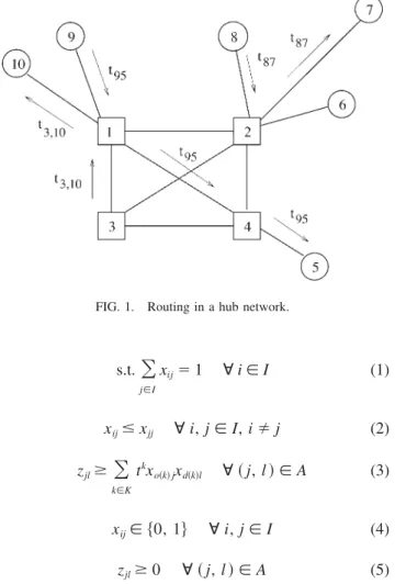
If two nodes i and m are assigned to the same hub, say j, the traffic from node i to node m follows the path i 3 j3 m. However, if node i is assigned to node j and node m is assigned to node l, then the traffic from node i to node m follows the path i 3 j 3 l 3 m. Therefore, the total traffic on arc ( j, l ) is the sum of the traffic of commodities whose origins are assigned to node j and whose destinations are assigned to node l. In Figure 1, we see a network with 10 nodes where nodes 1, 2, 3, and 4 are hub nodes. The traffic from node 9 to node 5 follows the path 93 1 3 4 3 5, because node 9 is assigned to node 1 and node 5 is assigned to node 4. The traffic from node 8 to node 7 goes through the path 8 3 2 3 7, as both nodes 8 and 7 are assigned to node 2. Finally, the traffic from node 3 to node 10 goes from node 3 to node 1 and then to node 10, because node 3 is a hub and so is assigned to itself and node 10 is assigned to node 1.

The aim of UHL is to choose the hub locations and assign the terminal nodes to hubs to minimize the total cost of location and routing. It has applications in transportation and telecommunication. The UHL is an NP-hard problem (see Yaman [10] for the proof for the special case where Rjl

⫽ 0 for all ( j, l ) 僆 A). For a recent survey on applications and solution methods, see Campbell et al. [3].

Let xijbe 1 if node i僆 I is assigned to node j 僆 I and

0 otherwise. If node i receives a hub then xiiis 1 and node

i is assigned to itself. Further, define zjlto be the total traffic

on the arc ( j, l )僆 A. We can formulate UHL as follows:

min

冘

i僆Ij

冘

僆I

Fijxij⫹

冘

共 j,l 兲僆A

Rjlzjl

Received June 2003; accepted January 2004

Correspondence to: H. Yaman; e-mail: hyaman@bilkent.edu.tr

Contract grant sponsor: France Telecom R&D; contract grant number: 99 1B 774

DOI 10.1002/net.20019

Published online in Wiley InterScience (www.interscience. wiley.com).

s.t.

冘

j僆I xij⫽ 1 ᭙ i 僆 I (1) xijⱕ xjj ᭙ i, j 僆 I, i ⫽ j (2) zjlⱖ

冘

k僆K tk xo共k兲 jxd共k兲l ᭙ 共 j, l 兲 僆 A (3) xij僆 兵0, 1其 ᭙ i, j 僆 I (4) zjlⱖ 0 ᭙ 共 j, l 兲 僆 A (5)

Constraints (1), (2), and (4) imply that each node either receives a hub or is assigned to exactly one other node which receives a hub. For (i, j) 僆 A such that Rjl ⬎ 0,

constraints (3) compute the value of traffic in terms of the assignment variables.

In this article, we present two ways of linearizing con-straints (3). These linearizations use the flow variables Xjl k

⫽ xo(k) jxd(k)lfor k僆 K and j 僆 I, l 僆 I and they have the

same linear programming bound (see Yaman [10]). The number of flow variables is O(n4). So these linearizations are huge in size and not very useful in practice. We discuss how to project out these flow variables to obtain a formu-lation of a smaller size. Then we investigate the domination among the projection inequalities. Finally, we prove that some of these inequalities are facet defining for the hub location polyhedron. We also introduce two other families of facet-defining inequalities that dominate some of the projection inequalities. Then we give a family of valid inequalities which generalizes the facet defining inequali-ties.

This article is organized as follows: In Section 2, we present the multicommodity formulation. We project out the flow variables in two different ways and compare the pro-jection inequalities. In Section 3, we project out the flow variables in the hub location formulation and characterize the extreme rays of the projection cone for a single

com-modity. Then we present some families of extreme rays for the multicommodity case. In Section 4, we summarize the previous polyhedral results for the UHL and present new facet-defining inequalities.

2. MULTICOMMODITY FLOW LINEARIZATION AND ITS PROJECTIONS

As the routing cost R satisfies the triangle inequality, we can formulate UHL using multicommodity flows. To obtain the multicommodity flow formulation, we replace con-straints (3) with the following set of inequalities:

冘

l僆I⶿兵 j其 Xlj k ⫺

冘

l僆I⶿兵 j其 Xjl k ⱕ xd共k兲 j⫺ xo共k兲 j ᭙ j 僆 I, k 僆 K (6)

冘

k僆K tk Xjl k_{ⱕ z} jl ᭙ 共 j, l 兲 僆 A (7) Xjl k_{ⱖ 0 ᭙ 共 j, l 兲 僆 A, k 僆 K} (8) Notice that the flow balance equations are replaced by the equivalent inequality forms (6) (see Mirchandani [6]). These constraints state that if the origin of commodity k is assigned to hub j but not the destination, there is a net flow of one unit that goes out of hub j. On the contrary, if the destination is assigned to j but not the origin, there is a net flow of one unit that comes into node j. If both the origin and destination are assigned to j or neither one is assigned to j, the flow on the arcs incoming to node j is equal to the flow on the arcs outgoing from node j concerning this commodity. As the routing cost satisfies the triangle in-equality, these constraints guarantee that the traffic of a commodity uses the direct link between the hubs of its origin and destination if its origin and destination are as-signed to different hubs.

Constraints (7) imply that the traffic on arc ( j, l ) should be at least the sum of the traffic of commodities whose origins are assigned to node j and whose destinations are assigned to node l. We sometimes refer to the traffic on the backbone links as capacity to be able to follow the termi-nology of flows and cuts.

To our knowledge, there are two ways of projecting out the flow variables in this system. The first method used by Mirchandani [6] is a direct projection. This method leads to inequalities known as the metric inequalities (see Iri [4] and Onaga and Kakusho [7]). Mirchandani [6] studies the ex-treme rays of the resulting cone for the single commodity and multicommodity cases. For the single commodity case the projection inequalities are the well-known cut inequal-ities. However, for the multicommodity case, we do not know any characterization of all the extreme rays of the resulting cone.

The second method used by Rardin and Wolsey [8] is to replace the flow constraints by the corresponding cut

straints and do the projection afterwards. The projection inequalities are called dicut inequalities.

Here, we do the projection using both methods and compare the results. The comparison gives us a necessary condition for the dicut inequalities not to be dominated. 2.1. Projection 1: Direct Method

First, we follow the method used by Mirchandani [6]. If we associate dual variables␣_jk _{to constraints (6) and␤}

jlto

constraints (7), by Farkas’ Lemma, we have the following result: given a solution x and z, there exists a vector X satisfying (6)–(8) if and only if

冘

共 j,l 兲僆A zjl␤jlⱖ

冘

k僆K

冘

j僆I tk_{共 x} o共k兲 j⫺ xd共k兲 j兲␣j k (9)

for all (␣, ␤) ⱖ 0 such that ␤jlⱖ␣j

k_⫺␣ l

k _{᭙ k 僆 K, 共 j, l 兲 僆 A}

(10) For a 僆 ⺢, let (a)⫹ ⫽ max{0, a}. As zjlⱖ 0 for all ( j,

l )僆 A and all the data are rational, for a given ( x, z) there exists a vector X that satisfies (6)–(8) if and only if

冘

共 j,l 兲僆A zjlmax k僆K共␣j k_⫺␣ l k_兲⫹_ⱖ

冘

k僆Kj

冘

僆I tk_共x o共k兲 j⫺ xd共k兲 j兲␣j k (11)

for all integer␣j k _{ⱖ 0.}

2.2. Projection 2: Indirect Method

We now do the projection as in Rardin and Wolsey [8]. Let uak denote the capacity of arc a used for commodity k.

For x, which satisfies (1), (2), and (4), there exists a feasible flow for commodity k if and only if

冘

a僆␦共S兲 ua k ⱖ tk

冘

j僆S 共 xo共k兲 j⫺ xd共k兲 j兲 ᭙ S 債 I

where␦(S) ⫽ {( j, l ) 僆 A : j 僆 S, l 僆 I⶿S} is the cut induced by cut set S. So the inequalities (6)–(8) can be replaced by the following:

冘

a僆␦共S兲 ua k_{ⱖ t}k

冘

j僆S 共 xo共k兲 j⫺ xd共k兲 j兲 ᭙ S 債 I, k 僆 K (12)

冘

k僆K ua k ⫽ za ᭙ a 僆 A (13) ua k_{ⱖ 0 ᭙ a 僆 A, k 僆 K} (14) If we associate dual variables␥S

k _{ⱖ 0 to inequalities (12)}

and␴a to equations (13) we get that, given ( x, z) which

satisfies (1), (2), (4), and (5) there exists a vector X satis-fying (6)–(8) if and only if

冘

a僆A za␴aⱖ

冘

S債Ik

冘

僆K tk

冘

j僆S 共 xo共k兲 j⫺ xd共k兲 j兲␥S k (15)

for all (␥, ␴) such that ␴aⱖ

冘

S:a僆␦共S兲 ␥S k _{᭙ k 僆 K, a 僆 A} ␥S k_{ⱖ 0 ᭙ k 僆 K, S 債 I}

This condition is equivalent to

冘

a僆A zamax k僆K 兵

冘

S:a僆␦共S兲 ␥S k_{其 ⱖ}

冘

S債Ik

冘

僆K tk

冘

j僆S 共xo共k兲 j⫺ xd共k兲 j兲␥S k (16)

for all integer␥ ⱖ 0 as all data are rational and zaⱖ 0 for

all a 僆 A. The ␥S

k

s are interpreted in Rardin and Wolsey [8] as follows: if we let ⌫k denote a collection of cut sets for commodity k, we can interpret␥S

k

as the number of times cut set S is repeated in the collection⌫k.

2.3. Comparison of Projections 1 and 2

Proposition 1. For a given␥, define ⌫kto be the collec-tion of cut sets for k僆 K, that is, S is repeated␥S

k

times in ⌫k

. Then for a given (x, z) which satisfies (1), (2), (4), and (5), there exists a vector X that satisfies (6)–(8) if and only if (16) is satisfied for all integer␥ ⱖ 0 such that we can rename the cut sets in ⌫k as S1

k , . . . , Snk⫺1 k , Snk k where nk

⫽ 兩⌫k_{兩 in such a way that S} nk k _{債 S} nk⫺1 k _{債 . . . 債 S} 1 k for all k 僆 K.

Proof. Consider inequality (15) for (␥, ␴) ⱖ 0 such that␥ is integer and ␴a⫽ maxk僆K{¥S債I:a僆␦(S) ␥S

k } for all a僆 A. Define␣j k _{⫽ ¥} S債I:j僆S ␥S k . Then ␣j k is the number of times node j is repeated in the cut sets in collection⌫k. The right hand side of inequality (15) is equal to

冘

S債Ik

冘

僆Kj

冘

僆S tk_{共 x} o共k兲 j⫺ xd共k兲 j兲␥S k ⫽

冘

k僆K

冘

j僆I S債I:j僆S

冘

tk_{共 x} o共k兲 j⫺ xd共k兲 j兲␥S k ⫽

冘

k僆K

冘

j僆I tk_{共 x} o共k兲 j⫺ xd共k兲 j兲␣j k

which is equal to the right-hand side of inequality (9) for this␣.

Now we compare the left hand sides. For ( j, l )僆 A and k 僆 K, 共␣j k ⫺␣l k 兲⫹_{⫽ 共}

冘

S債I:j僆S ␥S k ⫺

冘

S債I:l僆S ␥S k 兲⫹ ⱕ 共

冘

S債I:j僆S ␥S k ⫺

冘

S僆⌫k_{:l僆S, j僆S} ␥S k 兲⫹_⫽

冘

S債I:共 j,l 兲僆␦共S兲 ␥S k

Let k⬘ be such that maxk僆K(␣j k _{⫺ ␣} l k )⫹ ⫽ (␣j k⬘_{⫺ ␣} l k⬘ )⫹. It follows that ␴jl⫽ max k僆K兵S債I:共 j,l 兲僆␦共S兲

冘

␥S k_{其 ⱖ}

冘

S債I:共 j,l 兲僆␦共S兲 ␥S k⬘ ⱖ max k僆K 共␣j k_⫺␣ l k_兲⫹_⫽␤ jl

Hence, the left-hand side of inequality (15) is greater than or equal to the left-hand side of inequality (9). As the right-hand sides are equal, inequality (9) dominates inequality (15).

Next, we show how we can construct a pair (␥, ␴) that gives the same inequality as a given (␣, ␤) pair. For each commodity k, let ␣k _{⫽ max}

j僆I␣jk. Define ⌫k to be the

collection of sets Sik for i⫽ 1, 2, . . . , ␣k where Sik⫽ { j

僆 I :␣jkⱖ i} so that we have S␣k k

債 S␣k_⫺1 k

債 . . . 債 S1k for

all k僆 K. Define also␥S_ik k

to be the number of times Si k

is repeated in⌫kfor all i ⫽ 1, 2, . . . ,␣kand k 僆 K. For S ⰻ ⌫k , set ␥S k _{⫽ 0. Then␣} j k _{⫽ ¥} S債I:j僆S ␥S k . Moreover, if ␣j k_{⬎ ␣} l k

, then whenever l僆 S, we have j 僆 S. Therefore, ␣j k_⫺␣ l k_⫽

冘

S債I:j僆S ␥S k_⫺

冘

S債I:l僆S ␥S k ⫽

冘

S債I:j僆S ␥S k ⫺

冘

S僆⌫k_{:l僆S, j僆S} ␥S k ⫽

冘

S債I:共 j,l 兲僆␦共S兲 ␥S k and if␣_jk _{ⱕ ␣} l k_{, then there is no S} i k _{債 I such that ( j, l )} 僆 ␦(Si k_{). So}

冘

S債I:共 j,l 兲僆␦共S兲 ␥S k_{⫽ 0 ⫽ 共␣} j k_⫺␣ l k_兲⫹

This proves that 共␣j k_⫺␣ l k_兲⫹_⫽

冘

S債I:共 j,l 兲僆␦共S兲 ␥S k

for all ( j, l ) 僆 A and k 僆 K.

Hence, for inequalities (16), it is enough to consider⌫ where we can sort the cut sets in each⌫k such that Snk

k _債

Snkk⫺1債 . . . 債 S1

k

where nkis the number of cut sets in⌫ k

.

■

This result implies that the inequalities (16) that do not satisfy the condition of Proposition 1 are dominated by

inequalities (11). So in a solution procedure based on cuts, one does not need to separate these dominated inequalities. 3. HUB LOCATION LINEARIZATION AND ITS PROJECTION

To obtain the hub location linearization, we replace constraints (3) by

冘

l僆I Xjl k ⱖ xo共k兲 j ᭙ j 僆 I, k 僆 K (17) ⫺

冘

j僆I Xjl k_{ⱖ ⫺x} d共k兲l ᭙ l 僆 I, k 僆 K (18) ⫺

冘

k僆K tk Xjl k_{ⱖ ⫺z} jl ᭙ 共j, l兲 僆 A (19) Xjl k_{ⱖ 0 ᭙ 共 j, l 兲 僆 A, k 僆 K} (20) This formulation is given in Skorin-Kapov et al. [9]. Note that we replaced constraints (17) and (18), which are orig-inally equalities by their equivalent inequality forms. This formulation is different from the multicommodity formula-tion given in the previous secformula-tion as it explicitly imposes that every commodity travels from the hub of its origin to the hub of its destination directly. If the origin and destina-tion of a commodity k are assigned to the same hub, say j, then the variable Xjj

k

takes value 1 (these variables did not exist in the multicommodity formulation).

Proposition 2. Given (x, z), there exists X that satisfies (17)–(20) if and only if

冘

a僆A za␤aⱖ

冘

k僆K tk

冘

j僆I 共 xo共k兲 j␣j k_{⫺ x} d共k兲 j␴j k_兲 (21)

for all (␣, ␴, ␤) ⱖ 0 such that ␤jlⱖ␣j k_⫺␴ l k _{᭙ k 僆 K, 共 j, l 兲 僆 A} (22) 0ⱖ␣j k ⫺␴j k ᭙ k 僆 K, j 僆 I (23) Proof. If we associate dual variables␣jkto constraints

(17),␴lk to constraints (18) and␤jl to constraints (19), by

Farkas’ Lemma, we get the result. ■

Notice that inequalities (11) form a subset of the projec-tion inequalities of this hub locaprojec-tion linearizaprojec-tion. More precisely, inequalities (11) correspond to inequalities (21) for integer (␣, ␴, ␤) ⱖ 0 which satisfy ␣j

k _{⫽ ␴} j k

for all k 僆 K and j 僆 I and␤jl⫽ maxk僆K(␣j

k_{⫺ ␴} l k

) for all ( j, l ) 僆 A. However, remaining inequalities (21) are not neces-sarily dominated by inequalities (11). This is natural as the routing of the hub location is also feasible for the multi-commodity formulation.

Let H be the cone of (␣, ␴, ␤) ⱖ 0 that satisfy inequal-ities (22) and (23). Nondominated projection inequalinequal-ities are among inequalities (21) that are defined by (␣, ␴, ␤), which are extreme rays of H (see Balas [2]).

We consider first the case for a single commodity and characterize all nondominated inequalities. This gives us insight for the multicommodity case.

3.1. Single Commodity Case

Suppose兩K兩 ⫽ 1. We drop the index k from the variables defined above.

Proposition 3. The ray (␣, ␴, ␤) ⫽ (0, 0, 0) is extreme for cone H if and only if it belongs to one of the classes:

1. ␤jl ⫽ 1 for some ( j, l ) 僆 A and the other entries

are zero.

2. ␴j ⫽ 1 for some j 僆 I and the other entries are

zero.

3. ␣j⫽ 1 for all j 僆 S, where S 債 I, ␴l⫽ 1 for all l

僆 I and the other entries are zero.

4. ␣j ⫽ 1 for all j 僆 S where S 債 I, ␴l ⫽ 1 for all l

僆 T where T 債 I such that S 債 T,␤jl⫽ 1 if j 僆 S,

l ⰻ T and the other entries are zero.

Proof. The proof is very similar to the proof of Prop-osition 3.5 given by Mirchandani [6]. We give it here for the sake of completeness.

(Sufficiency) Classes 1 and 2 are trivial. For classes 3 and 4, consider (␣, ␴, ␤) ⫽ (0, 0, 0) 僆 H. Let B ⫽ {( j, l )僆 A :␤jl⬎ 0}, S ⫽ { j 僆 I :␣j⬎ 0} and T ⫽ {l 僆 I

:␴l⬎ 0}. Notice that S 債 T because of the constraint (23).

Suppose that (␣, ␴, ␤) is not an extreme ray of H. Then there exist distinct (␣, ␴, ␤)1and (␣, ␴, ␤)2in H, which are not multiples of (␣, ␴, ␤) and (␣, ␴, ␤) ⫽ 1/2(␣, ␴, ␤)1 ⫹ 1/2(␣, ␴, ␤)2

. This implies that␣j

1 _{⫽ ␣} j 2_{⫽ 0 if j ⰻ S,} ␴j 1 _{⫽ ␴} j 2 _{⫽ 0 if j ⰻ T and␤} jl 1 _{⫽ ␤} jl 2 _{⫽ 0 if ( j, l ) ⰻ B.} In Class 3, B⫽ A and T ⫽ I. As␤jl 1 _{⫽ ␤} jl 2 _{⫽ 0 for all} ( j, l ) in A,␴l 1_{ⱖ ␣} j 1 and␴l 2_ⱖ␣ j 2

for all j僆 S and l 僆 I. As␣j 1_⫹␣ j 2_{⫽ 2␣} j⫽ 2 and␴l 1_{⫹ ␴} l 2_{⫽ 2␴} l⫽ 2 we have that␴l 1_{⫽ ␣} j 1_{⫽ ␥}1 and␴l 2 _{⫽ ␣} j 2_{⫽ ␥}2

for all j 僆 S and l僆 I. Then (␣, ␴, ␤)1and (␣, ␴, ␤)2are multiples of (␣, ␴, ␤).

In Class 4, B, S, and T are all nonempty. If j僆 S and l 僆 T, then␤jl⫽ 0. So we have␴l 1_{ⱖ ␣} j 1 and␴l 2_ⱖ␣ j 2 for all j僆 S and l 僆 T. By the above discussion,␴l

1_{⫽ ␣} j 1_⫽ ␥1 and␴l 2 _{⫽ ␣} j 2 _{⫽ ␥}2

for all j 僆 S and l 僆 T. If j僆 S and l ⰻ T, then␤jl 1 _{ⱖ ␣} j 1 and␤jl 2 _ⱖ␣ j 2 . As␣j 1 ⫹ ␣j 2 _{⫽ 2␣} j ⫽ 2 and␤jl 1 _{⫹ ␤} jl 2 _{⫽ 2␤} jl ⫽ 2, we get␤jl 1 ⫽ ␣j 1_{⫽ ␥}1 and␤jl 2 _{⫽ ␣} j 2 _{⫽ ␥}2 . So (␣, ␴, ␤)1and (␣, ␴, ␤)2 are multiples of (␣, ␴, ␤).

For classes 3 and 4, we showed that a ray (␣, ␴, ␤) satisfying the requirements of one of these classes cannot be written as a linear combination of two distinct rays of H. Thus, such a ray (␣, ␴, ␤) is an extreme ray.

(Necessity) Given an extreme ray (␣, ␴, ␤) ⫽ (0, 0, 0) of

H, define the sets B, S, and T. Assume that S⫽ A. It is easy to show that if T⫽ A, then (␣, ␴, ␤) should belong to class 1 and if B⫽ A then (␣, ␴, ␤) should belong to class 2. If both T and B are not empty, then this can be written as a linear combination of rays of classes 1 and 2, so it cannot be extreme.

Now, assume that S⫽ A. By feasibility, we have S 債 T. Define␥ ⫽ min{minj僆S␣j, minl僆T␴l}. Clearly,␥ ⬎ 0.

Consider the two rays (␣, ␴, ␤)1and (␣, ␴, ␤)2defined as follows:␣j 1_{⫽ ␥ for all j 僆 S, ␴} l 1_{⫽ ␥ for all l 僆 T, ␤} jl 1 ⫽␥ for all j 僆 S, l ⰻ T, ␣j 2_{⫽ 2␣} j⫺ ␥ for all j 僆 S, ␴l 2 ⫽ 2␴l ⫺ ␥ for all l 僆 T, ␤jl 2 _{⫽ 2␤} jl ⫺ ␥ for all j 僆 S, l ⰻ T, ␤jl 2 _{⫽ 2␤}

jl for all j 僆 S, l 僆 T or j ⰻ S and the

rest of entries are 0. Both (␣, ␴, ␤)1and (␣, ␴, ␤)2are in H and (␣, ␴, ␤) ⫽ 1/2(␣, ␴, ␤)1⫹ 1/2(␣, ␴, ␤)2. But as (␣, ␴, ␤) is an extreme ray, (␣, ␴, ␤)1

and (␣, ␴, ␤)2 should be multiples of (␣, ␴, ␤). So ␣j⫽ 1 for all j 僆 S, ␴l ⫽ 1 for

all l僆 T,␤jl ⫽ 1 for all j 僆 S, l ⰻ T and the rest of the

entries are 0.

If B⫽ A, by feasibility we have T ⫽ I. Then (␣, ␴, ␤) is in Class 3. Otherwise, it is in Class 4. ■

Proposition 4. Given (x, z) which satisfies (1), (2), (4), and (5), there exists X that satisfies (17)–(20) if and only if

冘

共 j,l 兲僆A:j僆S,lⰻT zjlⱖ t共

冘

j僆S xoj⫺

冘

l僆T xdl兲 (24) for all S債 T 債 I.

Proof. Inequalities (21) defined by (␣, ␴, ␤) that are extreme rays of H are as follows:

1. zjl ⱖ 0 for all ( j, l ) 僆 A.

2. xdjⱖ 0 for all j 僆 I.

3. ¥j僆Sxojⱕ 1 for all S 債 I.

4. ¥_{( j,l )僆A:j僆S,lⰻT}zjlⱖ t(¥j僆Sxoj⫺ ¥l僆Txdl) for all S

債 T 債 I.

The first three families of inequalities are implied by con-straints (5), (4), and (1), respectively. The only nonredun-dant inequalities are the inequalities of the fourth form. ■

These inequalities are quite similar to cut inequalities for the single commodity flow. In fact, when we take a cut in the case of hub location, we choose two disjoint subsets of the set I, S and T៮⫽ I⶿T and consider all the arcs going from S to T៮.

Proposition 5. Given (x, z), we can separate inequalities (24) by solving a min cut problem.

Proof. Separation of (24) is to find S 債 T 債 I such that ¥( j,l )僆A:j僆S,lⰻT zjl ⫺ t(¥j僆S xoj ⫺ ¥l僆T xdl) is

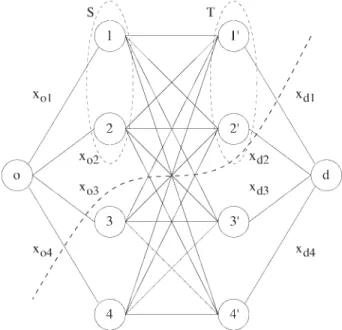
minimized. Let␾ denote this minimum value. Consider the layered graph G⬘ ⫽ (V, A⬘) where V includes the nodes o and d, the set I and a duplicate I⬘ of set I, that is, V ⫽ {o,

d} 艛 I 艛 I⬘. The arc set is A⬘ ⫽ {(o, j) : j 僆 I} 艛 {( j, l ) : j僆 I, l 僆 I⬘} 艛 {(l, d) : l 僆 I⬘}. Let w_ijdenote the capacity of arc (i, j)僆 A⬘ defined as follows:

woj⫽ txoj ᭙ j 僆 I

wld⫽ txdl ᭙ l 僆 I⬘

wjl⫽ zjl ᭙ j 僆 I, l 僆 I⬘ : 共 j, l 兲 僆 A

wjj⬘⫽ ⬁ ᭙ j 僆 I, j⬘ 僆 I⬘

A cut set C is a subset of the set V such that o僆 C and d ⰻ C. Define S ⫽ C 艚 I and T ⫽ C 艚 I⬘. If the duplicates of nodes in S are not in T, the cut has an infinite capacity. Otherwise, the capacity of cut set C is

冘

共i, j兲僆␦共C兲 wij⫽

冘

jⰻS txoj⫹

冘

j僆S

冘

lⰻT zjl⫹

冘

l僆T txdl ⫽ t ⫺

冘

j僆S txoj⫹

冘

l僆T txdl⫹

冘

j僆S

冘

lⰻT zjl

As cut set C⫽ {o} has capacity t, the min cut problem has a finite value. So,␾ ⫽ minC ¥(i, j)僆␦(C) wij ⫺ t. ■

In Figure 2, the set C⫽ {o, 1, 2, 1⬘, 2⬘}. So S ⫽ {1, 2}, T ⫽ {1⬘, 2⬘} and the corresponding inequality is:

z13⫹ z14⫹ z23⫹ z24ⱖ t共 xo1⫹ xo2⫺ xd1⫺ xd2兲

3.2. Multicommodity Case

Now we consider the multicommodity case. For (␣, ␴, ␤) ⫽ (0, 0, 0) in H, define B ⫽ {( j, l ) 僆 A :␤jl ⬎ 0}, Sk ⫽ { j 僆 J : ␣j k_{⬎ 0} and T} k ⫽ {l 僆 I : ␴l k _{⬎ 0} for all} k 僆 K and K⬘ ⫽ {k 僆 K : Sk ⫽ A}.

The extreme rays for which B ⫽ A or K⬘ ⫽ A are characterized as follows:

1. If Sk ⫽ Tk ⫽ A for all k 僆 K, then (␣, ␴, ␤) is an

extreme ray if and only if␤jl⫽ 1 for some ( j, l ) 僆 A

and the rest of entries are zero. The corresponding pro-jection inequality is zjl ⱖ 0.

2. If Sk⫽ A for all k 僆 K and B ⫽ A, then (␣, ␴, ␤) is

an extreme ray if and only if␴j k

⫽ 1 for some j 僆 I and for some k 僆 K and the rest of the entries are 0. The corresponding projection inequality is x_{d(k) j}ⱖ 0. 3. If B⫽ A and Sk債 I for all k 僆 K⬘, then we should have

Tk ⫽ I for all k 僆 K⬘. In this case, (␣, ␴, ␤) is an

extreme ray if and only if兩K⬘兩 ⫽ 1. The corresponding projection inequality is ¥j僆Skxo(k) jⱕ 1.

These propositions can be proved in a similar way to the proof of Proposition 3.

We have a sufficient condition for a special class of the remaining rays to be extreme.

Proposition 6. (Labbe´ et al. [5]) Let Sk債 Tk債 I for all k

僆 K. Define (␣, ␴, ␤) such that ␣j k_{⫽ 1 j 僆 S} k ␴l k_{⫽ 1 l 僆 T} k

␤jl⫽ 1 if there exists a k 僆 K such that j 僆 Skand lⰻTk

and the other entries are 0. Then (␣, ␴, ␤) 僆 H.

Define G⬘ ⫽ (B, E) where B ⫽ {(j, l) 僆 A :␤jl⫽ 1} and

E⫽ {{(j, l), (m, n)} : (j, l) 僆 B, (m, n) 僆 B,␤jl⫽␣j k

and ␤mn⫽ ␣m

k

for some k 僆 K}. For k 僆 K, define also the bipartite graph G⬘k⫽ (Sk⫻ Tk, E⬘k) where E⬘k⫽ {{j, l} : j

僆 Sk, l僆 Tk,␤jl⫽ 0 or j ⫽ l}.

Ray (␣, ␴, ␤) is extreme if graphs G⬘ and G⬘k are

connected for all k僆 K and Sk⫽ I for all k 僆 K.

A special class of these extreme rays define inequalities that are similar to inequalities (24).

Proposition 7. (Labbe´ et al. [5]) The inequality

冘

j僆S l

冘

僆T zjlⱖ

冘

k僆K⬘ tk_关

冘

j僆S xo共k兲 j⫹

冘

l僆T xd共k兲l⫺ 1兴 (25)

where S and T are nonempty disjoint subsets of I and K⬘ 債 K is a valid inequality, and it is not dominated by other projection inequalities.

Moreover, a subset of these inequalities are indeed sufficient to have a formulation of UHL.

Proposition 8. (Labbe´ et al. [5]) For (x, z) which satisfies (1), (2), (4), and (5), there exists X that satisfies (17)–(20) if and only if (x, z) satisfies inequalities

zjlⱖ

冘

k僆K⬘

tk_{共 x}

o共k兲 j⫹ xd共k兲l⫺ 1兲 ᭙ K⬘ 債 K, 共 j, l 兲 僆 A

(26) For the single commodity case, these inequalities sim-plify to

zjlⱖ t共 xoj⫹ xdl⫺ 1兲 ᭙ 共 j, l 兲 僆 A

zjlⱖ 0 ᭙ 共 j, l 兲 僆 A

This corresponds to the classical way of linearizing con-straints zjl ⫽ txojxdl for all ( j, l )僆 A when we minimize

a cost function where variables zjls have positive

coeffi-cients.

4. FACETS OF THE UHL POLYHEDRON

Polyhedral properties of UHL are studied in Labbe´ et al. [5]. Here we summarize their results and present some new facet defining inequalities.

We replace constraints (3) by (26) to have a linear formulation. We also eliminate the variables xjjs by

substi-tuting xjj⫽ 1 ⫺ ¥m僆I⶿{ j}xjmfor all j僆 I (see Avella and

Sassano [1]).

If both j and l become hubs, then the traffic of commod-ities with destination j or origin l does not travel on arc ( j, l ). Moreover, the traffic from node j to node l travels on arc ( j, l ). Define Kjl⫽ K⶿({( j, l )} 艛 {(m, j) : m 僆 I⶿{ j}}

艛 {(l, m) : m 僆 I⶿{l}}).

The UHL can be reformulated as follows: min

冘

i僆Ij僆I⶿兵i其

冘

Fijxij⫹

冘

i僆I Fii共1 ⫺

冘

j僆I⶿兵i其 xij兲 ⫹

冘

共 j,l 兲僆A Rjlzjl s.t. xij⫹

冘

m僆I⶿兵 j其 xjmⱕ 1 ᭙ 共i, j兲 僆 A (27) zjlⱖ

冘

k僆K⬘:o共k兲⫽j,d共k兲⫽e tk 共 xo共k兲 j⫹ xd共k兲l⫺ 1兲 ⫹

冘

i僆I⶿兵 j,l其:共 j,i兲僆K⬘ tji共 xil⫺

冘

m僆I⶿兵 j其 xjm兲 ⫹

冘

i僆I⶿兵 j,l其:共i,l 兲僆K⬘ til共 xij ⫺

冘

m僆I⶿兵l其 xlm兲 ⫹ tjl共1 ⫺

冘

m僆I⶿兵 j其 xjm⫺

冘

m僆I⶿兵l其 xlm兲 ᭙ K⬘ 債 Kjl,共 j, l 兲 僆 A (28) xij僆 兵0, 1其 ᭙ 共i, j兲 僆 A (29) zjlⱖ 0 ᭙ 共 j, l 兲 僆 A (30) Let PUH⫽ conv({( x, z) 僆 {0, 1} n(n⫺1)_{⫻ ⺢}n(n⫺1)_{: ( x,} z) satisfies (27)–(30)}). Define eij x _{⫽ ( x, z) (resp. e} ij z _{⫽ ( x,}

z)) to be the unit vector such that xlm ⫽ 0 for all (l, m)

僆 A⶿{(i, j)}, xij⫽ 1 and zlm⫽ 0 for all (l, m) 僆 A (resp.

xlm⫽ 0 for all (l, m) 僆 A, zlm⫽ 0 for all (l, m) 僆 A⶿{(i,

j)} and zij ⫽ 1).

Proposition 9. (Labbe´ et al. [5]) The polyhedron PUH is

full dimensional, that is, dim(PUH)⫽ 2n(n ⫺ 1).

Theorem 1. (Labbe´ et al. [5]) The inequality ␲x ⱕ ␲0

defines a facet of PUHif and only if it defines a facet of PUC

⫽ conv{x 僆 {0, 1}n(n⫺1) _{: x}

ij ⫹ ¥m僆I⶿{j} xjm ⱕ 1 @(i, j)

僆 A}.

The polytope PUC is a special stable set polytope. For

facet defining inequalities of PUC, see Yaman [10]. Theorem 2. (Labbe´ et al. [5]) No inequality of the form␤z ⱖ␤0defines a facet of PUHunless it is a positive multiple

of zjlⱖ 0 for some (j, l) 僆 A.

Proposition 10. (Labbe´ et al. [5]) For (j, l)僆 A, if tjl⫽ 0,

then the inequality zjl ⱖ 0 defines a facet of PUH.

The remaining facet defining inequalities of PUHinvolve

both x and z variables. Here, we investigate which inequal-ities (28) are facet defining inequalinequal-ities.

Proposition 11. For (j, l) 僆 A and K⬘ 債 Kjl, define I⬘j

⫽ {m 僆 I⶿{l} : ?i 僆 I⶿{m} : (i, m) 僆 K⬘, tim⬎ 0} and I⬘l

⫽ {m 僆 I⶿{j} : ?i 僆 I⶿{m} : (m, i) 僆 K⬘, tmi ⬎ 0}. If

inequality (28) defines a facet of PUH, then I⬘j ⫽ I⬘l⫽ A. Proof. Assume that ( x, z) 僆 PUH satisfies inequality

(28) at equality and that xjm⫽ 1 for some m 僆 I⬘j. Then the

right-hand side of inequality (28) is

冘

k僆K⬘:o共k兲⫽j,d共k兲⫽e tk_{共 x} d共k兲l⫺ 1兲 ⫹

冘

i僆I⶿兵 j,l其:共 j,i兲僆K⬘ tji共 xil⫺ 1兲 ⫺

冘

i僆I⶿兵 j,l其:共i,l 兲僆K⬘ til

冘

m僆I⶿兵l其 xlm⫺ tjl

冘

m僆I⶿兵l其 xlm ⱕ

冘

k僆K⬘:o共k兲⫽j,d共k兲⫽e tk_{共 x} d共k兲l⫺ 1兲 ⫹

冘

i僆I⶿兵 j,l其:共 j,i兲僆K⬘ tji共 xil⫺ 1兲 ⱕ

冘

i僆I⶿兵m其:共i,m兲僆K⬘ tim共 xml⫺ 1兲 ⫽ ⫺

冘

i僆I⶿兵m其:共i,m兲僆K⬘ tim⬍ 0

So, any ( x, z) 僆 PUH that satisfies inequality (28) at

equality also satisfies xjm⫽ 0 for m 僆 I⬘j. We can show that

( x, z) should also satisfy xlm ⫽ 0 for m 僆 I⬘lin a similar

way. So if at least one of sets I⬘j and I⬘l is nonempty, then

inequality (28) is not facet defining for PUH. ■

If tk ⫽ 0 for all k 僆 K⬘, then both sets I⬘j and I⬘l are

empty. We next show that in this case, inequality (28) is facet defining. Define N to be a very large integer.

Proposition 12. For (j, l)僆 A, if tk⫽ 0 for all k 僆 K⬘, then inequality (28) is facet defining for PUH.

Proof. Assume that tk ⫽ 0 for all k 僆 K⬘. Below are 2n(n⫺ 1) affinely independent points in PUH that satisfy

inequality (28) at equality: ● ¥_{(t,s)僆A⶿{( j,l )}} Nets z ⫹ tjlejl z ● ¥_{(t,s)僆A⶿{( j,l )}}Nets z _{⫹ t} jlejl z _{⫹ e} im

z _{for (i, m) 僆 A⶿{( j,}

l )} ● eim x _{⫹ ¥} (t,s)僆A⶿{( j,l )}Nets z _{⫹ t} jlejl

z _{for i僆 I⶿{ j, l} and}

m 僆 I⶿{i, j, l} ● ejm x _{⫹ ¥} (t,s)僆A⶿{( j,l )} Nets z _{for m 僆 I⶿{ j}} ● elm x ⫹ ¥(t,s)僆A⶿{( j,l )} Nets z for m 僆 I⶿{l} ● eij x _{⫹ e} lj x _{⫹ ¥} (t,s)僆A⶿{( j,l )} Nets z _{for i僆 I⶿{ j, l}} ● eil x ⫹ ejl x ⫹ ¥(t,s)僆A⶿{( j,l )} Nets z for i僆 I⶿{ j, l}. ■

In the sequel, we present two more families of facet-defining inequalities that dominate some projection inequal-ities.

Proposition 13. For (j, l)僆 A, the inequality zjlⱖ tjl共1 ⫺

冘

i僆I⶿兵 j其 xji⫺

冘

i僆I⶿兵l其 xli兲 ⫹

冘

i僆I⶿兵 j,l其 tji共 xil⫺

冘

m僆I⶿兵i, j其 xjm兲 ⫹

冘

i僆I⶿兵 j,l其 til共 xij⫺

冘

m僆I⶿兵i,l其 xlm兲 (31) is valid for PUH.

Proof. If xji ⫽ xli ⫽ 0 for all i 僆 I⶿{ j, l}, then

inequality (31) is the same as inequality (28) for K⬘ ⫽ {( j, i) : i僆 I⶿{ j, l}} 艛 {(i, l ) : i 僆 I⶿{ j, l}}. If xjp⫽ 1 for

some p 僆 I⶿{ j, l}, then the right-hand side of inequality (31) is ⫺tjl

冘

i僆I⶿兵l其 xli⫹

冘

i僆I⶿兵 j,l,p其 tji共xil⫺ 1兲 ⫺

冘

i僆I⶿兵 j,l其 til

冘

m僆I⶿兵i,l其 xlmⱕ 0

The case where xlp⫽ 1 for some p 僆 I⶿{ j, l} is analogous.

■

The proof of Proposition 13 shows that inequality (31) dominates inequality (28) for K⬘ ⫽ {( j, i) : i 僆 I⶿{ j, l}} 艛 {(i, l ) : i 僆 I⶿{ j, l}}.

Proposition 14. For (j, l)僆 A, inequality (31) defines a facet of PUH.

Proof. Below are 2n(n ⫺ 1) affinely independent points in PUHthat satisfy inequality (31) at equality:

● ¥_{(t,s)僆A⶿{( j,l )}} Nets z ⫹ tjlejl z ● ¥_{(t,s)僆A⶿{( j,l )}}Nets z _{⫹ t} jlejl z _{⫹ e} im z

for (i, m) 僆 A⶿{( j, l )} ● eim x _{⫹ ¥} (t,s)僆A⶿{( j,l )}Nets z _{⫹ t} jlejl z

for i僆 I⶿{ j, l} and m 僆 I⶿{i, j, l} ● ejm x _{⫹ ¥} i僆I⶿{ j,l,m} eil x _{⫹ ¥} (t,s)僆A⶿{( j,l )} Nets z for m 僆 I⶿{ j} ● elm x _{⫹ ¥} i僆I⶿{ j,l,m} eij x _{⫹ ¥} (t,s)僆A⶿{( j,l )} Nets z for m 僆 I⶿{l} ● eij x _{⫹ ¥} (t,s)僆A⶿{( j,l )} Nets z _{⫹ (t} jl ⫹ til)ejl z for i 僆 I⶿{ j, l} ● eil x _{⫹ ¥} (t,s)僆A⶿{( j,l )} Nets z _{⫹ (t} jl ⫹ tji)ejl z for i 僆 I⶿{ j, l}. ■

Proposition 15. For (j, l)僆 A, Ij債 I⶿{j, l} and Il債 I⶿{j,

l} such that Ij艚 Il⫽ A and Ij艛 Il⫽ I⶿{j, l}, the inequality

zjlⱖ

冘

i僆Ijm

冘

僆Il tim共 xij⫹ xml⫹ xim⫹ xmi⫺ 1兲 ⫹

冘

i僆Il tji共 xil⫺

冘

m僆I⶿兵i, j其 xjm兲 ⫹

冘

i僆Ij til共 xij⫺

冘

m僆I⶿兵i,l其 xlm兲 ⫹ tjl共1 ⫺

冘

i僆I⶿兵 j其 xji⫺

冘

i僆I⶿兵l其 xli兲 (32) is valid for PUH.

Proof. Assume that xim ⫽ xmi⫽ 0 for all i 僆 Ij and

m 僆 Il and xjm ⫽ xlm ⫽ 0 for all m 僆 I⶿{ j, l}. Then

inequality (32) is the same as inequality (28) for K⬘ ⫽ {(i, m)僆 K : i 僆 Ij, m僆 Il}艛 {(i, l ) 僆 K : i 僆 Ij} 艛 {( j,

i) 僆 K : i 僆 Il} and is valid. If xjm ⫽ 1 for some m

僆 I⶿{ j} then we can show that inequality (32) is still valid as in the proof of Proposition 13. So inequality (32) is valid if xim⫽ xmi⫽ 0 for all i 僆 Ij and m 僆 Il. Notice that if

xim⫹ xmi⫽ 1 for some i 僆 Ij and m僆 Ilthen xij ⫹ xml

⫽ 0. So inequality (32) is valid for PUH. ■

Inequality (32) dominates inequality (28) for K⬘ ⫽ {(i, m)僆 K : i 僆 Ij, m僆 Il}艛 {(i, l ) 僆 K : i 僆 Ij} 艛 {( j,

i) 僆 K : i 僆 Il}.

Proposition 16. For (j, l)僆 A, Ij債 I⶿{j, l} and Il債 I⶿{j,

l} such that Ij艚 Il⫽ A and Ij艛 Il⫽ I⶿{j, l}, inequality (32)

defines a facet of PUH.

Proof. Below are 2n(n ⫺ 1) affinely independent points in PUHthat satisfy inequality (32) at equality:

● ¥p僆Ijepj x ⫹ ¥(t,s)僆A⶿{( j,l )} Nets z ⫹ ¥p僆Ij艛{ j}tplejl z ● ¥p僆Ij eij x _{⫹ ¥} (t,s)僆A⶿{( j,l )} Nets z _{⫹ ¥} p僆Ij艛{ j} tplejl z _⫹ eim z

for (i, m) 僆 A⶿{( j, l )}

● eim x _{⫹ ¥} p僆Il⶿{m} epl x _{⫹ ¥} p僆Ij⶿{i} epj x _{⫹ ¥} (t,s)僆A⶿{( j,l )} Nets z

⫹ ¥p僆Ij⶿{i}艛{ j}¥r僆Il⶿{m}艛{l}tprejl

z for i僆 Ijand m 僆 Il ● emi x ⫹ ¥p僆Il⶿{m} epl x ⫹ ¥p僆Ij⶿{i} epj x ⫹ ¥(t,s)僆A⶿{( j,l )} Nets z _{⫹ ¥}

p僆Ij⶿{i}艛{ j}¥r僆Il⶿{m}艛{l}tprejl

z for i僆 Ijand m 僆 Il ● eim x _{⫹ ¥} p僆Il epl x _{⫹ ¥} (t,s)僆A⶿{( j,l )} Nets z _{⫹ ¥} p僆Il艛{l} tjpejl z for i 僆 Ijand m 僆 Ij ● eim x _{⫹ ¥} p僆Ij epj x _{⫹ ¥} (t,s)僆A⶿{( j,l )} Nets z _{⫹ ¥} p僆Ij艛{ j} tplejl z for i 僆 Iland m 僆 Il ● eij x _{⫹ ¥} p僆Ilepl x _{⫹ ¥} (t,s)僆A⶿{( j,l )}Nets z _{⫹ ¥} p僆Il艛{l}(tip ⫹ tjp)ejl z for i 僆 Ij

● eil x _{⫹ ¥} p僆Ilepl x _{⫹ e} jl x _{⫹ ¥} (t,s)僆A⶿{( j,l )}Nets z for i僆 Ij ● eil x ⫹ ¥p僆Ijepj x ⫹ ¥(t,s)僆A⶿{( j,l )}Nets z ⫹ ¥p僆Ij艛{ j}(tpi ⫹ tpl)ejl z for i 僆 Il ● eij x ⫹ ¥p僆Ijepj x ⫹ elj x ⫹ ¥(t,s)僆A⶿{( j,l )}Nets z for i僆 Il ● eji x _{⫹ ¥} p僆Ilepl x _{⫹ ¥} (t,s)僆A⶿{( j,l )}Nets z for i僆 Ij艛 {l} ● eji x ⫹ ¥p僆Il⶿{i} epl x ⫹ ¥p僆Ij epi x ⫹ ¥(t,s)僆A⶿{( j,l )}Nets z for i 僆 Il ● eli x ⫹ ¥p僆Ijepj x ⫹ ¥(t,s)僆A⶿{( j,l )}Nets z for i僆 Il艛 { j} ● eli x _{⫹ ¥} p僆Ij⶿{i} epj x _{⫹ ¥} p僆Il epi x _{⫹ ¥} (t,s)僆A⶿{( j,l )}Nets z for i 僆 Ij. ■

Before concluding this section, we discuss the separation problems related to inequalities (28), (31), (32), and (33). For ( j, l ) 僆 A, inequalities (28) can be separated in polynomial time by taking

K⬘ ⫽ 兵共i, m兲 僆 Kjl: i, m僆 I⶿兵 j, l其, xo共k兲 j⫹ xd共k兲l ⬎ 1其 艛 兵i 僆 I⶿兵 j, l其 : xil⬎

冘

m僆I⶿兵 j其 xjm其 艛 兵i 僆 I⶿兵 j, l其 : xij ⬎

冘

m僆I⶿兵l其 xlm其

Inequalities (31) can also be separated in polynomial time by enumeration. However, the separation of inequali-ties (32) seems more complicated. In fact, this separation problem is a special max cut problem on a graph Gc⫽ (I,

Ac). Let wadenote the capacity of arc a僆 Ac. The arcs and

their capacities are defined as follows: 共 j, i兲 : i 僆 I⶿兵 j, l其 wji⫽ tji共 xil⫺

冘

m僆I⶿兵i, j其 xjm兲 共i, l 兲 : i 僆 I⶿兵 j, l其 wil⫽ til共 xij⫺

冘

m僆I⶿兵i,l其 xlm兲 共i, m兲 : i, m 僆 I⶿兵 j, l其 wim⫽ tim共 xij⫹ xml⫹ xim⫹ xmi⫺ 1兲 共 j, l 兲 wjl⫽ tjl共1 ⫺

冘

i僆I⶿兵 j其 xji⫺

冘

i僆I⶿兵l其 xli兲

The capacity of a max cut separating j and l in Gc is

equal to the maximum value that the right-hand side of inequality (32) can attain. So for ( j, l ) 僆 A, the most violated inequality (32) can be found by solving a max cut problem.

We now present a family of valid inequalities that gen-eralizes inequalities (32) and that can be separated in poly-nomial time.

Proposition 17. For (j, l)僆 A and K⬘ 債 Kjl, the inequality

zjlⱖ

冘

k僆K⬘:o共k兲⫽j,d共k兲⫽e tk_{共 x} o共k兲 j⫹ xd共k兲l⫹ xo共k兲d共k兲⫹ xd共k兲o共k兲⫺ 1兲 ⫹

冘

i僆I⶿兵 j,l其:共 j,i兲僆K⬘ tji共 xil⫺

冘

m僆I⶿兵i, j其 xjm兲 ⫹

冘

i僆I⶿兵 j,l其:共i,l 兲僆K⬘ til共 xij ⫺

冘

m僆I⶿兵i,l其 xlm兲 ⫹ tjl共1 ⫺

冘

m僆I⶿兵 j其 xjm⫺

冘

m僆I⶿兵l其 xlm兲 (33) is valid for PUH.

Proof. Similar to the proof of Proposition 15. ■

Clearly, for a given ( j, l )僆 A and K⬘ 債 Kjl, inequality

(33) dominates inequality (28). Propositions 12 and 17 imply the following:

Corollary 1. For (j, l)僆 A and K⬘ 債 Kjl, inequality (28)

is facet defining for PUHif and only if t

k_{⫽ 0 for all k 僆 K⬘.}

Inequalities (33) can be separated in polynomial time by taking for ( j, l ) 僆 A,

K⬘ ⫽ 兵共i, m兲 僆 Kjl: i, m僆 I⶿兵 j, l其, xo共k兲 j⫹ xd共k兲l⫹ xo共k兲d共k兲

⫹ xd共k兲o共k兲⬎ 1其 艛 兵i 僆 I⶿兵 j, l其 : xil⬎

冘

m僆I⶿兵i, j其

xjm其

艛 兵i 僆 I⶿兵 j, l其 : xij⬎

冘

m僆I⶿兵i,l其

xlm其

In the example below, we show that using inequalities (33), we can cut some fractional solutions that do not violate inequalities (28).

Example 1. Assume that I⫽ {1, 2, 3, 4} and the only nonzero traffic demand is from node 3 to node 4 and t34⫽ 1.

Consider (x, z) such that x31 ⫽ x42 ⫽ x34 ⫽ 0.5, the

remaining entries of x are zero and z⫽ 0. The vector (x, z) satisfies all inequalities (28). Inequality (33) for arc (1, 2) and K⬘ ⫽ {(3, 4)} is

z12ⱖ t34共 x31⫹ x42⫹ x34⫹ x43⫺ 1兲 ⫽ 0.5

So by introducing this inequality in the current LP relax-ation, we can cut off the point (x, z). ■

This example suggests that inequalities (33) can be useful in a branch and cut framework.

5. CONCLUSION

We considered two formulations for the UHL that are based on flow variables. The first formulation is the multi-commodity formulation. We presented two ways of project-ing out the flow variables in this formulation. We deter-mined some dicut inequalities that are dominated comparing the two projections.

Then we projected out the flow variables in the hub location formulation. The inequalities obtained from the projection of the hub location formulation include the

ine-qualities obtained from projection applied to the multicom-modity formulation.

For the hub location formulation, we characterized the extreme rays of the projection cone for the single commod-ity case and pointed out its relation to cuts for flows. For the multicommodity case, we identified some of the extreme rays. The projection inequalities defined by a subfamily of these rays is sufficient to have a valid formulation of UHL. We showed that some of these inequalities are facet defining while some others are dominated by other facet-defining inequalities. We also presented a family of valid inequalities that generalizes these facet-defining inequalities and that can be separated in polynomial time.

Acknowledgments

The support of France Telecom R&D is gratefully ac-knowledged. The authors are grateful to two anonymous referees for their comments and suggestions.

REFERENCES

[1] P. Avella and A. Sassano, On the p-median polytope, Math Program 89 (2001), 395– 411.

[2] E. Balas, “Projection and lifting in combinatorial

optimiza-tion,” Computational combinatorial optimization, M. Ju¨nger and D. Naddef (Editors), Springer, Berlin, 2001, pp. 26 –56. [3] J.F. Campbell, A.T. Ernst, and M. Krishnamoorthy, “Hub location problems,” Facility location: Applications and the-ory, Z. Drezner and H.W. Hamacher (Editors), Springer, Berlin, 2002, pp. 373– 407.

[4] M. Iri, On an extension of the max-flow min-cut theorem to multicommodity flows, J Operat Res Soc Jpn 13 (1971), 129 –135.

[5] M. Labbe´, H. Yaman, and E. Gourdin, A branch and cut algorithm for hub location problems with single assignment, ISRO/OR Series Preprint 2003/05, Universite´ Libre de Bruxelles, 2003. Available at http://smg.ulb.ac.be/. [6] P. Mirchandani, Projections of the capacitated network

loading problem, Eur J Operat Res 122 (2000), 534 –560. [7] K. Onaga and O. Kakusho, On the feasibility conditions of

multicommodity flows in networks, IEEE Transact Circuit Theory 18 (1971), 425– 429.

[8] R.L. Rardin and L.A. Wolsey, Valid inequalities and pro-jecting the multicommodity extended formulation for unca-pacitated fixed charge network flow problems, Eur J Operat Res 71 (1993), 95–109.

[9] D. Skorin-Kapov, J. Skorin-Kapov, and M. O’Kelly, Tight linear programming relaxations of uncapacitated p-hub me-dian problem, Eur J Operat Res 94 (1996), 582–593. [10] H. Yaman, Concentrator location in telecommunication

net-works, Ph.D. Thesis, Universite´ Libre de Bruxelles, 2002. Available at http://smg.ulb.ac.be/.