Selçuk J. Appl. Math. Selçuk Journal of Vol. 10. No. 1. pp. 147-155, 2009 Applied Mathematics
A Simple Discrete Model for the Growth Tumor Andrés Barrea, Cristina Turner
Universidad Nacional de Córdoba CIEM-CONICET, Argentina e-mail: abarrea@ fam af.unc.edu.ar,turner@fam af.unc.edu.ar
Received: May 5, 2009
Abstract. In this work we propose a discrete model for the growth tumor. This model is based on the continuous model in [1] which uses the conventional ideas of nutrient diffusion and consumption by the cells. We assume that region is two-dimensional and we discretize by means of a grid × where sites are occupied by the different types of tumor cells (proliferating, quiescent and dead) and normal cells. The growth rules are stochastic and depend on the concentration of nutrient. A discussion of the results and applications of the model are presented.
Key words: Growth Tumor - Stochastic Model. 2000 Mathematics Subject Classification: 95B05 93A30. 1.Introduction
A variety of models for tumor growth have been developed in the last decades Some models are based on reaction-diffusion equations ([5], [6]).
Other models include hyperbolic equations, we refer to ([1], [2], [3], [7]). In [1] the authors have studied a particular model with three cells populations: proliferating cells, quiescent cells and dead cells.
This model includes densities , , and of proliferating, quiescent and dead (necrotic) cell respectively, and concentration of nutrients (generally oxigen). These densities satisfy a system of nonlinear first order hyperbolic equations in the tumor, with tumor surface as a free boundary.
The cells in different states are assumed to be mixed within the tumor, and to have the same size. They assumed that the tumor is uniformly packed with cells, so that:
+ + = ≡
Due to proliferation of cells and to removal of necrotic cells, there is a continuous movement of cells within the tumor and that the field velocity −→ satisfies the Darcy’s law. They treat the tumor tissue as a porous medium, that is:
−
→ = ∇ pressure
In this model they assume that:
· () is increasing in (rate of change from proliferating state to
quiescent state).
· () is decreasing in (rate of change from quiescent state to
prolif-erating state).
· () is decreasing in (quiescent cells become necrotic at a rate
()).
· () is decreasing in (the death rate by apoptosis).
· () is increasing in (the proliferation rate).
· () ()
· is a positive constant. (the rate of removal of dead cells).
The concentration satisfies the next difussion equation:
∇2 − = 0 in Ω () ( 0) = 0 on Ω ()
where Ω is the tumor region at time
The densities , and satifies the following system:
+ div ( ) = £ () − () − () ¤ + () + div () = () − £ () + () ¤ + div () = () + () −
If we add the last equations then we obtain an equation for the pressure : ∇2 = () −
Now, we set
= 0 = =
∇2 = 0 in Ω () = 1 on Ω () + div (∇) = [() − () − ()] + () in Ω () + div (∇) = () − [() − ()] in Ω () ∇2 = −+ [() + ] + in Ω () where () = (0) for =
The pressure on the surface of the tumor is equal to the surface tension, that is:
= on Ω () ( 0)
where is the mean curvature. The motion of the free boundary is given by the continuity equation
−
→ · −→ = or
−→ = on Ω ()
where −→ is the outward normal and is the velocity of the free boundary of
the free boundary in the outward normal direction. Given initial conditions Ω (0) ( 0) ( 0)
we would like to determine the family of domains Ω() and the functions ( ), ( ), ( ) and ( ) satisfying the last system. We note that tumors grown in vitro are typically of spherical shape, which makes the study of radially sym-metric solutions quite relevant. The radialy symsym-metric case of the the general model is given by the following equations system:
1 2 µ 2 ¶ = (0 0 () 0) (0 ) = 0 ( () ) = 1 ( 0) + = [() − () − ()] + () − [(() + ) + − ] (0 ≤ ≤ () 0) + = () − [() + ()] − [(() + ) + − ] (0 ≤ ≤ () 0)
1 2 ¡ 2¢ = [ () + ] + − (0 ) = 0 ( 0) () = ( () ) ( 0) with initial data
(0) ( 0) ( 0)
The last system is a free boundary problem and its numerical solution is harder. In [9] a numerical solution has been proposed for this system by means of a spectral method.
In this paper we propose a stochastic version of this system of equations which is very simple and it respect the qualitative properties of the original model. 2.The Mathematical Model
We consider the square lattice (typically = 2 3).At each site in the square
lattice there is a kind of cell.
The kinds are health (0), proliferating (1), quiescent (2) and dead (3) cells. We denote our stochastic process by , where is the time.
In this work the time will be consider discrete.( i.e. = 1 2 3 ). For a site in
() = means that in the site there is a cell of kind = 0
1 2 3 in the time .
Thus, each site has four possible states.
We consider the configuration for the concentration of the nutrient (generally oxigen).
Other possible nutrient can be considered [8]. For a site in
() is the concentration of nutrient in the time .
Assume that the model is in the configuration then the state at the given site changes according to the following probabilities depending on the concentration of the nutrient in the 2 + 1 nearest neighbors of the site (we include the site ).
We use the notation ∼ to indicate that the site is one of the 2 + 1 nearest neighbors of the site .
We consider the following notation for the change probabilities for to +1. · 01 for 0 → 1 state 0 go to state 1.
· 12 for 1 → 2 state 1 go to state 2.
· 03 for 0 → 3 state 0 go to state 3.
· 21 for 2 → 1 state 2 go to state 1.
· 23 for 2 → 3 state 2 go to state 3.
We assume that = ( O ()) where O () = P ∼ () and are a real an positive parameters.
3. Choosing the probabilities and updating the concentration
In this section we choose the probabilities with that the cells change, it depends on the nutrient around it. This is according to the biological hypothesis. We choose the probabilities for each site as following:
· 01() = tanh (01O ()) · 12() = tanh (12O ()) · 03() = 1 − tanh (03O ()) · 21() = 1 − tanh (21O ()) · 23() = 1 − tanh (23O ()) · 30() = 1 − tanh (30O ())
At each time, we do the following change: 1. We check the kind do cell at the site
2. We choose uniformly 0 ≤ ≤ 1 a random number.
3. According to and we change the kind of cell at site .
Then, we change by +1 and updating . 4. Updating the concentration
The concentration of nutrient is update according to diffusion equation: = − div ( ( ) ∇)
We note that there is not consumption of nutrients for the cells.
At each time, the diffusion matrix $A$ is building by means the following coef-ficients:
· 0: Diffusion coefficient for the health cells.
· 1: Diffusion coefficient for the proliferating cells.
· 2: Diffusion coefficient for the quiescent cells.
· 3: Diffusion coefficient for the dead cells.
That is, the coefficient = if the site is occupied by a cell of kind .
The solution of the partial differential equation is obtained by means of the classical difference finite method.
5. Results and Simulations
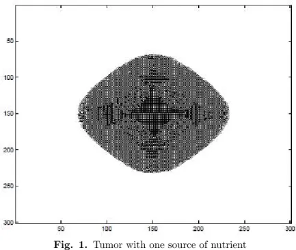
In these examples we show that the behavior of the simulation is the same as the solution of the original system, that is a central core of dead cells and the boundary of cells quiescent and proliferating is observed. The shape of the tumor is closer to the radial and the tumor growth around the source of nutrient. Example 1. In the examples, we consider the following values for the parame-ter:
01= 1 12= 10 03= 1 21= 001 23= 10 30= 5
0= 00025 1= 0001 2= 0003 3= 0004
The concentration of nutrient is considered with a constant source, equal to 1, in the middle of the tissue.
Fig. 1. Tumor with one source of nutrient
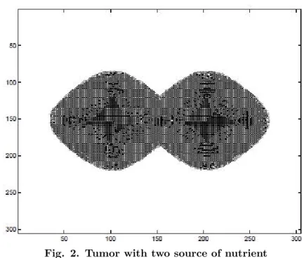
Example 2. In this example we consider the same values for the parameters but two source of nutrients are considered in this case. The dependence of the growth tumor of the nutrient source is clear at this simulation.
Fig. 2. Tumor with two source of nutrient
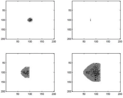
Example 3. First, we consider the resection of half tumor at = 40. We show the tumor for = 20 40 60 80. The tumor grows to recovering the radial symmetric shape around the nutrient source.
Now, we consider the resection of a lot of tumor at = 40. Again we show the tumor for = 20 40 60 80. The tumor grows to recovering the radial symmetric shape as the before example.
Fig. 4. Resection a lot of tumor 6. Conclusions
The model presented in this paper is a stochastic and simplified version of a sys-tem of differential equations with free boundary, which is of easy computational implementation.
The simulation satisfies the qualitative properties of the continuous model, that is a core of dead cells, the boundary of the quiescent and proliferating cells and the shape of tumor.
In the model presented in this paper, we consider a single nutrient and inho-mogeneties in the diffusivities. By solely varying the parameters (the diffusion coefficient) between reasonable bounds, we have different morphologies for the tumor. We observed the behavior of tumor according to the sources of nutrient and the resection. The impact of other treatments can also be modeled. References
1. S. Cui and A. Friedman (2003): A hyperbolic free boundary problem modeling tumor growth, Interfaces and Free Boundaries, 5, 159-181.
2. Cui S. and Friedman A. (2000): Analysis of a mathematical model of the effect of inhibitors on the growth of tumors, Math Biosci., 164, 103-137.
3. Cui S. and Friedman A. (2001): Analysis of a mathematical model of the growth of necrotic tumors, J. Math. Anal. Appl., 255, 636-677.
4. Adam J. (1986):A simplified mathematical model of tumor growth, Math. Biosci., 81, 224-229.
5. Byrne H. and Chaplain M.(1997): Free boundary value problems associated with growth and development of multicellular spheroids, European J. Appl. Math., 8, 639-658.
6. Pettet G., C. Please C., Tindall M. and McElwain D.(2001): The migration of cells in multicell tumor spheroids, Bull. Math. Biol., 63, 231-257.
7. Pescarmona G. P., Scalerandi M., Delsanto P. and Condat C. (1999): Non-linear model of cancer growth and metastasis: a limiting nutrient as a major determinant of tumor shape and diffusion, Medical Hypotheses, 53, 6, 497-503.
8. Barrea A. and Turner C. (2005): A numerical analysis of a model of a growth tumor, Applied Mathematics and Computation, 167, 345-354.