3871
Missing Events in Event Studies: Identifying the Effects
of Partially Measured News Surprises
†By Refet S. Gürkaynak, Burçin Kısacıkog˘lu, and Jonathan H. Wright*
Macroeconomic news announcements are elaborate and multi- dimensional. We consider a framework in which jumps in asset prices around announcements reflect both the response to observed sur-prises in headline numbers and to latent factors, reflecting other news in the release. Non-headline news, for which there are no expecta-tions surveys, is unobservable to the econometrician but nonetheless elicits a market response. We estimate the model by the Kalman filter, which efficiently combines OLS and heteroskedasticity-based event study estimators in one step. With the inclusion of a single latent surprise factor, essentially all yield curve variance in event windows are explained by news. (JEL C51, E43, E52, G12, G14)
Macroeconomic news announcements are complex and multidimensional. We argue that recognizing this multidimensionality is essential to understanding the asset price responses to news announcements. We develop the methodology to effi-ciently estimate asset price reactions to surprises in data releases, some dimensions of which may be unobservable to the econometrician because only some items in data releases have associated expectations surveys, i.e., surprises are only partially measured. We find that, unlike what was thought in the event-study literature so far, news explains almost all of the yield curve movements in event windows.
High-frequency financial event studies are essential tools of analysis that relate asset prices to macroeconomics. It is notoriously difficult to establish causality among movements in macroeconomic variables and asset prices due to simultaneity and endogeneity, but the event study literature properly identifies the reaction of asset prices to news releases, such as the employment report, GDP, or Federal Open
Market Committee (FOMC) policy announcements. It exploits the lumpy manner
in which news is released to the public as a powerful source of identification since within short windows (daily or higher frequency) around news releases, it is clear
* Gürkaynak: Department of Economics, Bilkent University, CEPR, CESIfo, and CFS (email: refet@bilkent. edu.tr); Kısacıkog˘lu: Department of Economics, Bilkent University (email: [email protected]); Wright: Department of Economics, Johns Hopkins University, and NBER (email: [email protected]). Gita Gopinath was the coeditor for this article. We are grateful to three anonymous referees, Eric Swanson, and many seminar and conference participants for helpful comments on an earlier draft. We thank Yunus Can Aybas¸ and Cem Tütüncü for outstanding research assistance. Gürkaynak’s research was supported by funding from the European Research Council (ERC) under the European Union’s Horizon 2020 research and innovation program (grant agreement 726400). All errors are our sole responsibility.
† Go to https://doi.org/10.1257/aer.20181470 to visit the article page for additional materials and author
that asset price changes do not cause news (Faust et al. 2007, Gürkaynak and Wright 2013, Kuttner 2001). One can then interpret the results to make inference on mac-roeconomic fundamentals and beliefs of market participants about the structure of the economy.
When event studies are carried out by ordinary least squares (OLS) regressions of asset price changes on surprises, as measured by the difference between released values of macroeconomic data and survey expectations for these releases, the effects of surprises on asset prices, especially the yield curve, are statistically and econom-ically significant. However, it is troubling that even in tight intraday windows of 20 minutes around news announcements, event study regressions explain only a small to moderate fraction of asset price changes. An alternative event study methodology, heteroskedasticity-based identification, which was proposed by Rigobon (2003) and applied very elegantly by Rigobon and Sack (2003, 2004, 2005, 2008), argues that the surveys measure true expectations with large errors, hence OLS regressions are subject to classical measurement error. This approach treats the surprises as essen-tially unobserved but measures their effects by simply knowing that there are certain days on which the variance of that surprise is unusually large. This in turn gives strikingly larger effects compared to OLS event study regression.
The literature has so far treated these two approaches as substitutes: those assum-ing surveys do not have large measurement errors employ OLS (but find it difficult to explain what drives the majority of yield curve variance in tight event windows), while those assuming survey measurement errors are sizable employ identification by heteroskedasticity (but find it difficult to relate the market reaction in any particular event window to the surprise in the data release in that window). These approaches are united in their treatment of the “event” as the release of a single, specific piece of information that may or may not be properly measured by the econometrician.
Events, however, are multidimensional. For example, the US employment
report that is generally released on the first Friday of each month includes aggre-gate employment in nonfarm payrolls, the civilian unemployment rate, and average hourly earnings. The OLS event-study literature focuses on the effects of surprises in these numbers. But the employment report also includes around 40 pages of other data. Alas, there are no survey expectations for these other elements, which also elicit a market response to the extent that some of those numbers contain updates to market participants’ information sets.
Hence in this paper, we argue that there are surprises in data releases in addition to the headline surprises for which we have survey expectations. If the headline sur-prises are correctly measured, the OLS event-study estimator gives an unbiased esti-mate of the effect of the headline surprise, and the standard heteroskedasticity-based estimator is biased. We propose a model in which the non-headline surprises can be represented as a latent unobservable component that is present around macroeco-nomic announcements, but not at other times. We show that the latent component can separately be estimated by heteroskedasticity-based identification.
The headline surprises are indeed correctly measured; they pass standard ratio-nality tests and outperform simple benchmarks (Balduzzi, Elton and Green 2001; McQueen and Roley 1993; Pearce and Roley 1985). We provide further evidence on this, showing that survey-based expectations fare similarly to market-based expecta-tions. Thus, we argue that it is appropriate to treat the headline surprise as observed
and recognize that announcements contain information beyond the headline num-ber. The identifying assumption for the latent news is simple: there is more macro-economic news around the times of announcements than at other times. We present the methodology to estimate the model efficiently via the Kalman filter. The results show that the headline surprise combined with a single latent news factor that cap-tures macroeconomic and monetary policy news can explain a great majority of the yield curve movements around news announcements.
We relate the latent news factor to FOMC statements around monetary pol-icy releases and to nonsurveyed parts of news around other macroeconomic data releases. The significant increase in explanatory power remains when we allow for release-specific latent factors rather than a common one and when we allow for a background noise factor that is there regardless of whether an announcement occurs. The latent factor that we identify is indeed related to news and is not picking up a level factor that is always in the data.
Our contribution is therefore in two dimensions. The methodological contribution is showing that OLS and heteroskedasticity-based identification are complements rather than substitutes and developing an efficient method to combine these to mea-sure the yield curve reaction to both observed and unobserved surprises in macroeco-nomic data releases. The ecomacroeco-nomic contribution is to show that, using this method, we understand almost all of the yield curve movements in event windows and are able to get a handle on what moves yields, at least at times of macroeconomic releases.
We also show that the same factor helps better explain the stock price reaction to news, even when the factor is extracted only from yields. Market participants perceive multidimensional news in every data release and react to these news simi-larly; it is only the econometrician who observes some but not all parts of the news. Further, both observed and latent news elicit a hump-shaped response from expected short rates when the yield curve reaction is decomposed into expected short rates and term premia. That hump-shaped change in market participants’ expectations of future short rates is strikingly similar to the VAR-based impulse responses of actual short rates to macroeconomic shocks.
The plan for the remainder of this paper is as follows. In Section I, we discuss the event study methodology, showing how it can be implemented via OLS or via heteroskedasticity-based identification, and reporting results using both methods. In Section II we discuss why these methods are complements rather than substi-tutes and show how they can be simultaneously employed. Section III presents a discussion of the interpretation of the heteroskedasticity-identified latent release factors and goes back to the properties of the survey expectations, showing that the standard reasons to doubt survey-based expectations are very unlikely to be prob-lems in the data used in macroeconomic event studies. This section also provides a demonstration of why it is correct to interpret the heteroskedasticity-based estimator as measuring something conceptually different from the OLS-based event study. Section IV presents robustness checks and extensions. Section V concludes.
I. Event-Study Methodology
Macro-finance event studies relate releases of macroeconomic data and changes in asset prices to each other. For example, we may be interested in learning how, say,
the five-year yield reacts to the non-farm payrolls release. We will denote the news, or unexpected, component of the macro series or monetary policy decision being released as s t . With forward-looking investors the log return of the asset or change in yield, y t , depends on the change in the information set, and hence on s t . This is why expectations surveys are important for macroeconomic news releases: they allow us to construct the unexpected component of the data release, which should drive changes in asset prices.
The general modeling setup is a system of a scalar asset price return in a win-dow around an event being related to a surprise that may be measured with error (Rigobon and Sack 2008):1
(1) y t = β s t∗ + ε t ,
(2) s t = s t∗ + η t ,
where s t∗ is the true surprise (unobservable to the econometrician), s t is the observed surprise, and εt and ηt are uncorrelated error terms. The parameter of interest is the scalar β , but it is not identified due to s t∗ being unobservable. There are two ways of identifying β , via OLS and via heteroskedasticity-based identification.
A. OLS Identification in Event Studies
If we think that measurement error is negligible, s t = s t∗ , then the surprise is observable and equation (1) can simply be estimated by an OLS regression of y t on st over announcement windows:
(3) y t = β s t + ε t .
Equation (3) is the standard simple implementation of the event-study methodology that only requires basic OLS and the interpretation of the result is straightforward. The equation fit should be perfect if s t is the only source of variation in this window. This method requires data on expectations of upcoming announcements, but these are available from surveys, notably the long-running survey by Action Economics, which is the successor to Money Market Services (MMS), or alternatively from the Bloomberg Survey.
Table 1 shows the results of such OLS-based event studies for non-farm payrolls, GDP, unemployment, durable goods orders, CPI, core CPI, PPI, core PPI, retail sales, retail sales excluding autos, average hourly earnings, the employment cost index, initial claims, and FOMC policy announcements concerning the target funds rate. The asset returns are changes in yields on the first and fourth Eurodollar futures contracts, and on 2-, 5-, 10-, and 30-year Treasury futures from Tickdata (2020). The windows that we are using are from 5 minutes before the data release and FOMC policy announcement times, to 15 minutes afterward. Expectations are measured
1 Including simultaneity and endogeneity into this system is easy and does not change our results. We do not
do so both because it leads to cluttered notation and more importantly because it is very hard to envision how these may be issues in high-frequency event studies of the type that we are looking at.
using MMS/Action Economics survey results (Action Economics 2020), except that the FOMC policy surprise is calculated using price changes in short-dated fed-eral funds futures contracts, as proposed by Kuttner (2001) and given in the data-set of Gürkaynak, Sack, and Swanson (2005). A detailed explanation of the data sources and construction is provided in online Appendix Section A.
Our sample period is from January 1992 to December 2018 (except for FOMC
surprises, which end in 2007). This includes the period from December 2008 to
December 2015 when the United States was stuck at the zero lower bound (ZLB)
for short-term nominal interest rates. We could drop this period, but that would
greatly reduce the sample size. Swanson and Williams (2014), in their careful
study of the effects of ZLB on the sensitivity of asset prices to news, show that while very short-term interest rates were clearly constrained by the ZLB, one- and two-year interest rates were affected for only part of the period, and the sensitivity of longer-term interest rates was essentially unchanged throughout the sample. Hence,
Table 1—OLS Estimates of Equation (3)
ED1 ED4 2-year 5-year 10-year 30-year
Non-farm 2.87 5.64 4.46 5.26 3.96 2.41 (0.31) (0.49) (0.39) (0.43) (0.32) (0.21) Initial claims − 0.31 − 0.70 − 0.59 − 0.66 − 0.54 − 0.32 (0.04) (0.08) (0.06) (0.06) (0.05) (0.04) Durable 0.38 0.72 0.69 0.82 0.58 0.37 (0.11) (0.21) (0.18) (0.19) (0.15) (0.09) Emp cost 0.69 1.57 1.02 1.48 1.15 0.74 (0.20) (0.45) (0.35) (0.43) (0.33) (0.23) Retail 0.31 0.66 0.53 0.54 0.38 0.14 (0.17) (0.21) (0.18) (0.22) (0.19) (0.14)
Retail ex. auto 0.40 0.83 0.87 1.16 0.92 0.71
(0.15) (0.23) (0.20) (0.23) (0.19) (0.13) GDP 0.67 1.62 1.19 1.59 1.21 0.70 (0.14) (0.33) (0.24) (0.30) (0.25) (0.17) CPI 0.01 − 0.07 − 0.08 0.10 0.15 0.19 (0.10) (0.22) (0.15) (0.20) (0.16) (0.12) Core CPI 0.73 1.48 1.19 1.56 1.27 0.81 (0.12) (0.21) (0.17) (0.21) (0.17) (0.12) PPI 0.11 0.21 0.13 0.18 0.23 0.16 (0.10) (0.17) (0.14) (0.16) (0.13) (0.09) Core PPI 0.61 0.95 0.82 1.03 0.89 0.68 (0.13) (0.21) (0.15) (0.17) (0.13) (0.10) Hourly earnings 0.88 1.82 1.47 2.02 1.61 0.97 (0.25) (0.34) (0.27) (0.34) (0.27) (0.18) Unemp − 1.23 − 2.03 − 1.62 − 1.70 − 1.18 − 0.68 (0.22) (0.37) (0.28) (0.30) (0.23) (0.15) FOMC 0.57 0.44 0.28 0.14 0.03 − 0.02 (0.07) (0.10) (0.09) (0.07) (0.04) (0.02) R 2 0.40 0.36 0.37 0.36 0.34 0.30
Notes: White standard errors are in parentheses. Macroeconomic surprises are normalized by their respective stan-dard deviations. Monetary policy surprises are in basis points. Responses of ED1, ED4, 2-year, 5-year, 10-year, and 30-year yields are in basis points. Regressions are only run on announcement days. The sample is 1992–2018 for macroeconomic announcements, 1992–2007 for monetary policy surprises.
we use the full sample but in Section IV we show results from a sample ending in 2007 as a robustness check.
The results shown in Table 1 are in line with the literature going back to Fleming and Remolona (1997). In terms of asset price responses, non-farm payrolls is by far the most important macroeconomic release. A one standard deviation non-farm payrolls surprise increases bond yields by 2 to 6 basis points. However, asset price responses to other macroeconomic announcements are also both economically and statistically significant. This pattern is consistent with Gilbert et al. (2017), who show that news with higher intrinsic value, in terms of timeliness and relation to fundamentals, elicits larger asset price responses. We see that yields at all maturities move in the same direction, but we also see a hump-shaped response of yields to macroeconomic announcements, meaning that the medium term maturities are most affected by macro releases. Existing work has shown that headline surprises have similarly shaped effects on the yield curve (Fleming and Remolona 1999) and on the volatility term structure (Bauer 2015). The fact that, while magnitudes are dif-ferent, the shape of the yield curve response is common to all data surprises will be important when jointly analyzing observed and unobserved surprises below.
For monetary policy surprises, the first Eurodollar futures (ED1) response is larger than for other maturities. This is intuitive because monetary policy decisions affect shorter term maturities the most. The findings reported in this table are also consistent with the literature going back to Kuttner (2001). Nonetheless, even with the very high frequency data that we have, the headline surprises explain at most 40 percent of the variance of yields around news announcements.
The fits of these regressions do not improve noticeably when nonlinear effects are allowed. Figure 1 shows the coefficients of quadratic terms and Figure 2 shows the coefficients of interaction terms when positive and negative surprises are separated. Coefficients of quadratic terms are not statistically different from zero and responses to positive and negative terms are seldom statistically different from each other. More importantly for our purposes, the last panels in both figures show that allowing for these nonlinear effects do not perceptibly change R 2 measures.2 Other
nonlin-earities, including dependence on macroeconomic state variables, may be present (Goldberg and Grisse 2013), but these are low frequency effects. Our estimated latent factor exhibits no low frequency patterns, and so we do not think that it rep-resents an omitted interaction with low frequency macroeconomic state variables. We conclude that there are other factors that affect yields in the event window and/ or that there is measurement error in the surprises. These are often thought of as the main limitations of the OLS method. Heteroskedasticity-based identification takes these concerns seriously and suggests an alternative way of identifying β that allows for classical measurement error in the surprise.
2 The tables underlying these figures are presented in online Appendix Section F. We further show, in Section IV,
B. Heteroskedasticity-Based Identification in Event Studies The system of equations (1)–(2) contains four parameters, β, σ η2 , σ
ε 2 , and σ ∗ 2 , where σ η2 , σ ε 2 , and σ ∗
2 are the variances of η
t , ε t , and s t∗ . The variance-covariance matrix of
(
y t , s t)
′ in the event window we are looking at is(4) ΩE =
(
β 2 σ ∗ 2 + σ ε 2 β σ ∗2 ⋅ σ ∗2 + σ η2)
−0.5 0 0.5 1 1.5 2 Core CPI −0.5 0 0.5 1 1.5 Durable −1 0 1 2 3 Emp. cost −1 0 1 2 3 GDP −1 −0.5 0 0.5 Init. claimsED1ED4 2Y 5Y 10Y 30Y
−2 0 2 4 6 8 BPS Non-farm −0.5 0 0.5 1 1.5 Core PPI −0.5 0 0.5 1 1.5 2 BPS BPS BPS Retail −3 −2 −1 0 1 Unemp −1 0 1 2 3 Hourly earn. −0.2 0 0.2 0.4 0.6 PPI −0.5 0 0.5 1 1.5 Ret. ex auto −1 −0.5 0 0.5 CPI −0.5 0 0.5 1 FOMC 0.25 0.3 0.35 0.4 0.45 R 2 Linear Quadratic
ED1ED4 2Y 5Y 10Y 30Y ED1ED4 2Y 5Y 10Y 30Y
ED1ED4 2Y 5Y 10Y 30Y ED1ED4 2Y 5Y 10Y 30Y
ED1ED4 2Y 5Y 10Y 30Y ED1ED4 2Y 5Y 10Y 30Y
ED1ED4 2Y 5Y 10Y 30Y ED1ED4 2Y 5Y 10Y 30Y
ED1ED4 2Y 5Y 10Y 30Y ED1ED4 2Y 5Y 10Y 30Y
ED1ED4 2Y 5Y 10Y 30Y
ED1ED4 2Y 5Y 10Y 30Y ED1ED4 2Y 5Y 10Y 30Y
ED1ED4 2Y 5Y 10Y 30Y
Figure 1
Notes: All the subpanels except for the last show coefficient estimates from OLS regressions of yield changes onto headline surprises (blue lines) and squared headline surprises (red lines) for a particular announcement type. The dashed blue and dashed red lines are the respective 95 percent confidence intervals. The last subpanel, labeled R 2 ,
instead reports the R 2 values for estimation of the linear regression of yield changes on surprises, shown in blue, and
which only has three entries, less than the number of parameters. This confirms that β is not identified without further assumptions, which we made in the OLS case by asserting that the only relevant source of variation in the event window for the measured surprise is the true surprise ( σ η2 = 0 ). Heteroskedasticity-
based identification offers another way of measuring β without making that
assumption.
The key insight here, going back to Rigobon (2003) and Rigobon and Sack
(2004), is that one can also look at windows that contain no event but are otherwise comparable. Think of these windows as a period covering the same length of time, but on a day with no news announcement. In these windows the structure of (1)–(2)
0 1 2 3 Core CPI −1 0 1 2 Durable −2 0 2 4 Emp cost 0 1 2 3 GDP −1.5 −1 −0.5 0 Initial claims 0 5 10 BPS BPS BPS BPS Non-farm Positive Negative −1 0 1 2 3 Core PPI −1 0 1 2 3 Retail −4 −3 −2 −1 0 Unemp −2 0 2 4 Hourly earn. −1 0 1 2 PPI −1 0 1 2 Ret. ex auto −2 −1 0 1 CPI FOMC 0.3 0.35 0.4 0.45 Linear only With asymmetry
ED1ED4 2Y 5Y10Y30Y ED1ED4 2Y 5Y10Y30Y ED1ED4 2Y 5Y10Y30Y ED1ED4 2Y 5Y10Y30Y
ED1ED4 2Y 5Y10Y30Y ED1ED4 2Y 5Y10Y30Y ED1ED4 2Y 5Y10Y30Y ED1ED4 2Y 5Y10Y30Y ED1ED4 2Y 5Y10Y30Y ED1ED4 2Y 5Y10Y30Y ED1ED4 2Y 5Y10Y30Y
ED1ED4 2Y 5Y10Y30Y ED1ED4 2Y 5Y10Y30Y
ED1ED4 2Y 5Y10Y30Y ED1ED4 2Y 5Y10Y30Y
R2 −0.5 0 0.5 1 Figure 2
Notes: All the subpanels except for the last show coefficient estimates from OLS regressions of yield changes onto positive headline surprises (red lines) and negative headline surprises (blue lines) for a particular announcement type. Under linearity, these should be the same. The dashed red and dashed blue lines are the respective 95 percent confidence intervals. The last subpanel, labeled R 2 , instead reports the R 2 values for estimation of the linear
regres-sion of yield changes on surprises, shown in blue, and the more flexible model that separates out positive and neg-ative headline surprises, shown in red.
is the same, but there is no surprise. The variance-covariance matrix of
(
y t , s t)
′ for the nonevent window is(5) Ω NE =
( σ ε
2
0 0 0) .
In the event window, we observe y t and s t , and so can estimate Ω E . Call this Ω ˆ E . In the nonevent window, s t is zero by assumption, and we observe y t . We can esti-mate Ω NE , all elements of which are 0, except for the 1,1 element, which is informa-tive about the variance of noise. Subtracting (5) from (4) gives
(6) Ω E − Ω NE =
(
β 2 σ ∗ 2 β σ ∗2 ⋅ σ ∗2 + σ η2)
,from which one can identify the parameter of interest, β . Concretely, one can sim-ply estimate β as (
[
Ω ˆ E]
1,1 −
[
Ω ˆ NE]
1,1) /[
Ω ˆ E]
1,2 , as proposed by Rigobon and Sack(2004, 2008).
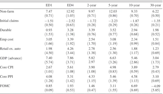
Table 2 repeats the same exercise that was carried out in Table 1, this time using heteroskedasticity-based identification. It is striking that all the coefficients are much larger when identification via heteroskedasticity is employed compared to OLS, which would be the natural effect of correcting for attenuation bias in the measurement error model. Therefore, a possible interpretation of this finding is that headline news is indeed measured with substantial error, leading to attenuation bias, and that heteroskedasticity-based identification is robust to these problems. This is the interpretation offered by Rigobon and Sack (2008). But σ η2 would have to be
Table 2—Heteroskedasticity-Based Estimates Following Rigobon (2003) and Rigobon and Sack (2004, 2005, 2008)
ED1 ED4 2-year 5-year 10-year 30-year
Non-farm 7.47 12.92 9.97 12.03 9.33 6.22 (0.71) (1.03) (0.71) (0.86) (0.70) (0.50) Initial claims − 1.51 − 2.52 − 1.72 − 2.23 − 1.87 − 1.35 (0.50) (0.63) (0.28) (0.29) (0.26) (0.21) Durable 0.93 3.28 3.39 3.52 2.94 1.98 (1.53) (1.38) (0.76) (0.77) (0.68) (0.52) Emp cost 3.05 3.39 2.54 3.08 2.34 1.51 (1.66) (1.92) (1.70) (1.19) (0.99) (0.84)
Retail ex. auto 1.98 4.26 2.78 2.56 1.88 1.23
(4.50) (3.44) (1.38) (1.30) (1.17) (0.69) GDP (advance) 7.40 7.86 5.82 6.63 5.46 3.04 (5.74) (3.71) 2.97 (3.26) (2.86) (1.73) Core CPI 2.67 5.61 3.90 4.98 3.89 2.79 (1.01) (1.08) (1.08) (0.83) (0.59) (0.43) Core PPI 4.08 5.31 4.33 5.46 4.58 3.10 (1.28) (1.42) (1.15) (1.39) (1.13) (0.69) FOMC 0.85 1.93 1.46 3.11 6.69 − 4.09 (0.09) (0.53) (0.47) (1.55) (8.69) (5.85)
Notes: Asymptotic standard errors are in parentheses. Macroeconomic surprises are normalized by their respective standard deviations. Monetary policy surprises are in basis points. Responses of ED1, ED4, 2-year, 5-year, 10-year, and 30-year yields are in basis points. The sample is 1992–2018 for macroeconomic announcements, 1992–2007 for monetary policy surprises.
large compared to σ ∗2 for this to be true, and we argue in Section IIIB that this is not
the case.
In this paper, we offer a different interpretation, more in line with the evidence showing the broad efficiency of survey expectations of data releases. We argue that survey expectations are measuring headline surprises correctly but instead there are surprise components in news announcements that are not directly observed by the econometrician, which have important effects on asset prices. Our reasons for think-ing along these lines, and the proposed methodology to accommodate this feature of the data, are presented in the next section.
II. Partially Measured News and Heteroskedasticity-Based Identification We recognize that data releases are elaborate and multidimensional. The “news” that is captured in OLS-based event studies is only headline news, i.e., the devia-tion of the headline number from its survey expectadevia-tion. The survey expectadevia-tions are well measured and usually pass standard forecast rationality tests. Gürkaynak and Wolfers (2007) find that survey-based forecasts are roughly comparable in effi-ciency to market-based ones, and we expand on this argument in Section III.
However, it remains the case that the headline news is only part of news releases. Releases also contain other information such as revisions to past data and informa-tion on subcomponents. For example, the GDP release reports the contribuinforma-tions of different expenditure items, and markets may react differently to increases in GDP driven by gross fixed capital formation versus inventory increases. Some releases contain a discussion of current conditions and even forecasts. The FOMC release is the obvious example, where the statement has for some time garnered more atten-tion than the immediate policy setting. Yet in terms of “news,” only the headline is observable as there are surveys for these numbers alone. The balance of the news in the release is unobservable to the econometrician, but elicits a market response as well. We argue that this is why the R 2 s of OLS-based event studies are not very high.
The regression only captures the contribution of the headline news to the variance of asset prices and effects of all other news in the same release show up in the residual.
Notice that under this interpretation, the OLS-based event study answers a nar-rowly defined question correctly: it determines the relationship between the head-line news (but not the whole news release) and the asset price in question. The heteroskedasticity-based estimator instead allows the news to be unobservable and conditions only on the time of the data release. To the extent that news is mul-tidimensional, the increase in variance at the time of the release is due to more than the headline surprise. The heteroskedasticity-based estimator captures the asset price response to the news release as a whole, not only to the headline num-ber. This, rather than sizable measurement error in survey expectations, is why the heteroskedasticity-based estimator always finds larger asset price response coef-ficients. In the next section, we show this analytically, and bring direct evidence to verify that heteroskedasticity-based estimator, along with the headline surprise effects, captures the effects of non-headline component of the release.
We therefore posit that a complete understanding of yield changes in news release event windows is possible, using OLS to partial out the effects of the observable news on the asset prices, and then using heteroskedasticity-based identification to
learn the effect of non-headline, unobservable news in the data release. This could be done in two steps, with heteroskedasticity-based identification applied to resid-uals from the OLS regression3 but we instead introduce an efficient, one-step
esti-mator via the Kalman filter. This has the useful by-product of giving an estimate of the unobserved news component in any given data release, which is not directly available from identification through heteroskedasticity.
We let y t denote the 6 × 1 vector of yield changes (of maturities studied in Tables 1
and 2) from 8:25am to 8:45am. Some days have macroeconomic announcements at
8:30am, while others do not, but all the macroeconomic announcements that we consider come out at 8:30am. In the implementation for FOMC policy surprises, we let y t denote the 6 × 1 vector of yield changes from 2:10pm to 2:30pm (incorporating
some minor deviations of timing to accommodate FOMC announcements times).
Monetary policy dates and times are from Gürkaynak, Sack, and Swanson (2005)
up to December 2004, and from Federal Reserve Board (2020) since then. Data
from these intradaily windows are included regardless of whether they contain an announcement.
The model that we specify is then
(7) y t = β ′ s t + γ ′ d t f t + ε t ,
where s t is the vector of observable surprises in macroeconomic or monetary policy announcements,4 d
t is a dummy that is 1 if there is an announcement in that window and 0 otherwise, f t is an i.i.d. N
(
0, 1)
latent variable that is common to all releases, and ε t is i.i.d. normal with mean zero and diagonal variance-covariance matrix. The sample period and the data used to measure surprises remain the same.Equation (7) would essentially collapse to the standard OLS event study regres-sion if the ft term were dropped, and to a heteroskedasticity-based estimator if the st term were dropped. As it stands, this equation can be estimated by maximum likeli-hood via the Kalman filter.5
A. Kalman Filter and Identification
In our Kalman filter-based method, equation (7) is the measurement equation and the i.i.d. sequence of { f t } is the state.6 The Kalman filter provides an orthogonal
decomposition
(
s t ⊥ f t)
consistent with the idea that f t can also be recovered by heteroskedasticity-based methods from OLS ( y t on s t ) residuals, where these resid-uals would be orthogonal to observable surprises. Thus in essence, f t is identified by the heteroskedasticity of the OLS residuals, where identification requires d t being equal to 1 for some but not all dates (having both event and nonevent dates in the3 We report the results from doing this in online Appendix Section B. 4 s
t is set to 0 for any announcement that does not take place in that window.
5 Maximum likelihood estimates are obtained via the EM algorithm. Our code can handle any number of
releases, asset price changes, and latent factors and is made available for others to use.
6 This is an unusual use of the Kalman filter as it is usually employed for data that are serially correlated. The
i.i.d. latent variable (surprises by definition will be uncorrelated) is a special case that can be written in state-space form and is recoverable by the Kalman filter.
sample). The variance of f t is normalized to unity as otherwise γ would be identified only up to scale.
The Kalman filter estimates the latent factor f t and the effects of the latent and observable ( s t ) surprises on yields efficiently. Using a vector of yields is not nec-essary. As every yield is heteroskedastic, we could estimate f t from any one of them: homoskedasticity of ϵ t and heteroskedasticity of f t identifies them separately (up to scale) with a non-degenerate dt distribution. Thus, we are not relying on a cross-sectional covariance in the yt vector for identification,7 and indeed the β
coef-ficient estimates are the same regardless of whether equation (7) is estimated jointly or equation-by-equation. (SUR coefficients are the same as equation by equation OLS when right-hand-side covariates are the same, as is the case here.)
Given the understanding of partially observed, multidimensional data releases presented in this paper, multiple yields and the cross-sectional variance of y t can also be used to identify the latent factor and its effects in a two-step procedure, by first regressing the yield changes on surprises and then extracting the first prin-cipal component from OLS residuals. But our Kalman filter approach is prefera-ble for three reasons. First, and most importantly, the two-step procedure that does not employ nonevent window information cannot disentangle common yield curve movements that would be present even without an announcement from those caused
by the announcement, whereas our Kalman-filter based method can do this (see
Section IV). Second, in contrast to the Kalman filter, two-step methods are ineffi-cient. And third, the two-step method does not work with only a single asset, unlike what we propose here. Online Appendix Section D presents our implementation of the Kalman filter in this context, showing algebraically how the system is identified.
B. Baseline Results
Table 3 reports the results, along with R 2 values from the regressions of y
t on s t alone, and from regressions augmented with the Kalman-smoothed estimate of f t in equation (7), around announcement times. The headline surprise alone explains less than 40 percent of announcement-window variation in each of the yields considered here, as in Table 1. Augmenting the regression with one latent factor brings the explained share up to over 90 percent. We can explain about all of the movements in the term structure of interest rates around news announcements with the headline surprise and one latent factor. Inclusion of the latent factor makes little difference to the estimated coefficients on the headline surprises due to orthogonality, although it does reduce the error variance and hence the standard errors.
The specification in equation (7) implies that the latent factor has the same loadings for all announcement types and it is worth noting that the R2 values are
so high despite this constraint. The releases are clearly heteroskedastic, with the employment report creating the largest variance, and so the model is literally mis-specified: the draws of f t on employment report days have sample variance greater than 1. That does not prevent the model from fitting well, which means that different announcements have similar relative effects on different points of the yield curve.
7 We will use cross-sectional covariance and will need multiple assets in Section IVB when we also allow for a
Nonetheless, we can extend the model to incorporate release-specific factors, spec-ifying instead that
(8) y t = β ′ s t +
∑
i=1I
d it γ i f it + ε t ,
where d it is a dummy that is 1 if an announcement of the i th type comes out in win-dow t and 0 otherwise and I is the number of latent factors. Because they always come out concurrently, non-farm payroll/unemployment/average hourly earnings, retail sales/retail sales ex autos, core PPI/PPI, and core CPI/CPI surprises each share a single latent factor, and so there are eight latent macroeconomic announce-ment factors, even though there are 13 8:30am macroeconomic announceannounce-ments.
Table 3—Estimates of Equation (7)
ED1 ED4 2-year 5-year 10-year 30-year
Non-farm 2.87 5.66 4.46 5.26 3.97 2.41 (0.16) (0.24) (0.20) (0.21) (0.16) (0.11) Initial claims − 0.30 − 0.71 − 0.56 − 0.6 − 0.53 − 0.32 (0.02) (0.04) (0.03) (0.03) (0.03) (0.02) Durable 0.38 0.86 0.66 0.82 0.58 0.37 (0.06) (0.10) (0.08) (0.09) (0.08) (0.05) Emp cost 0.68 1.49 1.14 1.48 1.15 0.74 (0.10) (0.22) (0.17) (0.21) (0.16) (0.11) Retail 0.31 0.74 0.60 0.54 0.38 0.14 (0.09) (0.12) (0.09) (0.11) (0.10) (0.07)
Retail ex. auto 0.40 0.91 0.84 1.16 0.92 0.70
(0.07) (0.12) (0.10) (0.11) (0.09) (0.07) GDP 0.66 1.61 1.18 1.59 1.21 0.70 (0.07) (0.17) (0.12) (0.15) (0.12) (0.08) CPI 0.01 − 0.07 − 0.02 0.10 0.15 0.19 (0.05) (0.11) (0.08) (0.10) (0.08) (0.06) Core CPI 0.72 1.66 1.24 1.56 1.27 0.81 (0.06) (0.10) (0.09) (0.10) (0.08) (0.06) PPI 0.10 0.25 0.18 0.18 0.23 0.16 (0.05) (0.08) (0.07) (0.08) (0.06) (0.04) Core PPI 0.61 1.05 0.77 1.03 0.89 0.68 (0.06) (0.10) (0.08) (0.08) (0.07) (0.05) Unemp − 1.23 − 2.04 − 1.64 − 1.70 − 1.18 − 0.68 (0.11) (0.18) (0.14) (0.15) (0.12) (0.08) Hourly earnings 0.88 1.84 1.44 2.02 1.61 0.97 (0.12) (0.17) (0.14) (0.17) (0.13) (0.09) FOMC 0.57 0.43 0.28 0.14 0.03 −0.02 (0.04) (0.04) (0.04) (0.04) (0.02) (0.01) Factor 1.37 3.14 2.42 2.94 2.28 1.46 (0.03) (0.05) (0.04) (0.04) (0.03) (0.02) R 2 no factor 0.40 0.36 0.37 0.36 0.34 0.30 R 2 with factor 0.73 0.92 0.94 0.98 0.96 0.87
Notes: Standard errors are in parentheses. Macroeconomic surprises are normalized by their respective standard deviations. Monetary policy surprises are in basis points. Responses of ED1, ED4, 2-year, 5-year, 10-year, and 30-year yields are in basis points. The sample is 1992–2018 for macroeconomic announcements, 1992–2007 for monetary policy surprises. The factor is estimated via the Kalman Filter using changes in asset prices around mac-roeconomic and FOMC releases. The R2 values are those of announcement day yields using (i) only headline
Including the monetary policy factor, in total we have nine release related factors to be estimated. The factors
{
f it}
iI=1 are all standard normal and are independent over time and independent of each other. This extended model can also be estimated by maximum likelihood via the Kalman filter. The results are reported in Table 4. The coefficient estimates on the headline surprises are similar to those in Tables 1 and 3.Table 4 also includes the R 2 values from regressions of elements of y
t on s t alone, and from regressions augmented with the Kalman smoothed estimates of the latent factors associated with macro announcements. Incorporating the macro-factors again increases the R 2 values from below 40 percent to above 90 percent for most
maturities. The R 2 values are similar to the single factor case, even though the single
factor model is nested in equation (8). (The R 2 would not be 1 because the usual
market noise, as measured by nonevent window variance of yields, is still in the data.)
In the next two sections we provide a deeper understanding and better intuition for these issues, as well as presenting extensions.
III. Discussion: Understanding the Latent Factor
In this section we study the relationship between measurement error, latent fac-tors, OLS, and heteroskedasticity-based estimators. To do so, we analytically explore the implications of different modeling assumptions about the data-generating pro-cess on OLS and heteroskedasticity-based estimates and turn to empirical evidence to see which of these are consistent with the data. We then study the properties of the latent factor and show that it is indeed related to non-headline news and discuss how these results help improve our understanding of yield curve movements.
A. A General Model
The heteroskedasticity-based parameter estimates are larger in absolute value than their OLS counterparts but this is consistent with either attenuation bias from measurement error in the headline surprises or the presence of an unobservable latent factor. The difference in estimates, by itself, does not distinguish between the measurement error and unobserved surprises alternatives.8
To show this formally, we consider a general model which incorporates both measurement error and an unobservable latent factor, nesting both cases. Here we discuss the case with scalars for ease of notation. The intuition is identical when y t is a vector, as employed in our application of the Kalman filter. The model is
y t = β s t∗ + γ d t f t + ε t , s t = s t∗ + η t ,
8 Another alternative, also discussed by Rigobon and Sack, is that correctly measured news is imperfectly
infor-mative about an underlying state of the economy and the market reaction is to the update of that state. This may indeed be the case and that interpretation is consistent with ours as the OLS coefficient would then reflect the mapping between the state and the headline news, and the orthogonal latent factor would be statistically significant and would improve the R 2 in yield reaction regressions only if non-headline news in the release are independently
Table 4—Estimates of Equation (8)
ED1 ED4 2-year 5-year 10-year 30-year
Non-farm 2.87 5.66 4.46 5.27 3.97 2.41 (0.16) (0.24) (0.20) (0.21) (0.16) (0.11) Initial claims − 0.31 − 0.72 − 0.58 − 0.68 − 0.55 − 0.33 (0.02) (0.03) (0.02) (0.03) (0.02) (0.02) Durable 0.40 0.88 0.69 0.85 0.60 0.39 (0.06) (0.11) (0.09) (0.10) (0.08) (0.05) Emp cost 0.68 1.47 1.12 1.46 1.13 0.73 (0.10) (0.22) (0.17) (0.21) (0.16) (0.11) Retail 0.25 0.61 0.49 0.40 0.27 0.06 (0.08) (0.10) (0.08) (0.09) (0.08) (0.06)
Retail ex. auto 0.44 1.02 0.92 1.26 1.00 0.76
(0.07) (0.12) (0.09) (0.11) (0.09) (0.06) GDP 0.64 1.58 1.16 1.56 1.18 0.68 (0.07) (0.15) (0.10) (0.13) (0.11) (0.07) CPI 0.01 −0.08 −0.02 0.10 0.15 0.19 (0.05) (0.11) (0.08) (0.10) (0.08) (0.06) Core CPI 0.67 1.57 1.17 1.49 1.22 0.78 (0.05) (0.10) (0.08) (0.10) (0.08) (0.06) PPI 0.11 0.28 0.20 0.22 0.26 0.18 (0.05) (0.09) (0.07) (0.08) (0.06) (0.04) Core PPI 0.63 1.07 0.80 1.06 0.91 0.70 (0.07) (0.10) (0.08) (0.09) (0.07) (0.05) Hourly earnings 0.88 1.84 1.44 2.02 1.61 0.97 (0.12) (0.17) (0.14) (0.17) (0.13) (0.09) Unemp − 1.23 − 2.04 − 1.64 − 1.70 − 1.18 − 0.68 (0.11) (0.18) (0.14) (0.15) (0.12) (0.08) FOMC 0.57 0.42 0.28 0.14 0.03 −0.02 (0.04) (0.04) (0.04) (0.04) (0.02) (0.01) f CPI,t 1.10 2.63 2.08 2.63 2.10 1.46 (0.05) (0.09) (0.07) (0.08) (0.06) (0.05) f Durable,t 0.81 1.99 1.51 1.85 1.49 0.98 (0.06) (0.10) (0.06) (0.06) (0.04) (0.03) f EmpCost,t 0.81 2.52 2.09 2.70 2.10 1.45 (0.13) (0.25) (0.19) (0.27) (0.23) (0.16) f GDP,t 1.47 3.08 2.23 2.73 2.18 1.35 (0.31) (0.23) (0.19) (0.19) (0.14) (0.08) f Claims,t 0.64 1.53 1.14 1.45 1.19 0.80 (0.03) (0.05) (0.03) (0.03) (0.02) (0.02) f NonFarm,t 2.57 5.68 4.42 5.50 4.23 2.67 (0.11) (0.17) (0.13) (0.13) (0.10) (0.08) f PPI,t 1.28 2.44 1.97 2.37 1.95 1.35 (0.09) (0.10) (0.07) (0.09) (0.08) (0.05) f Retail,t 1.50 2.94 2.28 2.52 1.92 1.18 (0.15) (0.17) (0.10) (0.10) (0.07) (0.05) f FOMC,t 2.19 6.17 4.58 5.11 3.58 2.02 (0.18) (0.33) (0.24) (0.32) (0.22) (0.15) R 2 no factor 0.40 0.36 0.37 0.36 0.34 0.30 R 2 release factors 0.73 0.93 0.94 0.98 0.96 0.88
Notes: Standard errors are in parentheses. Macroeconomic surprises are normalized by their respective standard deviations. Monetary policy surprises are in basis points. The R2 values reported are those for announcement day
yields using (i) only headline surprises, (ii) headline surprises and latent factors. The sample is 1992–2018 for mac-roeconomic announcements, 1992–2007 for monetary policy surprises.
where y t is a scalar log return or yield change, s t is the scalar observed surprise, s t∗ is the true headline surprise, d t is a dummy that is 1 on an announcement day and 0 otherwise, f t is an i.i.d. N
(
0, 1)
latent variable, and ε t and η t are processes measur-ing noise in yields and measurement error of the headline surprise. We assume that s t∗ , ε t , and η t are i.i.d., mutually uncorrelated, have mean zero, and variances σ ∗2 , σ ε2 ,and σ η2 , respectively. To estimate β , the parameter of interest in event studies, using
OLS and identification through heteroskedasticity, we need the variance-covariance matrices for event ( Ω E ) and nonevent ( Ω NE ) windows:
Ω E =
(
β 2 σ ∗ 2 + γ 2 + σ ε 2 β σ ∗2 . σ ∗2 + σ η2)
, Ω NE = ( σ ε 2 0 0 0) . In this general model, the OLS estimate for β isβ ˆ OLS = _____
[
Ω ˆ E]
1,2[
Ω ˆ E]
2,2and the identification through heteroskedasticity estimate of β is
β ˆ HET =
[
Ω ˆ E]
1,1 −[
Ω ˆ NE]
1,1 _____________[
Ω ˆ E]
1,2 .This general model collapses to a model with no latent factor if γ = 0 and it collapses to the no measurement error case (the case we argue for in this paper) when σ η2 = 0 . In the general model, as shown in online Appendix Section C, the
probability limits of the two estimators are
β ˆ OLS → β
(
1 − σ η 2 _ σ ∗2 + σ η2)
and β ˆ HET → β (1 + γ 2 _ β 2 σ * 2 ) .If there is neither a latent factor ( γ = 0 ) nor measurement error in the surprise ( σ η2 = 0 ), the OLS and heteroskedasticity based estimators both uncover the true β
and should coincide. However, as Tables 1 and 2 show, these are significantly differ-ent from each other, implying that this is not the relevant case.
With a latent factor, the heteroskedasticity-based estimator is biased away from zero. Note that the term γ 2 /( β 2 σ
∗
2 ) is proportional to the variance share of the latent
factor in the event window changes of yields. As the relative variance share of the latent factor increases ( non-headline news carries more information affecting
yields), the bias of the heteroskedasticity-based estimator for the headline effect increases.9
With measurement error, the OLS estimate will be biased toward zero because of classical attenuation bias. This bias is proportional to the share of measurement error in total variance of the observed surprise, σ η2 /( σ
∗ 2 + σ
η 2 ) .
Except for the case where there is no latent factor and no measurement error in the surprise, the probability limit of the heteroskedasticity-based estimator will always be larger than the OLS estimate in absolute value, as we find in the data. However, this could be because of a latent factor ( γ ≠ 0 ), or measurement error ( σ η2 ≠ 0 ), or both. It is this observational equivalence that makes it impossible to
judge whether OLS is consistent by only looking at the difference between the OLS and heteroskedasticity-based estimates.10 One has to take a stance on the extent of
measurement error. Given the observed difference between the two estimators, that stance is consequently also on the presence of unobserved surprises and the consis-tency of the heteroskedasticity-based estimator.
We argue that measurement error in survey-based surprises is negligible,
so σ η2 ≈ 0 , and therefore β ˆ OLS is consistent, whereas β ˆ HET is not. We shall do this in Subsection IIIB, by bringing in data from economic derivatives to show that mea-surement error in the survey-based surprises is likely to be negligible for event stud-ies. As further corroborating evidence, the bias term for heteroskedasticity-based identification when there is a latent factor, discussed above, shows that the differ-ence between β ˆ HET and β ˆ OLS should be larger when |γ| is larger, that is when events have larger non-headline components. To examine this, in Subsection IIIC, we shall compare monetary policy announcements with and without accompanying state-ments. We will show that heteroskedasticity-based estimates are closer to the OLS counterparts on days without monetary policy statements compared to the days with statements.
B. Quality of Survey Expectations
The surveys used in event studies are those of news releases that are to take place very soon, no longer than a week after the time of the survey. And the “event” is the release of information on something that has already taken place. Hence, these expectations are not necessarily subject to the anomalies often reported in analysis of long-term expectations (Fuhrer 2017).11
Nonetheless, three areas of concern remain: (i) the survey expectation may be stale, i.e., there may be incoming news between a respondent’s reporting of her expectation and the releases, which change her expectations, (ii) respondents may not have sufficient skin in the game, and (iii) respondents may have an incentive to be right in the extreme case, not on average, therefore reporting numbers closer to the tails rather than their true expectations, especially if their predictions are not
9 As the variance of the latent factor σ f
2 is normalized to unity, γ 2 itself is the measure of variance due to the
latent factor.
10 It is also the reason why measurement error in the observable and a latent factor cannot simultaneously be
estimated.
11 Notwithstanding these anomalies, Ang, Bekaert, and Wei (2007) show that survey expectations remain the
anonymous. We argue that while these concerns sound relevant, in practice survey expectations work remarkably well and are not subject to large measurement errors.
To do so, we compare the survey-based expectations to timely market-based expectations. The latter data come from Gürkaynak and Wolfers (2007), who ana-lyze the market for Economic Derivatives. This was a market, now defunct, where Deutsche Bank and Goldman Sachs allowed trades of binary options on news releases about half an hour before the release itself.12 Market-based expectations of
data releases are not subject to any of the potential measurement error problems that survey-based ones might be. The market operates minutes before the data release, hence there is no scope for staleness; the traders do have skin in the game as they bet on their expectations; and since the market returns are anonymous they have no special incentive to get low probability events right.
We construct market- and survey-based expectations and news surprises based on these and directly test whether there is measurement error in survey-based expec-tations by comparing the market responses to the two surprise measures. If there is sizable measurement error in survey-based surprises, event study coefficients based on these should be significantly smaller than coefficients based on Economic Derivatives-based surprises, which are not subject to measurement error.
We run SUR regressions for the four releases covered by Economic Derivatives (Nonfarm payrolls, NAPM, Retail Sales ex-Autos, and Initial Claims) of the form
(9) y t =
∑
i=1 4 θ is S itSURVEY + ε t , (10) y t =∑
i=1 4 θ im S it ECON-DERIV + ε t , where S itSURVEY and Sit
ECON-DERIV are surprises where expectations are measured
using surveys and Economic Derivatives, respectively. Measurement error in sur-vey expectations will lead to smaller θ s compared to θ m . Table 5 reports the results as well as the joint test of the hypothesis that θ is = θ
i
m for all i . It is striking that while all estimated θ is s are somewhat smaller than corresponding θ
i
m s (consistent with minor classical measurement error) the differences in point estimates are small and in no cases individually or jointly statistically significant.13 Thus we conclude
that survey expectations capture market expectations extremely well. Even if one attributes all of the difference between point estimates to measurement error, the differences are on the order of 5 to 15 percent, an order of magnitude smaller than the gap between OLS and heteroskedasticity-based estimates shown in Tables 1 and 2. These substantial differences cannot be predominantly due to measurement error in surveys and resulting attenuation bias in the coefficients.
12 These call options paid off if the release came in at or above the buyer’s strike price. Gürkaynak and Wolfers
(2007) describe the market and these options, as well as the methodology to use them to construct risk neutral probability density functions of market perceived data release outcomes.
13 In his discussion of Gürkaynak and Wolfers (2007), Carroll (2007) notes how the survey- and market-based
expectations are remarkably similar to each other in terms of first moments. This is consistent with what we find here but the similarity is actually stronger: for almost every single event, the market- and survey-based expectations are very close to each other.
C. Comparison of OLS and Heteroskedasticity-Based Estimates
A well-studied and well-understood case of multidimensional data release is that of FOMC announcements, which contain both the interest rate decision and an accompanying statement providing information on the future course of interest rates. This is a case we will return to in more detail but here we will exploit the fact that FOMC releases did not always contain statements. Until 1994, the FOMC did not issue statements and until 1999 statements were only issued when the policy rate was changed.
Under the measurement error model, the difference between OLS and heteroskedasticity-based estimators should not depend on the presence of an accom-panying statement. If on the other hand, as we suggest, heteroskedasticity-based identification provides the asset price response to the whole “event” rather than just the headline, the difference between the two measures should be larger when the non-headline component is more important, i.e., γ is larger. Increasing the importance of non-headline news is exactly what the FOMC did when it began to issue state-ments. So, if our conjecture is correct, the coefficient estimates of the impact of FOMC announcements on yields measured by OLS and heteroskedasticity-based
Table 5—Seemingly Unrelated Regression (SUR) Results for ED1, ED4, and On-the-Run 2-, 5-, 10-, and 30-Year Yields
Non-farm Initial claims NAPM Retail Obs. R 2 p-value ( χ 2 )
ED1 Auction 1.40 −0.12 0.05 0.19 152 0.31 0.82 (0.19) (0.13) (0.12) (0.19) Survey 1.33 −0.11 0.04 0.17 152 0.28 (0.20) (0.13) (0.12) (0.19) ED4 Auction 6.99 −0.53 0.43 0.40 153 0.48 0.87 (0.63) (0.44) (0.43) (0.65) Survey 6.75 −0.51 0.37 0.38 153 0.45 (0.66) (0.46) (0.45) (0.68) Two-year Auction 4.72 −0.38 0.36 0.35 153 0.42 0.87 (0.49) (0.34) (0.32) (0.50) Survey 4.54 −0.36 0.30 0.33 153 0.38 (0.52) (0.36) (0.34) (0.53) Five-year Auction 5.62 −0.47 0.54 0.49 153 0.45 0.78 (0.54) (0.37) (0.37) (0.56) Survey 5.39 −0.44 0.45 0.45 153 0.41 (0.57) (0.40) (0.39) (0.39) Ten-year Auction 4.37 −0.37 0.42 0.41 153 0.43 0.88 (0.45) (0.31) (0.30) (0.46) Survey 4.22 −0.35 0.36 0.38 153 0.4 (0.47) (0.33) (0.32) (0.48)
Notes: Auction are the coefficients for the market based surprises and Survey are MMS/Action Economics sur-vey-based surprise coefficients. Standard errors are in parentheses; p-value is the joint test statistic of equality between auction and survey estimates. The sample is from October 2002 to July 2005.
estimators should be closer for a sample of events consisting of policy actions only, than for a sample consisting of announcements that also have statements providing information on the policy path.
For monetary policy surprises, as before, we follow the standard procedure and use federal funds futures-based surprises as suggested by Kuttner (2001). Table 6 shows that when statements do not accompany the policy rate decision, the OLS and heteroskedasticity-based estimates of the asset price reactions are quite similar, though the OLS estimates are smaller due to market participants’ inference of infor-mation even in the absence of formal statements. But for the sample that includes statements the heteroskedasticity-based estimator yields a reaction coefficient that is two to 400 times larger than the OLS estimator.
What is striking here is not that OLS coefficients are a little smaller and sta-tistically less significant in the latter sample. This is due to the dearth of policy action surprises in the twenty-first century, when policy actions were usually
sig-naled ahead of the FOMC meeting date (Swanson 2006). What is noteworthy is
the increase in the spread between OLS and heteroskedasticity-based estimators, and the fact that the spread becomes significantly more pronounced as maturity increases. The last row of the table shows that the increase in the difference is sta-tistically significant. This is exactly what one would expect to find based on our conjecture: the presence of a statement will increase the distance between OLS and heteroskedasticity-based estimates for all maturities but as the statement is more informative for longer maturities14 the heteroskedasticity-based estimator will find
even larger coefficients for those maturities.
14 The literature, described in the next section, finds that quantifying the statement can explain the movement in
longer maturities, whereas short maturities are more responsive to the immediate policy action.
Table 6—OLS and Heteroskedasticity-Based Results for the Days with and without Monetary Policy Statements
ED1 ED4 2-year 5-year 10-year 30-year
FOMC full sample
OLS 0.57 0.44 0.28 0.14 0.03 −0.02 (0.07) (0.1) (0.09) (0.07) (0.04) (0.02) ID HET 0.85 1.93 1.46 3.11 6.69 −4.09 (0.09) (0.53) (0.47) (1.55) (8.69) (5.85) FOMC no statement OLS 0.76 0.84 0.55 0.25 0.09 0.04 (0.20) (0.29) (0.18) (0.15) (0.09) (0.04) ID HET 0.88 1.02 0.65 0.05 −0.13 −0.28 (0.11) (0.16) (0.09) (0.50) (0.54) (0.64) FOMC statement OLS 0.55 0.40 0.25 0.13 0.03 −0.02 (0.08) (0.09) (0.09) (0.07) (0.05) (0.02) ID HET 0.85 2.11 1.61 3.56 8.45 −3.56 (0.10) (0.65) (0.60) (1.89) (13.28) (4.30)
Equivalence test for statement and non-statement days
OLS 0.97 1.46 1.47 0.70 0.61 1.36
ID HET 0.18 −1.61 −1.57 − 1.79 −0.65 0.75
Thus, by studying the FOMC announcement dates, we conclude that the heteroskedasticity-based estimator provides a convolution of the asset price responses to the headline and non-headline components of news, whereas our partial observability-based Kalman filtering methodology provides asset price responses to headline news and the latent non-headline news component separately. An addi-tional benefit is that this method estimates the latent component directly, and allows it to be given an economic interpretation.
It can be shown, as we do in online Appendix Section C, that the heteroskedasticity-based estimator is essentially the sum of the OLS response to the observables and the response to the latent variable that can be extracted from the residuals. The method that we developed does this efficiently, in one step.
D. Interpreting the Latent Factor
So far we have focused on the relationship between the heteroskedasticity-based, OLS and Kalman filter-based estimators and showed that the discrepancy between the two is better understood as arising from the presence of unobserved surprises in releases rather than measurement error in observed surprises. We also showed that a single factor estimated using the Kalman filter along with observable headline surprises is sufficient to explain the variation in asset prices around macroeconomic news events. In this subsection, we closely examine the economic interpretation of that latent factor.
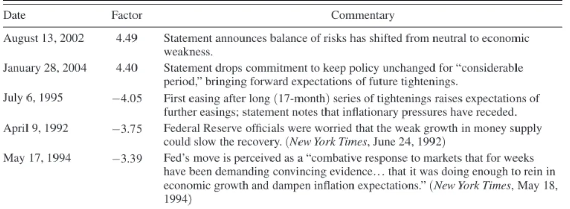
Table 7 lists the five largest readings of the latent factor in FOMC announce-ment windows and shows that based on the comannounce-ments in the financial press, these are indeed days of well-known “statement surprises.” Monetary policy statement surprises are well understood and it is reassuring that the latent factor we extract behaves as expected. Non-headline surprises in other macroeconomic data releases are much less well understood, not only in the academic literature but also in the financial press. Thus, the financial press reports of non-headline items are often boil-erplate, listing the numbers without much commentary, so doing the same exercise
Table 7—FOMC Commentary
Date Factor Commentary
August 13, 2002 4.49 Statement announces balance of risks has shifted from neutral to economic weakness.
January 28, 2004 4.40 Statement drops commitment to keep policy unchanged for “considerable period,” bringing forward expectations of future tightenings.
July 6, 1995 −4.05 First easing after long (17-month) series of tightenings raises expectations of further easings; statement notes that inflationary pressures have receded. April 9, 1992 −3.75 Federal Reserve officials were worried that the weak growth in money supply
could slow the recovery. (New York Times, June 24, 1992)
May 17, 1994 −3.39 Fed’s move is perceived as a “combative response to markets that for weeks have been demanding convincing evidence… that it was doing enough to rein in economic growth and dampen inflation expectations.” (New York Times, May 18, 1994)
Notes: Table shows the 5 largest (absolute) values of the latent factor monetary policy announcements with asso-ciated dates and the summary of the statements. January 28, 2004, August 13, 2002, July 6, 1995 commentary are from Gürkaynak, Sack, and Swanson (2005).
for macroeconomic data releases is not possible. We therefore do the next best thing and create pseudo-unobservable surprises.
To verify that our method indeed picks up unsurveyed news in data releases we take the observable surprises in the employment report—nonfarm payrolls, unem-ployment rate, and hourly earnings—and drop the nonfarm payrolls surprise from the data, treating it as if this component of the employment report is not surveyed and hence its surprise is unobservable to the econometrician.15 We then look at the
correlation between the latent factor we extract on employment report release days and the surprise that we have excluded from the data. Figure 3 shows the results of the exercise. The correlation between the nonfarm payrolls surprise and the latent factor extracted from the factor model is striking. The estimated latent factor indeed tracks the surprise as measured by the survey. The correlation is not perfect because the truly unobserved surprises are also being picked up by the factor, but as the nonfarm payrolls surprise has a large variance share, this is closely tracked by the estimated latent factor.
We have shown that the financial market responses to news announcements depend on surprises, some of which are observed by both market participants and the econometrician, and some of which are observed by market participants but not directly by the econometrician. These responses to both kinds of news may per-haps be due to behavioral finance effects; market participants extracting information on an underlying state of the economy from the releases; or in the case of FOMC announcements, non-overlapping information sets between FOMC and the public. These are issues that go to the heart of financial and macroeconomic research that
15 Doing this for the other two observed surprises produces similar results but since nonfarm payrolls surprises
elicit the largest yield curve responses, visually this case is easier to present.
corr = 0.70 −4 −2 0 2 4 1995 2000 2005 2010 2015 Factor
Non-farm payroll surprise (standardized)
Figure 3
Note: Shows the time series of nonfarm payrolls surprise and the latent factor estimated around employment report days treating nonfarm payrolls surprise as unobservable.