LOCATION BASED MULTICAST ROUTING
ALGORITHMS FOR WIRELESS SENSOR
NETWORKS
a thesis
submitted to the department of computer engineering
and the institute of engineering and science
of bilkent university
in partial fulfillment of the requirements
for the degree of
master of science
By
Hakkı BA ˘
GCI
August, 2007
Asst. Prof. Dr. ˙Ibrahim K¨orpeo˘glu(Advisor)
I certify that I have read this thesis and that in my opinion it is fully adequate, in scope and in quality, as a thesis for the degree of Master of Science.
Dr. Cengiz C¸ elik
I certify that I have read this thesis and that in my opinion it is fully adequate, in scope and in quality, as a thesis for the degree of Master of Science.
Prof. Dr. Adnan Yazıcı
Approved for the Institute of Engineering and Science:
Prof. Dr. Mehmet B. Baray Director of the Institute
ABSTRACT
LOCATION BASED MULTICAST ROUTING
ALGORITHMS FOR WIRELESS SENSOR NETWORKS
Hakkı BA ˘GCI
M.S. in Computer Engineering
Supervisor: Asst. Prof. Dr. ˙Ibrahim K¨orpeo˘glu August, 2007
Multicast routing protocols in wireless sensor networks are required for sending the same message to multiple different destination nodes. Since most of the time it is not convenient to identify the sensors in a network by a unique id, using the location information to identify the nodes and sending messages to the target locations seems to be a better approach. In this thesis we propose two different distributed algorithms for multicast routing in wireless sensor networks which make use of location information of sensor nodes. Our first algorithm groups the destination nodes according to their angular positions and sends a message toward each group in order to reduce the number of total branches in multicast tree which also reduces the number of messages transmitted. Our second algorithm calculates an Euclidean minimum spanning tree at the source node by using the positions of the target nodes. According to the calculated MST, multicast message is forwarded to destination nodes. This helps reducing the total energy consumed for delivering the message to all target nodes since it tries to minimize the number of transmissions. We compare these two algorithms with each other and also against another location based multicast routing protocol called PBM according to success ratio in delivery, number of total transmissions, traffic overhead and average end to end delay metrics. The results show that algorithms we propose are more scalable and energy efficient, so they are good candidates to be used for multicasting in wireless sensor networks.
Keywords: Wireless Sensor Networks, Location Based Multicasting, Geographic Routing.
C
¸ OKLU G ¨
ONDER˙IM YOL BULMA ALGOR˙ITMALARI
Hakkı BA ˘GCI
Bilgisayar M¨uhendisli˘gi, Y¨uksek Lisans Tez Y¨oneticisi: Yrd. Do¸c. Dr. ˙Ibrahim K¨orpeo˘glu
A˘gustos, 2007
Kablosuz algılayıcı a˘glarda bir mesajı birden fazla hedef algılayıcı d¨u˘g¨ume g¨ondermek i¸cin ¸coklu g¨onderim yol bulma protokollerine ihtiya¸c vardır. Algılayıcı a˘glarında ¸co˘gu zaman algılayıcı d¨u˘g¨umlere birbirinden farklı belirleyiciler tahsis etmek etkili bir yol olmadı˘gından, konum bilgisini ayırt edici ¨ozellik olarak kul-lanmak ve mesajları hedef konumlara g¨ondermek daha iyi bir yakla¸sım olarak g¨or¨un¨uyor. Bu tezde kablosuz algılayıcı a˘glar i¸cin algılayıcı d¨u˘g¨umlerin konum bil-gisini kullanarak ¸calı¸san, iki yeni da˘gıtık ¸coklu g¨onderim algoritması ¨oneriyoruz. ˙Ilk algoritma ¸coklu g¨onderim a˘gacındaki toplam dal sayısını ve buna ba˘glı olarak toplam g¨onderme sayısını azaltmak i¸cin hedef d¨u˘g¨umleri a¸cısal konumlarına g¨ore gruplayarak, her gruba bir mesaj g¨onderir. ˙Ikinci algoritma ise kaynak d¨u˘g¨umde hedef d¨u˘g¨umlerin konum bilgisini kullanarak ¨Oklit minimum kaplama a˘gacı hesaplar. C¸ oklu g¨onderim mesajları, olu¸sturulan bu a˘gaca g¨ore hedef d¨u˘g¨umlere g¨onderilir. Bu yakla¸sım toplam g¨onderim sayısını azaltmayı ama¸cladı˘gından mesajları hedef d¨u˘g¨umlere g¨ondermek i¸cin kullanılan toplam enerji miktarının d¨u¸s¨ur¨ulmesini sa˘glar. Bu iki algoritmayı birbiriyle ve ba¸ska bir konum bazlı ¸coklu g¨onderim protokol¨u olan PBM ile iletim ba¸sarısı, toplam g¨onderim sayısı, u¸ctan uca gecikme s¨uresi ve g¨onderilen toplam data miktarı a¸cısından kar¸sıla¸stırdık. Sonu¸clar g¨osterdi ki, ¨onerdi˘gimiz algoritmalar daha ¨ol¸ceklenebilir ve enerji kul-lanımı bakımından daha etkindir. Bu sebeple kablosuz algılayıcı a˘glarda ¸coklu g¨onderimde kullanılmak i¸cin iyi birer adaydırlar.
Anahtar s¨ozc¨ukler : Kablosuz Algılayıcı A˘glar, Konum Bazlı C¸ oklu G¨onderim, Co˘grafi Yol Bulma.
To my wife, Figen...
I would like to express my deepest gratitude and profound respect to my supervisor Asst. Prof. Dr. ˙Ibrahim K¨orpeo˘glu for his expert guidance and suggestions, positive approach throughout my masters study and his efforts and patience during supervision of this thesis.
I acknowledge with thanks and appreciation the jury members, Dr. Cengiz C¸ elik and Prof. Dr. Adnan Yazıcı for reviewing and evaluating my thesis.
I thank to the members of Networking and Systems Group at Bilkent Uni-versity for their invaluable contributions to my studies during the years 2004 to 2007.
I also thank to T ¨UB˙ITAK UEKAE / ILTAREN for supporting my academic studies.
I thank to my wife, for her understanding and support during my thesis study. Finally, I would like to express my thanks to my parents and brother for their love, trust and every kind of supports.
Contents
1 Introduction 1
2 Related Work 6
2.1 Location Based Routing for Ad Hoc and Sensor Networks . . . 6 2.2 Location Based Multicasting for Ad Hoc and Sensor Networks . . 8
3 Location Based Multicasting Algorithms 12 3.1 Preliminaries . . . 12 3.2 Position Based Multicasting (PBM) . . . 13 3.3 Our Proposed Algorithm I: Location Based Multicasting with
Di-rection (LBM-D) . . . 17 3.4 Our Proposed Algorithm II: Location Based Multicasting with
Di-rection According to MST (LBM-MST) . . . 25
4 Evaluation 31
4.1 Simulator . . . 31 4.2 Scenarios . . . 33
4.3 Results . . . 39
4.3.1 Success Rate . . . 39
4.3.2 End-to-End Delay . . . 41
4.3.3 Number of Total Transmissions . . . 43
4.3.4 Traffic Overhead . . . 48
5 Conclusion and Future Work 51 5.1 Conclusion . . . 51
5.2 Future Work . . . 52
Bibliography 53
List of Figures
3.1 LBM-D sample run. . . 23
3.2 LBM-D sample run cont’d. . . 24
3.3 Next Destination and All Destinations. . . 27
3.4 Multicast message used by LBM-MST. . . 28
3.5 LBM-MST sample run. . . 29
4.1 Destinations grouped together. . . 36
4.2 Destinations distributed separately. . . 37
4.3 Destinations distributed randomly. . . 38
4.4 Success rates for randomly located destinations. . . 39
4.5 Success rates for destinations grouped together. . . 40
4.6 Success rates for separately distributed destinations. . . 41
4.7 Average end-to-end delay for randomly located destinations. . . . 42
4.8 Average end-to-end delay for destinations grouped together. . . . 43
4.9 Average end-to-end delay for separately distributed destinations. . 44
4.10 Number of transmissions for randomly located destinations. . . . 46 4.11 Number of transmissions for destinations grouped together. . . 47 4.12 Number of transmissions for separately distributed destinations. . 48 4.13 Traffic overhead vs. data size. . . 50 4.14 Traffic overhead vs. number of destinations. . . 50
List of Algorithms
3.1 Greedy Multicast Forwarding in PBM. . . 15
3.2 Finding Next Nodes for Destinations in PBM. . . 16
3.3 Assignment of Destination Nodes to Next Nodes in PBM. . . 17
3.4 Location Based Multicasting with Direction. . . 18
3.5 Grouping Destinations in LBM-D. . . 20
3.6 Selecting Next Neighbor in LBM-D. . . 21
3.7 Location Based Multicasting with Direction According to MST. . 26
3.8 Finding Immediate Child Nodes in LBM-MST. . . 28
4.1 Simulation Approach. . . 33
Introduction
By the last decade, low-cost tiny sensors which communicate over wireless chan-nels have become available due to advances in hardware technology. The idea of collaboration of these tiny sensors has enabled wireless sensor networks (WSN). Sensor networks are composed of large number of densely deployed sensor nodes. Usually WSNs are self organizing and do not require a fixed infrastructure, so communication in a sensor network is accomplished in an ad hoc manner. For example, sensor nodes can be randomly deployed from an airplane to inaccessible terrains. With cooperation of sensor nodes, data from the monitored region can be gathered to a base station [1]. These key features of sensor networks make them a promising technology which will be used in many areas and will become indispensable in our daily lives in near future.
Wireless sensor networks have many application areas such as military plications, environment monitoring, health monitoring, and also commercial ap-plications for home and industry [13]. Intrusion detection of enemies, battlefield monitoring and early warning systems for detecting chemical attacks can be listed in military applications category. Environment monitoring includes pollution de-tection, habitat monitoring, forest fire detection applications. Health monitoring systems can be used for patients who need constant monitoring of their body temperature, heart rate and other data that can be measured by sensors. Sensor
CHAPTER 1. INTRODUCTION 2
networks enable building of smart homes which autonomously control the air tem-perature, lightning, etc. and remotely communicate with electronic equipments. In industry, sensor networks are used for monitoring warehouses, production lines and other many applications that we cannot account for all here. It is not hard to see that in near future application areas of sensor networks will broaden with the further development of micro-electro mechanical systems technology.
Wireless sensor networks have similarities to wireless ad hoc networks but there are essential differences between sensor networks and conventional ad hoc networks. Primary differences can be listed as follows [14]:
• Number of nodes in sensor networks are much more than that of ad hoc networks. Thousands of nodes can be deployed in a certain area to form a sensor network. Usually number of nodes in ad hoc networks is in the order of tens or hundreds.
• Sensor nodes are strictly energy constrained. They have batteries with small capacities which are usually not replaceable. On the other hand, in conventional ad hoc networks, nodes have large capacity batteries or connected to a power source.
• Usually assigning unique global identifiers to sensor nodes is not feasible nor required, because routing in sensor networks is data-centric, whereas in ad hoc networks, routing is address-centric which requires unique addressing. • Sensor nodes have limited processing power and memory, so most of the
algorithms designed for ad hoc networks cannot be used directly in sensor networks.
Due to their special requirements, wireless sensor networks need different mechanisms for routing [13]. Routing algorithms for wireless sensor networks should share the following properties:
• Usually it is not feasible to make intervention after deployment, so algo-rithms for setup should be autonomous.
• Nodes in sensor networks have only local knowledge due to lack of an in-frastructure, so routing algorithms should be distributed.
• Since the number of nodes can be very high and networks can be dense, routing algorithms should be scalable.
• Sensor nodes have limited power, so routing algorithms should be energy aware.
Routing protocols for wireless sensor networks aims to solve basically two main problems: Data dissemination and data gathering. Data dissemination includes the process of routing the queries or data into the sensor network, while data gathering consists of collecting data sensed by the nodes and delivering it to a base station.
There are many protocols proposed for data dissemination in wireless sensor networks. Flooding and gossiping are two primitive approaches which are not suitable for most of the sensor network applications because they do not have energy conservation mechanisms. Other well-known data dissemination protocols are rumor routing [4], directed diffusion [7], and SPIN [6]. In rumor routing, path creation and maintenance are done by agents which are packets generated by nodes. These packets travel in the network and update nodes’ routing tables. Directed diffusion makes use of interest gradients where interests are defined by one or more attributes. Basically, a sink node publishes its interest and data related to the interest flows along the reverse path to the sink. SPIN consists of a set of protocols named sensor protocols for information via negotiation. Instead of sending raw data, SPIN sends meta data to reduce power consumption. SPIN uses three types of messages; namely ADV, REQ and DATA. A sensor node publishes its data by sending an ADV message that contains the meta data of the real data, which is shorter in size. Any sensor node who requires the advertised data sends a REQ message to the advertising node. Then, actual data is sent with DATA messages.
Data gathering protocols aim to collect data from the network in efficient ways. PEGASIS [10], power-efficient gathering for sensor information systems, is
CHAPTER 1. INTRODUCTION 4
one of the well-known data gathering protocols. It assumes overall topology of the network is known to all sensor nodes. A chain of sensor nodes is constructed by starting from the furthest node to base station. The chain grows by adding the nearest neighbor until reaching a leader node which transmits the collected data to the base station. PEGASIS makes use of data aggregation, which prevents increasing of data size while proceeding on the chain. Binary scheme and Chain-Based Three-Level Scheme described in [11] are also data gathering protocols which are based on mainly a chain construction approach like PEGASIS. Binary scheme is used if nodes communicate by CDMA, and it is possible to use Chain-Based Three-Level Scheme when CDMA communication is not possible.
In our study, we focus mainly on a specific type of data dissemination prob-lem. Given a set of destination nodes, we try to deliver a message to all these destinations. This is called multicasting. Most of the data dissemination proto-cols mentioned above can be classified as multicasting protoproto-cols indeed. However, they do not solve the problem we attack in this thesis. Some multicasting proto-cols related to our work are described briefly in Section 2.2.
In this thesis, we offer two algorithms for location-based multicast routing in wireless sensor networks. We think that location-based routing is useful, since when monitoring a region usually we want to know where the data is sensed. In addition, for some applications we may be interested in some subregions of the whole region, so we may want to send our queries to these subregions.
The algorithms we propose are Location Based Multicasting with Direction (LBM-D) and Location Based Multicasting according to Minimum Spanning Tree (LBM-MST). As usual for most location based routing algorithms, we assume that all nodes in the network know their own location and their neighbors’ lo-cations. Basically, LBM-D groups the destinations according to the angles they make with the current node and it selects a next node for each group to forward the multicast message. Next node selection algorithm is based on local greedy decisions to make progress toward the destination nodes. LBM-MST calculates an Euclidean Minimum Spanning Tree that covers all destination nodes and uses the LBM-D algorithm to follow the paths in constructed MST. MST is calculated
once in the sink node and distributed to the network with multicast messages. We also evaluate our algorithms and compare them with a similar location based multicasting algorithm named Position Based Multicasting (PBM) [12]. We choose simulation as our evaluation methodology and compare the three al-gorithms on the same scenarios in terms of number of total transmissions, average end-to-end delay, traffic overhead and success rates. Simulation results show that our proposed algorithms perform well and can be used as location based multi-casting protocols for wireless sensor networks.
The contributions of this thesis can be summarized as follows:
• We propose two distributed location based multicasting algorithms (LBM-D and LBM-MST) for wireless sensor networks, which are power efficient and scalable.
• We develop a destination assignment approach for PBM [12] algorithm. • We implemented a simple wireless sensor network simulator which makes
the design and evaluation of the algorithms easier via its visual support. • We evaluate LBM-D and LBM-MST by comparing them with each other
and an existing location based multicasting algorithm called PBM.
The remainder of this thesis is organized as follows. In the next chapter, we describe some of the work related to location based routing and multicasting. In Chapter 3, we first give a detailed description of PBM [12] and how we have implemented it. Then in the same chapter, we describe our proposed algorithms in detail. In Chapter 4, we report the evaluation results of the algorithms, and we conclude the thesis in Chapter 5.
Chapter 2
Related Work
In this chapter we will briefly describe some related work on location based routing and location based multicasting for wireless ad hoc and sensor networks.
2.1
Location Based Routing for Ad Hoc and
Sensor Networks
Location based routing algorithms mostly depend on the assumption that all nodes in the network know their own positions. Generally, each node learns its location information from GPS or any other location information service. The inexpensiveness of location information services and rapidly developing location information technology has increased the value of location-based routing [16]. Especially for mobile ad hoc networks where a static topology is not available to route the information through nodes, location based routing constitutes a good alternative.
Basically, in location based routing algorithms, the sender node knows the location information of the destination node(s) and sends this information with the actual data to the appropriate neighbor(s). Usually neighbor selection ap-proaches are the parts of the algorithms which create the difference with other
location based routing algorithms. Mostly, location based routing algorithms adopt a greedy approach to find the neighbor(s) to forward the messages next.
Various location based routing algorithms have been developed with different neighbor selection approaches.
The algorithm proposed by Takagi and Kleinrock draws a straight line between the sender node and the destination node, and then it chooses the node among the neighbors of the sender which makes the maximum progress when projected onto this line [19]. Another approach called The Most Forward within Radius (MFR) in [19] uses a static transmission radius. The approach works by finding the node within the transmission radius which gives the maximum progress.
Finn [5] has developed a greedy routing approach which is based on the ge-ographic distance between nodes. The current node in the network chooses the closest neighbor to the destination and transmits the message to it. A further example of this routing approach is Geographic Distance Routing (GEDIR) [17]. In this algorithm, among all the neighbors, if the current node decides that the best solution is to turn back to the previous node, then the message is dropped. Kranakis, Singh and Urritia proposed the compass routing algorithm [9] (also known as DIR approach). This algorithm draws a straight line between the current node and the destination node. It works by finding the node which makes the smallest angle with this line. The node having the smallest angle is selected to forward the message next.
Bose, Marin, Stojmenovic and Urrutia described the face and Greedy-FACE-Greedy routing schemes which are stateless, and guarantee the delivery [3]. These schemes are improved by using two-hop neighborhood information and dominat-ing set concept [18].
Geographic routing algorithm (GRA) proposed by Jain, Puri, and Sengupta holds routes to certain destinations [8]. In order to forward message GRA uses a greedy approach. However, routing tables need to be updated when the infor-mation in routing tables become invalid. Route discovery protocol used by [8]
CHAPTER 2. RELATED WORK 8
finds a path from sink to destination and updates the routing tables of the nodes on this path. After route discovery, the message is sent from sink to destination over this path.
2.2
Location Based Multicasting for Ad Hoc
and Sensor Networks
Multicasting can be defined as sending a message to multiple destinations which are probably located in different regions of the network. The difference between multicasting and ordinary unicast routing is that in multicasting we send the same message (data) to more than one destination. Most of the time the main challenge in multicasting is delivering the message to all destinations with minimum total number of hops , because it is directly related with the total power consumption, which is an essential concern especially for wireless sensor networks.
In this section we briefly mention the previous studies about location based multicasting that are related to our study. Before describing the related work, we want to make emphasis on the distinction between geocasting and multicasting. Most of the work we found in the literature is about geocasting, which is a special type of multicasting in which destinations are located within the same region of the network.
Zhang, Jia, Huang and Yang proposed four different heuristic schemes, namely, single branch regional flooding, single branch multicast tree, cone-based forwarding area multicast tree, and MST-based single branch multicast tree for location based multicasting in sensor networks [21]. In single branch regional flooding (SARF), the nearest node to the center of the multicast region is defined as access point (AP) and messages are first routed to the AP by using Dijsktra’s shortest path algorithm. Then AP floods the message within the multicast re-gion. This approach can only work for geocasting problem obviously, and is not distributed because Dijsktra’s shortest path algorithm requires global knowledge
of the network topology. In addition it is not power efficient since it uses flood-ing within the multicast region. The second approach defined in [21] is sflood-ingle branch multicast tree (SAM) in which an AP is selected as the node which is closest to the sink. The multicast message is forwarded to the AP as in the same way used in SARF. For broadcasting the message in multicast region, SAM con-structs a multicast tree whose root node is AP. While constructing the multicast tree, in each step, the node with the maximum number of effective neighbors is selected among the neighbors of the multicast tree in the multicast region. Ef-fective neighbors are the neighbors which reside in multicast region and are not included in the multicast tree yet. In cone-base forwarding area multicast tree (CoFAM) method, a cone-based forwarding area is defined from the sing to the given region. Only nodes in the forwarding area forwards the multicast messages, nodes outside the forwarding region do not relay any packets. As in SAM, a multicast tree is formed, but in this case the tree is rooted at the sink node which covers the forwarding area. In MST-based single branch multicast tree (MSAM) approach, a minimum spanning tree is constructed in multicasting region and multicast packages are routed to the root of the MST by Dijsktra’s shortest path algorithm. The approaches proposed by Zhang et al. are all designed for geo-casting and require knowledge of the global network topology, which makes them quite impractical for sensor networks.
Another position based multicast algorithm (PBM) was proposed by Mauve [12]. This algorithm tries to build a multicast tree by applying a greedy neighbor selection approach. Each relay node receiving the multicast message evaluates a cost function for each subset of its neighbors to decide on the best subset to forward the multicast message. Thus the algorithm has an exponential compu-tational cost to evaluate the 2n subsets of a node, where n is the number of
neighbors. We compare our algorithms with PBM, because the problem it solves is exactly the same with ours and it is one of the best localized geographic mul-ticast routing algorithms to date.
SPBM [20], which aims to design a scalable position based multicasting pro-tocol, mainly focuses on managing multicast groups in a scalable way. However,
CHAPTER 2. RELATED WORK 10
SPBM uses separate unicast geographic routing for each destination and inter-changes the routing tables between neighbors, which decrease the efficiency and scalability with increasing number of multicast groups.
DSM [2] is another location based multicast routing protocol for mobile ad hoc networks proposed by Basagni, Chlamtac and Syrotiuk. It is a source-routing based scheme in which multicast tree is constructed at source node and calculated tree is sent with multicast packets in a decoded way. Each node receiving this message decodes the multicast tree that comes with the message and routes the message according to this tree. The weak point of this approach is that each node should know the location information of all other nodes in the network. This information is required to construct the entire multicast tree. In order to maintain this information each node holds a GPS cache that stores the updated location information of all other nodes.
Sanchez, Ruiz, Liu and Stojmenovic proposed GMR [20], geographic multicast routing protocol for wireless sensor networks. GMR’s neighbor selection scheme depends on the cost over progress ratio where cost is defined as the number of neighbor nodes selected for relaying. The progress is the overall reduction of the remaining distances to destinations. Neighbor selection algorithm is based on a greedy set merging scheme. However this algorithm requires testing d3 subsets of neighbors of a node in the worst case, where d is the number of destinations.
Wu and Candan proposed a geographical multicast routing protocol (GMP) for wireless sensor networks in which routing is done according to virtual Eu-clidean Steiner trees rooted at the transmitting nodes [22]. Each transmitting node locally computes a virtual Euclidean Steiner tree using a reduction ratio heuristic. According to this tree and local knowledge regarding to neighbors of the current node, destinations are divided into groups. For each group, a next node is selected and a multicast message is forwarded to that group via the se-lected node. In this approach, some points of virtual Euclidean Steiner tree does not correspond to the actual sensor nodes, so some extra work is performed to deal with this virtual destinations. In addition, although GMP uses an efficient
reduction ratio heuristic to compute virtual Euclidean Steiner trees, this calcu-lation is performed by all transmitting nodes which makes GMP quite inefficient in terms of power consumed by processing at sensor nodes.
Chapter 3
Location Based Multicasting
Algorithms
In this chapter we propose two different algorithms for location based multicast routing in wireless sensor networks. We also provide the details of another al-gorithm that is proposed by Mauve et al. [12] and which is originally developed for mobile ad hoc networks. We apply this algorithm to wireless sensor networks with slight differences and use it for comparison with our algorithms.
3.1
Preliminaries
Before describing the algorithms in detail, we want to introduce some concepts used in our implementations and some assumptions that we have made. We assume that every node in the network has the information of its own location in terms of geographical coordinates, and the position of each destination is known to the sender, as usual for position based routing algorithms. In addition, we assume that each node has the information of its neighbors’ locations or can detect them on the fly with a simple hand-shake protocol.
In order to keep track of the transmitted messages, we need to define 12
a M essageSignature which uniquely identifies each multicast message. A M essageSignature is composed in the following way for a message that needs to be delivered to n destinations. Suppose a message has a M essageID which is generated uniquely when the message is created at the node which starts mul-ticasting, and we have a string representation of the location information (like coordinates), RepLoc. Then the corresponding message signature is :
M essageID + RepLocdestination1+ RepLocdestination2 +...+ RepLocdestinationn.
In each node we hold a list of sent M essageSignatures abbreviated as SM S. SM S list can be cleared after a multicasting session is ended. In practice a node should clear its SM S list when it receives a message whose M essageSignature starts with a M essageID that is different than the last M essageSignature’s M essageID.
In our implementations we use a data structure called Dictionary which holds hkey, valuei pairs. We call such pairs as entries. Given a key k, we can access the corresponding value and we can sort entries according to the keys. The entries hold in Dictionary can be enumerated so we can iterate on the dictionary entries. Dictionary structure is identical to the hashtable structure whose asymptotic access time is O(1).
3.2
Position Based Multicasting (PBM)
In this section, we describe Position Based Multicasting(PBM) algorithm pro-posed by Mauve et al. [12] and how we have implemented it in order to apply it to wireless sensor networks. PBM is a distributed algorithm which makes local decisions to find next nodes to forward the multicast packets. In order to find the next nodes, the following formula is evaluated in each node which receives a multicast message: f (w) = λ|w| |N | + (1 − λ) P z∈Zminm∈w(d(m, z)) P z∈Z(d(k, z)) (3.1)
CHAPTER 3. LOCATION BASED MULTICASTING ALGORITHMS 14
where k is the forwarding node, N is the set of all neighbors of k, W is the set of all subsets of N , w is a subset of N , Z is the set of all destinations and d(x, y) is a function which calculates the distance between nodes x and y.
First part of the Expression 3.1 gives the normalized number of next hop nodes and the second part calculates the total remaining distance to all destinations normalized to the distance from current node to all destinations. Parameter λ ∈ [0, 1] is used to combine these criteria linearly. When λ is close to 0, multicast messages are split earlier while λ is close 1 messages will be split as late as possible. When a node receives a message it evaluates this function for each subset of its neighbors w and find a subset w0 which minimizes the function. Although the Expression 3.1 gives the subset w0, the neighbors which will take the message next, it does not say which destination will be assigned to which neighbor in subset w0. In order to solve this problem we use a heuristic described later in this section.
Outline of our implementation of PBM is given in algorithm 3.1. This pseudo-code is run on each node which receives a multicast message M . After reception of the message M , it is checked to see if its M essageSignature resides in Sent Message Signatures (SMS) cache. If it exists in SMS cache, this means that this message was sent by this node before so we should not resend it, because PBM would send it in the same way as the former one which will create an infinite loop. Therefore we drop this message and start waiting for the next incoming multicast message. If M essageSignature of the message does not exist in SM S cache, we start to process the message. First we check if the node that received the message is in the destination list, in other words if it is one of the destinations of the multicast message. If so, current node is removed from the list of destinations, and after this operation if no destination remains, it means that all destinations have received the multicast message on this branch of the multicast tree. In this case we start to wait for another incoming multicast message.
After the checks mentioned above, if the message has destinations to be forwarded, next nodes among the neighbors of the current node is selected by
F indN extN odes procedure. Having found the next nodes, destinations are as-signed to next nodes by the procedure AssignDestN odes. These assignments are hold in a dictionary data structure. An assignment is composed of two parts, first one is the node that the message will be forwarded and the second part consists of destinations that are assigned to the node. For each assignment a message is created and forwarded to the next node of the corresponding assignment.
1: for all received message M do
2: if Msignature exists in Sent Message Signatures cache then
3: Drop the message
4: Continue for the next message
5: end if
6: if Mdestinations contains this then
7: Remove this from Mdestinations
8: if Mdestinations is empty then
9: Continue for the next message
10: end if
11: end if
12: N ext N odes ← FindNextNodes(Mdestinations)
13: Assignments ← AssignDestNodes(Mdestinations,N ext N odes)
14: for all assignment ASGN in Assignments do
15: newM essage ← Create a message for ASGN
16: Add Msignature into Sent Message Signatures cache
17: Forward newM essage to ASGNnextN ode
18: end for
19: end for
Algorithm 3.1: Greedy Multicast Forwarding in PBM.
Pseudo-code for the procedure that finds the nodes to forward the message next is given in Algorithm 3.2. It takes the list of destinations as input to be used in cost calculations. First, all subsets of the neighbors of the current node is calculated. Then for each subset S, a cost is calculated by CalculateCost function and the subset with the minimum cost is found and returned. CalculateCost function calculates the cost of sending a multicast message to a subset of neighbors of the current node according to the cost function given in the Expression 3.1.
Having found the subset with minimum cost, destinations are assigned to the nodes in the subset according to the procedure AssignDestN odes in Algo-rithm 3.3. The method used by PBM is not mentioned in [12], so we designed
CHAPTER 3. LOCATION BASED MULTICASTING ALGORITHMS 16
1: P ← Create all subsets of N
2: minCost ← inf inity
3: optSubset ← {}
4: for all subset S of P do
5: cost ← CalculateCost(S, destinations)
6: if minCost is greater than cost then
7: minCost ← cost
8: optSubset ← S
9: end if
10: end for
11: return optSubset
Algorithm 3.2: Finding Next Nodes for Destinations in PBM.
our own method for assigning the destinations to the next nodes. The proce-dure AssignDestN odes takes the list of destinations and next nodes found by the procedure F indN extN odes as input and produces a list of assignments as output. Given the destinations and the next nodes, we make sure that number of destinations are equal or greater than the number of next nodes. In other words our method must assign at least one destination to each next node. To guarantee this condition, we first make a pass over the next nodes and assign each of them a destination. According to our method, we select the closest destination to a next node and assign this destination to it at first pass. After the first pass if some unassigned destinations remain, we make another pass over the unassigned destinations and select the closest next node for each destination. In this way every next node has at least one destination and no destination remains unas-signed. A next node with its destination(s) constitutes an assignment and these assignments are added to a list and resulting assignments list is returned.
1: Create an empty dictionary Assignments
2: Create a list uncoveredDestinations
3: Copy destinations to uncoveredDestinations
4: for all node n in nextN odes do
5: nearestDestN ode ← Find nearest destination node to n
6: Add a new entry e to Assignments such that ekey is n and evalue is
{nearestDestN ode}
7: Remove nearestDestN ode from uncoveredDestinations
8: end for
9: for all node d in uncoveredDestinations do
10: nearestN extN ode ← Find nearest next node to d
11: Add d into the list Assignments[nearestN extN ode]
12: Remove d from uncoveredDestinations
13: end for
14: return Assignments
Algorithm 3.3: Assignment of Destination Nodes to Next Nodes in PBM.
3.3
Our Proposed Algorithm I: Location Based
Multicasting with Direction (LBM-D)
In this section, we describe first of our location based multicasting algorithms called Location Based Multicasting with Direction (LBM-D). As its name im-plies, we use the direction information of the destinations to forward the multi-cast messages. Like PBM, LBM-D is also a distributed algorithm which makes local greedy decisions to make progress toward destination nodes. Basically it groups the destinations according to their directions and for each group it creates a multicast message and forwards it to corresponding next nodes. This algo-rithm mainly consists of two parts, first part generates the groups of destinations and second part finds the next nodes for each group of destinations. LBM-D is summarized in Algorithm 3.4 and sub-procedures used by LBM-D is given in Algorithms 3.5 and 3.6. We first explain the main flow of the algorithm shown in Algorithm 3.4 and then get into details of other procedures.
In LBM-D, whenever a multicast message M is received, we first check to see if its M essageSignature exists in SMS cache. If M essageSignature resides in SMS cache, message will not be forwarded further and progress will stop in the
CHAPTER 3. LOCATION BASED MULTICASTING ALGORITHMS 18
current branch with some unreached destinations.
If M essageSignature does not exist in SMS cache, we check if the current node is in the list of destinations of the multicast message. If the current node resides in the destinations list, it means that multicast message is delivered to one of the destinations. In this case, we remove the current node from the destinations list. After all, if the destinations list is not empty, remaining destinations are grouped by the procedure GroupDestinations, which takes list of destinations as input and produces a dictionary whose entries are pairs of angle value and a group of destinations in the form of hangle, listOf Destinationsi. Having grouped the destinations into the dictionary node group list, a next node is selected for each group of destinations by the procedure SelectN extN eighbor. Then, multicast messages are created for each group and sent to the corresponding next nodes. In addition, M essageSignatures of the sent messages are written into SMS cache of the current node.
1: for all received message M do
2: if Msignature exists in Sent Message Signatures cache then
3: Drop message M
4: Continue for the next message
5: end if
6: if Mdestinations contains this then
7: Remove this from Mdestinations
8: end if
9: if Mdestinations is not empty then
10: node group list ← GroupDestinations(Mdestinations)
11: for all entry e in node group list do
12: nextN ode ← SelectNextNeighbor(e)
13: newM essage ← Create a message for e
14: Add Msignature into Sent Message Signatures cache
15: Forward newM essage to nextN ode
16: end for
17: end if
18: end for
Algorithm 3.4: Location Based Multicasting with Direction.
Our approach for grouping the destinations according to the angles they make with the current node is implemented as seen in Algorithm 3.5. Every node that
receives a multicast message with some remaining destinations runs this proce-dure. Output of this procedure is a dictionary structure that holds groups of destinations for corresponding angle values. The angles depend on the given pa-rameter alpha which determines the angle ranges used for partitioning the desti-nations. For example, if alpha is 45 degrees, this means that maximum 8 (360/45) groups can be constituted from the destinations. In this case, destinations that make an angle with the current node in the range of [0-45) will be grouped to-gether, and that are in the range of [45-90) will be grouped toto-gether, and so on. Hence, parameter alpha affects the branching behavior of the algorithm in terms of number of branches taken by a forwarding node.
Overview of procedure GroupDestinations is given in Algorithm 3.5. It takes the list of destinations as input and sorts the destinations according to the angles they make with the current node. SortedDestinations, which is a dictionary structure, holds the sorted destinations where the key of each entry is the angle and the value part is the corresponding destination node. Output of this proce-dure is a list of groups of destinations. The node group variable in Algorithm 3.5 holds the destinations that are in the same group and node group list variable holds node groups constructed by the procedure. The for loop in the procedure traverses all the entries in SortedDestinations and if the angle of the destination lies in the range (current angle, current angle + alpha), it adds the destination to the current node group. The current angle variable is only changed when the current node group is empty and the node group becomes empty when the angle of the current destination does not lie in the range given above. In this case, we add the current node group to the node group list and start constructing a new node group whose angle is set by the current destination’s angle. Having created a new node group, this destination is added to it and the loop contin-ues with the next destination in SortedDestinations. After traversing all entries SortedDestinations, the last constructed node group remains not included, so we add it into node group list just after the for loop terminates.
After partitioning the destinations, we should determine the next node for each group of destinations to forward the multicast message. Our neighbor selec-tion algorithm is presented in Algorithm 3.6. The procedure SelectN extN eighbor
CHAPTER 3. LOCATION BASED MULTICASTING ALGORITHMS 20
1: SortedDestinations ← Sort Mdestinations according to angles they make with
this
2: current angle ← 0
3: node group ← Create an empty node group
4: node group list ← Create an empty node group list
5: for all entry e in SortedDestinations do
6: if node group is empty then
7: current angle ← eangle
8: Add enode to node group
9: else
10: if current angle + α is greater than eangle then
11: Add enode to node group
12: else
13: node groupangle← current angle
14: Add node group to node group list
15: node group ← Create a new empty node group
16: current angle ← eangle
17: Add enode to node group
18: end if
19: end if
20: end for
21: if node group is not empty then
22: Add node group to node group list 23: end if
24: return node group list
takes the list of destinations, which is a group constructed by GroupDestinations, and the angle associated with this group as input and returns a node to forward the message next. SelectN extN eighbor includes a for loop that iterates over all neighbors of the current node which is depicted as this in Algorithm 3.6. At the beginning of the for loop it is checked whether destination list contains the current neighbor. If so, for loop is terminated and this neighbor is returned. Otherwise, the angle between this and current neighbor is calculated and the neighbor node which makes the closest angle to the given angle is selected. In order to make a progress, the selected node must have more than one neighbor including the neighbor from where the message is received, otherwise it would not find a neighbor to forward to message further. To guarantee this, we also make a check while selecting the next neighbor node. If such a node cannot be found, SelectN extN eighbor procedure will return N U LL and the progress at this branch will stop.
1: minN ode ← null
2: minDif f ← inf inity
3: currDif f ← inf inity
4: for all neighbor n in thisneighbors do
5: if destinations contains n then
6: return n
7: end if
8: currAngle ← Calculate angle between this and n
9: currDif f ← Calculate absolute value of (angle-currAngle)
10: if minDif f is greater than currDif f then
11: if n has more than 1 neighbor then
12: minDif f ← currDif f
13: minN ode ← n
14: end if
15: end if
16: end for
17: return minN ode
Algorithm 3.6: Selecting Next Neighbor in LBM-D.
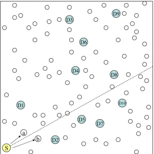
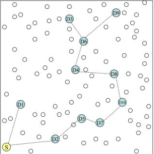
A sample run of LBM-D algorithm is given in Figures 3.1 and 3.2. A sam-ple topology with a source node and 10 destinations (D1,...,D10) is shown in Figure 3.1(i). The dashed lines originating from the source node (depicted as S) divide the region into subregions according to the alpha which is used to group the
CHAPTER 3. LOCATION BASED MULTICASTING ALGORITHMS 22
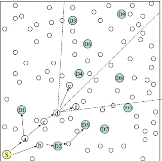
destinations. Solid arrows depict the transmission of multicast messages from one node to another. According to the case in Figure 3.1(i), destinations D1, D3, D4, D6, D8, D9 and D2, D5, D7, D10 reside in the same subregion. Therefore source node S makes two groups of destinations, (D1, D3, D4, D6, D8, D9) and (D2, D5, D7, D10). Figure 3.1(i) also shows the branching according to the groups that are created by the source node S. A multicast message with target destinations (D1, D3, D4, D6, D8, D9) is sent to node a and another multicast message is sent to node b with target destinations (D2, D5, D7, D10). In Figure 3.1(ii), node a decides to branch further with destination D1 and remaining destinations (D3, D4, D6, D8, D9) on the current branch. Destination D1 is reached and a multicast message with destinations (D3, D4, D6, D8, D9) is forwarded to the neighbor node c which is selected according to the neighbor selection algorithm described in Algorithm 3.6. On the other branch, node b forwards the message to D2 and destination D2 is reached. In Figure 3.2(iii), node d takes another branch with two groups of destinations (D3, D4, D6, D8, D9) and (D8). A multicast message with destinations (D3, D4, D6, D8, D9) is sent to node e and another multicast message with target destination D8 is sent to node f . Again nodes e and f are selected according to our neighbor selection scheme. On the other branch D5 is reached and removed from the destination list of the corresponding multicast message. Figure 3.2(iv) shows the final routes taken by the LBM-D algorithm in order to deliver the multicast messages to all destinations in the same manner explained above.
The weak point of the PBM algorithm was its neighbor selection strategy which requires 2n comparisons, where n is the number of neighbors of a node. This approach makes PBM unscalable, since in dense networks the number of comparisons will increase so rapidly, which will require excessive amount of en-ergy. However, in sensor networks power is a scarce resource which should be used very carefully. With LBM-D, we propose a neighbor selection algorithm whose running time is linear on the number of neighbors in the worst case. This feature of LBM-D makes it scalable and a better algorithm to be used for location based multicasting in wireless sensor networks.
S D1 D2 D5 D7 D8 D4 D6 D3 D9 a b D10 (i) S D1 D2 D5 D7 D10 D8 D4 D6 D3 D9 a b c (ii)
CHAPTER 3. LOCATION BASED MULTICASTING ALGORITHMS 24 S D1 D2 D5 D7 D10 D8 D4 D6 D3 D9 a c b d e f (iii) S D1 D2 D5 D7 D10 D8 D4 D6 D3 D9 a c b d e f (iv)
3.4
Our Proposed Algorithm II: Location Based
Multicasting with Direction According to
MST (LBM-MST)
Algorithms described in previous sections use only local information and depend-ing on this information make greedy decisions to deliver the multicast messages to destinations. LBM-D introduced a new scalable neighbor selection approach which makes it more scalable than PBM. LBM-MST is another algorithm that we propose which is based on LBM-D. LBM-MST is also a distributed algorithm, but it also uses the location information of the destinations in a global way and routes the multicast messages according to a minimum spanning tree which is calculated at the source node. Before starting to route packets, locations of all destinations are known to the source node. LBM-MST makes use of this information by calculating an Euclidean minimum spanning tree of all destinations. The infor-mation about the constructed MST is also forwarded with multicast messages, so that MST is only calculated once at the originator. The additional space over-head posed by MST in a packet is just a pointer to another destination, which determines the parent-child relationship between destinations. Furthermore, at branching points, destinations that a message carry is divided into pieces, so the size of multicast messages do not notably increase for LBM-MST. The analysis of the message overhead caused by extra pointers is given in Section 4.3.4.
Basically, LBM-MST draws a routing path for LBM-D by pointing to the destination which the multicast message should be delivered next. The path between two destinations is found by LBM-D. In other words, LBM-MST acts as a driver for LBM-D. Outline of LBM-MST is given in Algorithm 3.7.
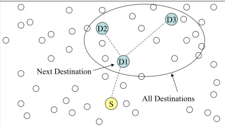
A multicast message in LBM-MST has both next destinations and all destina-tions. Next destinations are the immediate child nodes of the previous destination in the minimum spanning tree. All destinations are the nodes of the tree which is rooted at the previous destination according to MST. In Figure 3.3, for a multi-cast message that is sent from node S to D1, destination D1 is the next destination
CHAPTER 3. LOCATION BASED MULTICASTING ALGORITHMS 26
1: for all received message M do
2: if Msignature exists in Sent Message Signatures cache then
3: if there exists a neighbor n with an empty SMS cache then
4: Forward M to n
5: else
6: Drop message M
7: Continue for the next message
8: end if
9: end if
10: if MnextDestinations contains this then
11: Remove this from MnextDestinations
12: end if
13: if MallDestinations contains this then
14: Remove this from MallDestinations
15: MnextDestinations← GetImmediateChildren(MallDestinations)
16: end if
17: node group list ← GroupDestinations(MnextDestinations)
18: for all entry e in node group list do
19: nextN ode ← SelectNextNeighbor(e)
20: newM essage ← Create a message for e
21: Add Msignature into Sent Message Signatures cache
22: Forward newM essage to nextN ode
23: end for
24: end for
S D1
D2 D3
Next Destination
All Destinations
Figure 3.3: Next Destination and All Destinations. where all destinations are D1, D2 and D3.
Before starting routing a multicast message, the source (e.g. base station) cal-culates the Euclidean MST using the locations of all destinations by using Prim’s algorithm [15]. This information is hold in MallDestinations. Then next
destina-tions MnextDestinations are calculated by the procedure GetImmediateChildren.
The first message is forwarded to next destinations with LBM-D. MnextDestinations
are checked to see if the current node is one of the next destinations. If so it is removed from the list of next destinations and also from all destinations. Af-ter these operations, next destinations are calculated by GetImmediateChildren procedure for the current node. Having found the next destinations, they are grouped by the procedure GroupDestinations and multicast message for each group is forwarded to next neighbors as in the same way with LBM-D. The only difference with LBM-D is that in LBM-MST we group only the next destinations instead of all destinations. By this way we try to follow the paths drawn by the overall Euclidean MST constructed at the originator node.
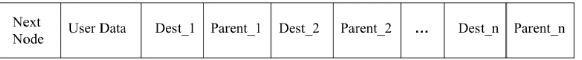
The procedure GetImmediateChildren is a simple routine which traverses the list of all destinations and finds the immediate child nodes of the current node. As we mentioned before, multicast messages carry the MST information in MallDestinations. This is achieved by holding a reference to the parent node of each
CHAPTER 3. LOCATION BASED MULTICASTING ALGORITHMS 28
are pointers for the parent nodes of the corresponding destination nodes depicted as Dest n. So if a destination’s parent is the current node, we add it to the list of immediate children childrenList. This list is returned by the procedure when it is done.
Next
Node User Data Dest_1 Parent_1 Dest_2 Parent_2 … Dest_n Parent_n
Figure 3.4: Multicast message used by LBM-MST.
1: childrenList ← Create an empty node list
2: for all node destination in allDestinations do
3: if destinationP arent = this then
4: Add destination to childrenList
5: end if
6: end for
7: return childrenList
Algorithm 3.8: Finding Immediate Child Nodes in LBM-MST.
A sample run of LBM-MST algorithm is given in Figure 3.5. The topology of the network, which is the same with in Figure 3.1, is shown in Figure 3.5(i). The dashed lines in Figure 3.5(i) shows the Euclidean minimum spanning tree of 10 destinations. The solid arrows in Figure 3.5(ii) depict the actual paths followed by the LBM-MST algorithm. As seen from the Figure 3.5(ii), LBM-MST tries to follow the Euclidean MST to minimize the number of total transmissions. In this sample case, LBM-D makes 15 transmissions to deliver the multicast message to all destinations, whereas LBM-MST requires only 20.
By following a minimum spanning tree of the destinations, we expect that LBM-MST will require less transmissions than LBM-D and PBM in order to deliver a message to all destinations. Since transmission is the most power con-suming operation for sensor nodes, we expect LBM-MST will use less power than LBM-D and PBM. Therefore, sensor nodes in LBM-MST will die later which prolongs the network lifetime. However, we should expect a greater average end-to-end delay for LBM-MST, because messages are enforced to follow the branches
S D1 D2 D5 D7 D10 D8 D4 D6 D3 D9 (i) S D1 D2 D5 D7 D10 D8 D4 D6 D3 D9 (ii)
CHAPTER 3. LOCATION BASED MULTICASTING ALGORITHMS 30
of a tree instead of following a direct path. But for most of the sensor network applications, network lifetime is the prominent concern and end-to-end delay has a little importance compared to energy conservation.
Evaluation
In this chapter we report the results of the experiments done to evaluate our algorithms. We evaluate our algorithms by comparing them with PBM [12] algorithm and also with each other. In order to achieve this, we implemented a basic wireless sensor network simulator. On this simulator we implemented the PBM routing algorithm and our routing algorithms. Hundreds of sample runs show that our algorithms work as expected and they are feasible to be used as location based routing protocols in wireless sensor networks. Before presenting the experiment results, we first describe the simulator that we have developed.
4.1
Simulator
Simulation is a very powerful method to evaluate a new routing algorithm which is especially designed for wireless sensor networks. Preparing a real testbed would be very costly and time consuming since the number of sensor nodes are too large and repeating the experiments for many times is not feasible. Additionally, we do not define a complete protocol suite which can be deployed on real sensor nodes, but we offer algorithms that can be used in routing protocols. Therefore we preferred simulation rather than using a real testbed.
CHAPTER 4. EVALUATION 32
After having decided using simulation to evaluate our multicast routing algo-rithms, we had to make another decision on whether we should use an existing simulator or implement our own simulator. Implementing a new simulator is not an easy task; however, if the complexity of the simulator is well adjusted, it can be more useful than the existing ones. In addition, most of the existing network simulators do not support wireless sensor networks. Another good reason to write our own simulator is to avoid unnecessary details which are nothing to do with our work. We think that it is better to construct a strong theoretical base before going into the protocol details which are related to the deployment issues. Our aim was to see if the algorithms we offer are good enough to be used as the core part of a location based routing protocol for wireless sensor networks.
Another important issue is the visualization of the process that is going on during the routing in the network. It makes easier to analyze the behavior of the algorithms and to see the weaknesses. So we wanted to see all the paths that are constructed by the routing algorithms on the graph of sensor nodes.
Based on the reasons mentioned above we decided to implement a basic wire-less sensor network simulator which is capable of performing the following tasks:
• Generating randomly distributed sensor network topologies,
• Running algorithms on densely deployed networks with high number of sensors,
• Repeating the experiments many times on different randomly generated topologies,
• Visually showing the constructed paths on the network,
• Generating customizable results beside the success ratio, number of total transmissions and end-to-end average delay.
We implemented our simulator with C# language on .NET environment. It has also a graphical user interface which enables defining input parameters easily
for single sample runs. We can immediately see the output of the algorithm on the sensor network graph. For long runs we prefer writing code blocks in which the input parameters can be easily substituted. Numerical results are written on the formatted files which are used for generating graphical charts.
The general approach that we follow for evaluating our algorithms is summa-rized in Figure 4.1.
1: for all Simulation Scenarios S do
2: for all Routing algorithms A (PBM, LBM-D, LBM-MST) do
3: for seed = 1 to n do
4: Generate random network topology T using seed
5: Run experiment with A for S on T
6: Store the output in a table
7: end for
8: Calculate the average values of the stored result
9: Write the average values into the output file
10: end for
11: end for
Algorithm 4.1: Simulation Approach.
This approach ensures that each algorithm is run on the same random topolo-gies, so it prevents any biased results that may occur due to the specific topology of the network generated.
As summarized in Figure 4.1, for each scenario we run PBM, LBM-D and LBM-MST algorithms with different seeds, and for each experiment we output the results, namely success rate, number of total transmissions, end-to-end delay and traffic overhead, and for each algorithm we calculate the average values for these metrics.
4.2
Scenarios
We evaluated our algorithms by comparing with a similar location based multicast routing algorithm PBM [12]. For all scenarios, each algorithm is run with same set of parameters. For an iteration of an experiment, all three algorithms are run
CHAPTER 4. EVALUATION 34
on the same network topology and with same destinations.
In order to generate the same network topologies for all algorithms, we used a fixed random seed for all algorithms, but at each iteration this random seed is changed to obtain unbiased results.
We focus mainly on the following metrics to evaluate our algorithms:
• Success Rate: We calculate success rate as the ratio of number of destina-tions that received the message divided by the total number of reachable destinations. In order to calculate a more reliable success ratio, it is neces-sary to omit the unreachable destinations due to topology of the network. Success rate is one of the most important metrics which shows how well the algorithms perform.
• Average End-to-end Delay: The timespan that begins with the transmission of a message from sink and ends with the reception of the message by a destination is called end-to-end delay. Average end-to-end delay is the average of all end-to-end delays that occur for each destination. We do not calculate end-to-end delay in time units, instead we measure the end-to-end delay by the number of hops taken from the sink to a destination. We use this metric only to compare the algorithms. We do not calculate absolute end-to-end delays, since it is dependent to the hardware used on the sensors. We also neglect the time spent for processing in the sensors.
• Number of Total Transmissions: Assuming each message hopping takes one transmission, we count the total number of transmissions made in order to the deliver the message from sink to all destinations. This metric is an indicator for the total power consumption due to transmissions and hence important for sensor network routing algorithms.
• Traffic Overhead: We also measure the total bytes transmitted during all transmissions which plays an important role on total power consumption. For each scenario we randomly deployed a set of sensor nodes on a 300x300 m area with a base station at the center. We take the transmission range of
the sensor nodes as 35 m. By changing the number of sensors deployed and the number of destinations we created many different test cases. For each scenario, we repeated the experiment many times to obtain reliable results. The destinations are randomly chosen from the deployed sensors in each scenario.
Without loss of generality, in our experiments we assume that we know the locations of the destination nodes. Indeed, in real applications we usually do not know the exact locations of any sensor in the region. Instead of sending messages to sensors, we send the messages to the regions or locations where we hope there exists some sensor nodes in those locations. This difference with real life and our simulation setup does not affect the general behavior of our algorithms. The only difference is we are sure that there exist a sensor node where we send the message in our simulations. To keep things simple, we just omit the regions and we directly send the messages to sensors whose locations are known. This approach can easily be applied to real life case by using a simple function that decides whether a sensor is inside the region that we want to send our message.
In all of our scenarios, we are given a set of destination nodes whose loca-tions are known and we try to deliver the message to all destinaloca-tions, which is transmitted by the base station located in the center of the network.
We created three kind of simulation scenarios:
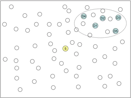
1. All destination nodes are located in the same region: In this scenario, all destinations are in the same subregion of the network. In other words, all destinations are located close to each other, thus constituting a destination region. We choose a fixed subregion to locate all destinations for each run to be able to see the difference of the algorithms clearer while changing the network topology in each time. A sample deployment for this scenario is shown in Figure 4.1.
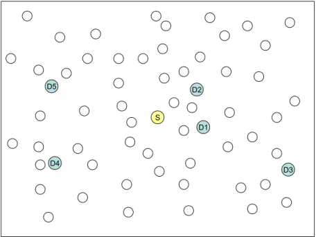
2. Destinations are located in separated regions: In this scenario, destinations are partitioned into groups and these groups are located in separate subre-gions of the network. In our simulations we tried to locate the destinations almost at the same locations to see the difference of the algorithms for each
CHAPTER 4. EVALUATION 36 S D2 D1 D4 D5 D3
run, while changing the topology each time. A sample deployment for this scenario is shown in Figure 4.2.
S D2 D1 D4 D5 D3
Figure 4.2: Destinations distributed separately.
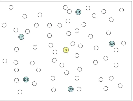
3. Destinations are located randomly: In this scenario, all destinations are located randomly in the network. A sample deployment for this scenario is shown in Figure 4.3.
While creating these scenarios we keep in mind the real life cases where we might want to send a message to a single region or several different regions. We also add the random case to be able to see the general behavior of the algorithms. In our simulations, we do not guarantee the connectivity of the generated network graph, but while calculating the success rate we omit the unreachable destinations in order to make the results more accurate.
CHAPTER 4. EVALUATION 38 S D2 D1 D4 D5 D3
4.3
Results
4.3.1
Success Rate
In this section we report simulation results which show the success rate of the algorithms for three different type of scenarios.
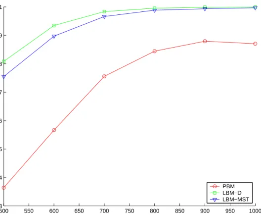
In Figure 4.4 success rates for randomly located destinations for all three al-gorithms are shown. As seen in Figure 4.4, both LBM-D and LBM-MST perform much better than PBM. Success rates for LBM-D and LBM-MST are close to each other, and while the network is getting denser, they reach success rates close to 1. An important point is that for sparse networks success rate of PBM is very low compared to LBM-D and LBM-MST. In addition, it appears LBM-D performs slightly better than LBM-MST for randomly deployed networks.
500 550 600 650 700 750 800 850 900 950 1000 0.3 0.4 0.5 0.6 0.7 0.8 0.9 1 #Sensors Success ratio PBM LBM−D LBM−MST
CHAPTER 4. EVALUATION 40
Figure 4.5 shows the success rates of the algorithms for randomly located destinations close to each other, in other words for destinations located in the same subregion. Our first observation is that, generally for destinations in the same region, results are better than the case where destinations are randomly distributed. Especially for sparse networks this observation holds. In this case, we see that PBM performs slightly better than LBM-MST. LBM-MST performs better than LBM-D for sparser networks. However, while the networks get denser, LBM-D starts to perform better than LBM-MST and reaches to the success rate of PBM. For networks with number of sensors is greater than 700, all three algorithms achieve high success rates which are very close to 1. A slight decrease can be observed for LBM-MST after 900 sensors.
500 550 600 650 700 750 800 850 900 950 1000 0.7 0.75 0.8 0.85 0.9 0.95 1 #Sensors Success ratio PBM LBM−D LBM−MST
Figure 4.5: Success rates for destinations grouped together.
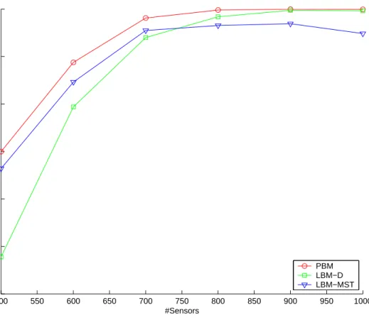
Success rates of the algorithms for randomly deployed destinations to sepa-rated subregions are shown in Figure 4.9. PBM and LBM-D perform better than the LBM-MST, especially for sparse networks that have less than 800 nodes. The
main reason of low success rate of LBM-MST for sparse networks is its inability of reaching child nodes of a node when unable to reach the node itself. However, in denser network environments, the probability of not reaching a node is low, so LBM-MST performs as well as PBM and LBM-D. We can observe that PBM and LBM-D achieve success rates very close to each other.
500 550 600 650 700 750 800 850 900 950 1000 0.3 0.4 0.5 0.6 0.7 0.8 0.9 1 #Sensors Success ratio PBM LBM−D LBM−MST
Figure 4.6: Success rates for separately distributed destinations.
4.3.2
End-to-End Delay
In this section we report simulation results for average end-to-end delay that is the time past from the transmission of a message from the sink until the reception by a destination node. As mentioned earlier, we give the end-to-end delays in terms of number of hops. Therefore, we omit the processing time that is spent in sensor nodes during the routing. Indeed this approach favors the PBM, because it spends much more time for message processing than LBM-D or LBM-MST. For
CHAPTER 4. EVALUATION 42
all scenarios, we can say that actually PBM performs worse than the reported results, but to calculate this difference we need parameters related to deployment and it is out of scope of this thesis.
Results of experiments for average end-to-end delay for randomly located destinations are shown in Figure 4.7. We observe that PBM and LBM-MST yield high average end-to-end delays than the LBM-D. We can also say that average end-to-end delays for PBM and LBM-MST are not directly affected with the increasing number of sensors deployed. They follow a path which is close to a straight line. High end-to-end delays occur in PBM and LBM-MST, because they tend to branch later than LBM-D. Especially for LBM-MST, messages have traverse the minimum spanning tree to reach the destinations which increases the end-to-end delays. Figure 4.7 also shows that average end-to-end delay for LBM-D decreases while the number of sensors increases.
500 550 600 650 700 750 800 850 900 950 1000 8 9 10 11 12 13 14 15 16 #Sensors Delay PBM LBM−D LBM−MST
Figure 4.7: Average end-to-end delay for randomly located destinations. Figure 4.8 shows the average end-to-end delays of the algorithms for randomly
located destinations that are close to each other. In this case, again PBM and LBM-D performs better than LBM-MST for the same reasons mentioned before. For all three algorithms, average end-to-end delays decrease while the networks get denser. 500 550 600 650 700 750 800 850 900 950 1000 11 12 13 14 15 16 17 18 19 20 #Sensors Delay PBM LBM−D LBM−MST
Figure 4.8: Average end-to-end delay for destinations grouped together. In Figure 4.9, simulation results showing average end-to-end delay for ran-domly located destinations into separated regions are given. LBM-MST results with higher to-end delays than PBM and LBM-D as expected. Average end-to-end delay for three algorithms do not change much with the number of sensors deployed but a very slight decrease can be observed while the networks get denser.
4.3.3
Number of Total Transmissions
In this section we compare the power consumptions of the algorithms in terms of total number of transmissions when a multicast message is delivered to all
CHAPTER 4. EVALUATION 44 600 650 700 750 800 850 900 950 1000 0 5 10 15 20 25 30 35 40 #Sensors Delay PBM LBM−D LBM−MST