Anil AlAn, YildirAY Yildiz, and Umit PoYrAz
High-Performance
Adaptive Pressure
Control in the Presence
of Time Delays
Digital Object Identifier 10.1109/MCS.2018.2851009 Date of publication: 18 September 2018
Pressure Control for use in
Variable-thrust roCket DeVeloPment
S
mart defense systems using missiles that can fine-tune their velocity profiles have significant technological superiority over their conventional counterparts. This tuning is possible, in part, due to the deployment of advanced sensing, actuation, and computation capabilities and sophisticated guidance, navigation, and control algorithms. The capability to alter velocity during operation helps sustain optimum perfor-mance for different flight conditions. In addition, it makes it possible to slow down while turning and then speed up along a straight path, rendering the maneuvers more effi-cient. This ability to modify velocity (known as throttle-ability) is also known to increase a missile’s no-escape zone, which is the maximum range that the missile can out-run its target [1]. As presented in “Summary,” this article discusses the advanced control technologies needed to ob-tain throttleability.To achieve throttleability, it is important to understand the underlying dynamics leading to jet-engine propul-sion. Propulsion systems in jet engines generate thrust via a burning process that creates a chemical reaction between fuel and an oxidizer. These systems can be divided into two groups in terms of the source of the oxidizer: air-breathing jet engines (which get the oxidizer from the surrounding atmosphere) and non-air-breathing jet engines (which carry the oxidizer along with the fuel, making them closed sys-tems). Conventional solid-rocket engines, which carry their fuel and oxidizer in a solid state, are examples of non-air-breathing jet engines. They are relatively easy to manufac-ture (since they do not contain complex moving parts) and produce standard thrust performance over a variety of flight conditions (since they are closed to their environments). Besides the advantage of simplicity, the thrust can also be controlled, which makes them variable-thrust solid propul-sion systems [2]. However, the specific impulse values (the total impulse that a rocket engine can produce per unit of propellant burnt) is very low compared to air-breathing engine systems since it must also carry the oxidizers. As such, conventional solid-rocket engines are less preferable for long-range cruise flights. Air-breathing jet engines, on the other hand, compress the air during operation using various methods (such as ramjets, scramjets, turbojets, and turbofans) and mix it with the fuel for the combustion and to yield thrust.
ThROTTLEAbLE DuCTED ROCkETS
A ramjet is an air-breathing jet engine that utilizes forward motion to collect and compress air using air-intake open-ings. Ducted rockets are ramjet-type engines (see Figure 1). The air then moves to the ram combustor, where it is mixed with the oxidizer-deficient gaseous fuel provided by the gas generator (GG).
The GG uses a preburn process to produce the gas-eous fuel from the solid propellant. The fuel is then sent to the ram combustor through a connection between the
GG and the ram combustor by a pressure gradient. The appeal of the ducted rockets is the possibility to control the fuel flow rate (supplied by the GG) into the ram combustor, which transforms these rockets into throttleable ducted rockets (TDR). TDRs, therefore, combine the advantages of different propulsion systems: high specific impulse values of air-breathing engines; simplicity of solid rocket engines; and throttleability, which is available in liquid fuel ramjet engines, for example. Although the specific impulse values in TDRs are high, metallic particles (boron or aluminum) are typically placed inside the solid propellant to further enhance it [3], [4]. These particles are not burnt during the initial burning process at the GG and sent to the ram com-bustor with the gaseous fuel.
Summary
T
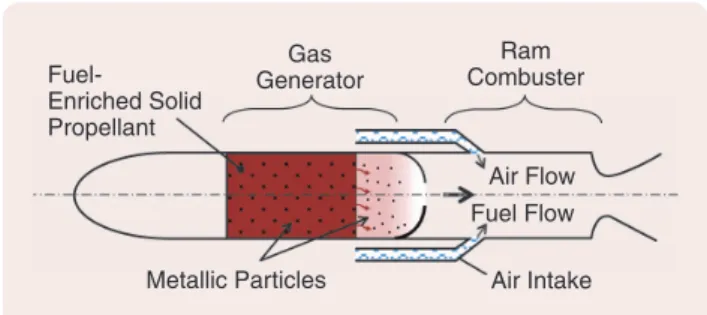
he focus of this article is the pressure-control problem of gas generators employed in variable-speed rockets. the ability to change the speed during operation enables these rockets to adjust to the demands of different types of maneuvers and varying flight conditions. As a result, speed-controllable rockets provide a dramatic advantage over their alternatives with fixed speed profiles. in throttle-able ducted rockets, speed variation is achieved by chang-ing the fuel flow rate (throttleability), which requires a care-ful controller design. the article provides a detailed review of the current state of rocket propulsion control and the main challenges in the field. A controller (which contains a unique combination of traits such as fast adaptation, delay compensation, and provision of a smooth response) is in-troduced as a solution to the pressure control problem in air-breathing rocket propulsion. the superior performance of the controller, compared to existing alternatives, is dem-onstrated through experimental tests, using a test setup pro-vided by roketsan, inc.figure 1 throttleable ducted rocket (tDr) components. tDr
pro-pulsion systems contain two main parts, the gas generator (GG) and the ram combuster (rc). Fuel-rich (or oxidizer-deficient) solid propellant in the GG is ignited and partially burned to obtain fuel in the gaseous form, which is then sent to the rc to combine with air received and compressed by the air intakes for further combustion to produce thrust. Air Intake Fuel-Enriched Solid Propellant Metallic Particles Gas Generator Ram Combuster Fuel Flow Air Flow . . . . . . . . . . . . . . . . . .
Alternative Methods of Obtaining
the Variable Fuel Flow Rate
In TDRs, the flow rate of the gaseous fuel that is generated determines the amount of thrust. Various methods are used to obtain a variable fuel rate [5], [6], which are listed below and depicted in Figure 2.
» Changing the burning area of the propellant in the GG in a controlled manner: Assuming that the solid propellant burns within a uniform cross-sectional area (known as “cigarette-type burning”), such as in Figure 2(a), their solid grains can be trimmed to have different cross-sectional areas at each moment of burn. A smaller burning area generates less fuel and, therefore, less thrust. However, once a trimmed propellant is ignited, it is impossible to make any changes to its geometric structure during operation. Therefore, solid rocket engines with trimmed propellants have prescribed thrust profiles over all operating regions.
» Introducing secondary injection to the GG chamber to con-trol the burning rate: It is known that the burning rate of a solid propellant is affected by the pressure of the chamber, where the relationship is determined by the pressure sensitivity of the propellant [7]. There-fore, the burning rate of the solid propellant can be controlled by controlling the pressure at the GG chamber. One way to achieve this is by introducing a secondary medium. However, this method requires complex parts, such as a secondary chamber.
» Utilizing a vortex valve that introduces a swirl to the flow to control the effective throat area: The injected fuel flow rate from the GG to the ram combustor depends on the effective throat area between the two parts.
There-fore, changing the effective throat area can be counted as a method for manipulating the fuel flow rate. A vortex valve can induce a swirling flow at the throat to increase the flow resistance (or reduce the effec-tive throat area) at the expense of increasing the system complexity.
» Changing the throat area between the GG and the ram com-bustor using a control valve: The effective throat area can be varied using a control valve, which is less com-plex than the vortex valve. Among the listed methods here, this method is used the most often ([5], [8]–[11]), and the control approaches discussed in this article assume the control valve is the actuator.
Control Solutions to Obtain Variable Speed or Thrust
There are two control solutions for the speed or thrust con-trol problem of TDRs. The first solution forms a single-loop controller structure, where the controller calculates the necessary throat area between the GG and the ram combustor to track a given speed or thrust reference [8]– [12]. The block diagram for this solution is provided in Figure 3(a). The second solution creates a hierarchical control structure, where an outer-loop speed/thrust con-troller calculates the required GG pressure to obtain a desired speed or thrust profile, which is then used as a reference for the inner pressure control loohp, as shown in Figure 3(b), [1], [13]–[15].
These two control solutions have distinct advantages over each other. The single-loop solution is simpler to design. However, the hierarchical control structure is safer, due to gas pressure stability; it is easier to keep the pressure inside the GG within safe limits by utilizing a separate
figure 2 Methods of regulating the fuel flow rate from the gas generator to ram combustor (figures originated from [5] and [6], used with
permission): (a) changing the burning area of the propellant, (b) using secondary injection, (c) using a vortex valve, and (d) using a
con-trol valve.
Air Intake Solid Propellant
with Tapered Grain Gas Generator
Ram Combuster
Ram Combuster
Fuel Flow Fuel Flow
Air Intake Solid Propellant Gas Generator Secondary Injection Media Control Valve Air Intake Solid Propellant Gas Generator Ram Combuster Fuel Flow Swirling Flow Air Intake Solid Propellant Gas Generator
Ram Combuster Fuel Flow Control Valve Flow Diverter (a) (b) (c) (d) Injection of Control Flow
pressure controller, which prevents undesired pressure buildup and possible structural damage. The GG pressure control loop in the second method is the focus of this article. It is shown here that seemingly separate tools, such as delay compensation, adaptation to uncertainties, and transient response improve-ment, can be combined to obtain solutions that can dramati-cally improve the performance of a challenging control loop, such as pressure control, over conventional approaches. Note that the nonminimum phase dynamics between the throat area and the fuel mass flow rate does not effect the inner pressure control loop and should be handled in the outer speed or thrust loop. This nonminimum phase dynamics is explained further in “Nonminimum Phase Behavior of Thrust in Throttleable Ducted Rockets.”
The discussion in this article on the employment of advanced control methodologies should benefit practitioners whose goal is to obtain a fast system response in safety-critical applica-tions where nonlinear dynamics, time-varying parame-ters, and time delays pose significant challenges. One of the most common approaches to control GG pressure is uti-lizing linear controllers that are designed based on a model
of the system obtained by linearizing the nonlinear dynam-ics around a certain operating point [14], [16], [17]. Although this method is simple to implement, it may limit the per-formance when the operating point changes, as shown in the simulations and experimental studies presented in this article. Apart from the nonlinearities, another challenge for GG pressure control is that as the fuel burns, the free volume inside the GG increases with time, which makes the system time varying. Moreover, the GG dynamics contain several uncertainties emanating from metallic particles inside the solid fuel, such as deposition at the nozzle throat and abla-tion of mechanical elements. One of the more sophisticated control approaches to address these issues is gain schedul-ing [13], [15], where full knowledge of the controlled plant in the form of a high-fidelity mathematical model is employed to prepare lookup tables that are then used to assign appro-priate controller gains at different operation modes and conditions. Another method, which is employed for the flight-performance evaluation study of the Meteor mis-sile, is the performance funnel approach [18], [19], where a proportional controller is utilized with a time-varying gain
figure 3 Alternative speed control loops of a throttleable ducted rocket. (a) the single speed or thrust loop, formed with the speed or
thrust controller, that calculates the necessary throat area directly to set the missile speed equal to the desired speed, fuel flow regula-tion from the gas generator (GG) to the ram combuster, and combuster and missile dynamics. (b) the speed or thrust control loop hierarchical structure. the GG loop serves as an inner loop in this structure and is responsible for providing the required gas pressure inside (GG) that is dictated by the speed or thrust controller. the GG loop contains the pressure controller, actuator, valve mechanism, and GG dynamics. the output of the GG loop is the mass flow rate of the fuel.
Desired Speed
Speed
Controller RegulationFuel Flow RAM Combuster andMissile Dynamics Fuel Flow to
RAM Combuster Required
Throat Area
Missile Speed
RAM Combuster and Missile Dynamics Desired
Speed/Thrust
Measured Speed/Thrust
Speed/Thrust Controller Required Pressure Gas Generator Loop
Fuel Flow to RAM Combuster Required Pressure Pressure
Controller
Required
Throat Area ThroatArea Gas
Generator Dynamics Measured Pressure Fuel Flow to RAM Combuster Actuator and Valve Control Mechanism (a) (b)
that is adjusted online to keep the error of the closed-loop system within a predefined performance funnel. One practi-cal disadvantage of funnel control is that, although the error stays inside a funnel, it does not guarantee the convergence to zero [20], which reduces the steady-state performance of the closed-loop system.
The final challenge considered in this article for gas pres-sure control is the time delay originating from prespres-sure measurement, computational, and actuation delays and those inherent in system dynamics. The Smith predictor [21] is an early approach to addressing the time delay in control problems, where future prediction of the system output is
used in the feedback that mitigates the destabilizing effects of the delay. The finite spectrum assignment method [22] and adaptive delay compensation tools are also developed [23]–[25]. Other notable studies on the adaptive control of time-delay systems are shown in [26] and [27], where unknown input delays and both state and input delays are addressed, respectively. Adaptive-loop recovery [28] is also shown to work well with the time delays of the flight-control problem. In addition, the extension of predictor feedback to nonlinear and delay-adaptive systems with actuator dynamics mod-eled by partial differential equations is discussed in [29]. A Pade-approximation-based approach for addressing the
Nonminimum Phase Behavior of Thrust in Throttleable Ducted Rockets
W
hen represented in the Laplace domain, a nonminimum phase system transfer function has unstable zeros, which means that at least one root of the numerator polynomial in the transfer function has positive real parts. Nonminimum phase be-havior in the time domain manifests itself in the step response, where the response initially moves to the “wrong” direction be-fore it eventually reverses direction and approaches its steady-state value.in throttleable ducted rockets (tDrs), the relationship be-tween the throat area and the fuel mass flow rate shows a non-minimum phase behavior. this does not affect the gas gen-erator (GG) pressure control since, in the pressure loop, the feedback variable is the pressure inside the GG (see Figure 3). therefore, this phenomenon should be addressed in the outer speed or thrust loop.
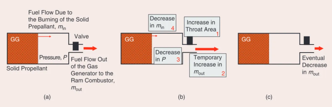
the dynamics of the nonminimum phase behavior in tDrs is demonstrated in Figure S1. consider the case when the fuel flow rate generated inside the GG is equal to the ejected fuel flow
rate. When there is a step increase in the throat area, it causes an instant discharge of the fuel, which increases the ejected mass flow rate instantly but decreases the pressure inside the medium. the burning rate of the solid propellant decreases due to its pressure sensitivity (it is known that the burning rate is af-fected by the pressure of the chamber [7], which is the pressure sensitivity of the propellant). this pressure sensitivity reduces the pressure to a lesser value. the mass flow rate coming out of the GG (assuming chocked flow conditions at the throat) is
, m c PA out= )t o (S1)
where At is the throat area, P is the pressure, and c* is the
characteristic velocity of the fluid inside the GG. therefore, the flow rate out of the GG eventually decreases. A step increase in the throat area initially increases but eventually decreases the mass flow rate of the ejected fuel, which indicates a non-minimum phase behavior.
figure s1 the nonminimum phase behavior of ejected fuel from the gas generator (GG). (a) shows the steady-state conditions.
in (b), a positive step change in the throat area is given as an input to the system, which results in a temporary increase in the ejected mass flow rate and a decrease in the pressure inside the GG. the burning rate of the solid propellant decreases due to the decrease in pressure. in (c), after the transients are removed, the ejected mass fuel flow rate moout reaches its reduced
steady-state value due to lower burning rates. Hence, a step increase in the throat area initially increases the ejected flow rate, but then the flow rate eventually decreases, which is a nonminimum phase behavior.
GG
Fuel Flow Due to the Burning of the Solid Prepallant, min
Pressure, P Fuel Flow Out of the Gas Generator to the Ram Combustor, mout Increase in Throat Area Decrease in P Temporary Increase in mout GG Decrease in min 1 2 4 3 GG Eventual Decrease in mout Solid Propellant Valve (a) (b) (c)
time delay in actuators in the context of model reference adaptive control (MRAC) theory is addressed in [30] and [31]. It is shown that by reinforcing classical ideas from adaptive control literature with recent developments in delay com-pensation and transient performance improvement, the pre-viously discussed control challenges can be addressed and a high-speed pressure response can be obtained in a safe manner by preventing excessive oscillations, without the need for precise system dynamics and the conservatism of robust approaches. Aside from pressure control problems, the benefits of combining delay compensation, adaptation, and transient response improvement methods can be real-ized in a variety of domains where uncertainties and time delays play a dominant role. Various adaptive delay com-pensation approaches have already been implemented in a wide array of plants, including teleoperation systems [32], internal combustion engines [33], [34], biology [35], [36], space systems [37], and transportation [38]. In this article, a unique combination of an adaptive delay compensation method [39] and adaptive transient performance improve-ment method [40]–[43] is discussed. The presented solution, termed the delay-resistant closed-loop reference model (DR-CRM) adaptive controller is investigated through simula-tions and experimental studies, where comparisons with progressively more sophisticated control approaches are carefully conducted.
In TDR research, cold-air test setup is widely considered the critical step in the validation of subsystems and meth-ods. The setup is used, for example, to validate the numerical simulation results of flow characteristics, test the structures that are used to change the throat area, and characterize the materials that are planned for use in the construction [44]– [49]. A control algorithm is also a subsystem that must be qualified. This test setup conducts a comparative analysis of alternative control systems [50], which is then used to acquire a proper control methodology based on the gained insight. For the purposes of this article, Roketsan, Inc. provided its facilities to create an industrial-grade test setup that was uti-lized for the experimental studies.
The following sections present the nonlinear model of the system used for the discussions on alternative control approaches. The first principles for obtaining the initial model and enhancements through the use of experimental data are explained in detail. Moreover, the theory behind the DR-CRM adaptive controller is presented. Background material on this topic is provided in “Classical Model Ref-erence Adaptive Control.” In addition to the fundamental theory, practical concerns (such as drifting of the control parameters due to the controller’s attempts to compensate for noise or unmodeled dynamics) and the determination of how fast to update the adaptive parameters are also dis-cussed. Simulation and experimental implementation of the proposed control approach is presented. Depending on the mission, the desired pressure variations in TDRs can be small or large around several different operating regions. It
is demonstrated that the investigated control solution pre-vents excessive pressure oscillations without slowing down the response of the system in all of the operating regions and pressure variation amplitudes that are tested.
buILDING ThE NONLINEAR MODEL
ThROuGh FIRST PRINCIPLES AND DATA
Conducting experiments at high pressures is both danger-ous and expensive. Therefore, a high-fidelity plant model that can be used to test and tune alternative control ap -proaches in the simulation environment is invaluable for the industry. A realistic model not only helps to minimize controller tuning time and effort in the experimental stage but also provides valuable insights on creating safe test sce-narios (where the pressure is kept within allowable limits) that will protect the workers and system hardware. This section presents the procedures to obtain a reliable system model, which mainly consist of using the first principles to obtain an initial model and employing experimental data to improve model fidelity. A modeling procedure combin-ing the first principles and experimental data can produce a high-fidelity model that is beneficial for controller testing in the simulation environment. However, this model can be unnecessarily complicated for the controller development. As will be presented in the later parts of this section, basic model simplification methods can be implemented to obtain a model for controller development.
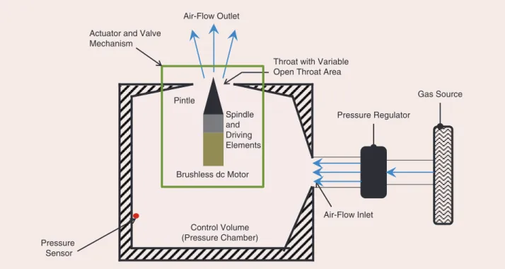
Cold-air test setup consists of a control volume (pressure chamber), actuator, valve mechanism, pressure sensor, drive-train elements, gas supply, and pressure regulator (see Figure 4). A continuous flow of gas is provided by a nitrogen source to the plant from the inlet, and the flow rate is adjusted by a pressure regulator. Besides its well-known characteris-tics, nitrogen is a safe (nonflammable at testing conditions and nontoxic) and inexpensive gas that can be easily obtained. The output of the model (which is the pressure inside the control volume) is controlled by changing the exit throat area of the flow. In the experimental setup in this article, the throat area is increased or decreased using the linear motion of a pintle, whose geometrical analysis is provided in this section. Another solution uses a piston-type valve. A comparative analysis of these two alternatives, together with a geometri-cal analysis of the latter, is provided in “Pintle Versus Piston.” Drivetrain elements convert the rotational motion of the actua-tor (a brushless dc moactua-tor) to translational motion of the pintle with the required amount of reduction.
Pressure Dynamics
Assuming ideal gas conditions, the difference between the mass flow rates going into the control volume (pres-sure chamber) moin [kg/s] and out of the control volume
moout [kg/s] is
,
Classical Model Reference Adaptive Control
M
odel reference adaptive control (MrAc) is commonly used for linear time-invariant systems with uncertain parameters. A brief introduction to this controller is provi-ded for both a scalar and higher-order input, single-output system.SCALAR CASE
consider a first-order plant
( ) ( ) ( ),
x to =ax t +bu t (S2) where x!0 is the output, u!0 is the input of the plant, and ,a b!0 are the plant parameters. in classical MrAc, the plant output is expected to track the output of a reference model (teacher). the closed-loop system specifications are enforced through this reference model. the reference model is defined as
( ) ( ) ( ),
x tom =a x tm m +b r tm (S3)
where x rm, !0 are the reference model output and a bounded command (reference) to the closed-loop system, respectively.
am and bm are the parameters that are chosen to specify the
closed-loop system requirements. For this scalar case, it is sufficient to choose am1 to satisfy the necessary stability 0 conditions for both the reference model and the overall closed-loop system. However, additional requirements must be
satis-fied for the higher-order case, which are explained in the sec-tion “Higher-order case.”
the control problem is to find the controller ( ) ( ) ( ),
u t =ix t +kr t (S4) such that with the controller parameters ,ik!0, the tracking error e t1( )=x t( )-x tm( ) between the plant and the reference model outputs converges to zero. the control problem can eas-ily be solved if the plant parameters ,a b are known precisely.
if the controller parameters are chosen as * (a a b)/
m
i = - and
, /
k*=b bm then the closed-loop system dynamics become
the same as those of the reference model. the existences of these ideal control parameters are the matching conditions. However, it is not always possible to determine the exact val-ues of plant parameters , .a b in the design of MrAc, it is
as-sumed that the plant parameters (and hence the ideal values of the controller parameters, , )i*k* are unknown. therefore, the control parameters are adjusted online in a unique way (which is explained below) to make the tracking error reach zero and maintain all the system signal stability. controller parameter errors ( )iu t =i( )t -i* and ( )k tu =k t( )-k* are
de-fined as the deviations of the real parameters ( ), ( )i t k t from their ideal values. Substituting (S4) into (S2), the closed-loop system becomes
( ) ( ) ( ) ( ) ( ) ( ) ( ).
x to =a x tm +b r tm +b t x tiu +bk t r tu (S5)
figure s2 A model reference adaptive control (MrAc) structure, originated from [51]. controller parameters T( ),t T( ), ( ),t t
1 2 0
i i i and
( )
k t are updated online with the tracking error e t1( ) between the plant output and reference model outputs.
kmZm(s) Rm(s) kpZp(s) Rp(s) ym(t ) yp(t ) u (t ) r (t ) e1(t ) + – k + Σ + + + ω1(t ) ω2(t ) θ0 θ1T θ2T ∧, l ∧, l
to understand the error dynamics between the plant and refer-ence model outputs in the presrefer-ence of parameter errors, (S3) is subtracted from (S5) to obtain
( ) ( ) ( ) ( ) ( ) ( ).
e to1 =a e tm 1 +b t x tiu +bk t r tu (S6)
error dynamics can be analyzed using a Lyapunov function candidate ( , , ) ( ) ( ) , sgn sgn V e k e b b b b k 2 1 2 2 1 12 1 2 2 2 i c i c = + + u u u u (S7)
where sgn $ is the signum function and ,( ) c c1 2 are positive
constant scalars. Using the derivative of the Lyapunov function candidate and (S6) gives
( ) ( ) . sgn sgn V a e xe b b re kb bk m 12 1 1 1 2 c i i c = + + + + o e uo o u e uo o (S8)u
if the adaptation laws to update the controller parameters are chosen as ( ) ( ) ( ) ( ) ( ) ( ) ( ) ( ) ( ) ( ), sgn sgn t t b e t x t k t k t b e t r t 1 1 2 1 / / i i c c = = -uo o uo o (S9)
then Vo#0 and the boundedness of all signals in the system are ensured. Furthermore, since Vp=2a e em 1 1o is also bounded,
e1"0 as t " 3 from barbalat’s Lemma [S1].
hIGhER-ORDER CASE
consider the case of a single-input, single-output linear plant with a transfer function of order larger than one and a relative order equal to one.
Definition 1
A transfer function ( )G s is called a strictly positive real (SPr)
transfer function if it satisfies the following criteria:
• G(s) is stable.
• Re G i[ ( )]~ 20 for ~20. • G( )3 20.
Lemma 1 [51], [S1]
consider the dynamical system described by ( ) ( ) ( ) ( ), ( ) ( ), ( ) ( ), x t Ax t b t w t y t h x t z t ky t T T 1 z = + = = o (S10) where k is an unknown constant whose sign is known, the pair ( , )A b is stabilizable, ( , )h AT is detectable, and the transfer
function ( )H s =h sI AT( - )-1b is SPr. in addition, the scalar
( )
z t1 and vector ( )w t can be measured. Under these
condi-tions, if the adjustable parameter ( )zt is updated using the adaptive law
( )t sgn( ) ( ) ( ),k z t w t1
zo = - (S11)
then the equilibrium point x=0,z=0 is uniformly stable in the large. Furthermore, if ~ is bounded, then ( )x converges t
to zero asymptotically.
consider the plant dynamics described by the following state-space representation , , x A x b u y h x p p p p p Tp p = + = o (S12) where xp is an n-dimensional state vector, u is the scalar
con-trol input, and y is the scalar plant output. the matrix Ap and
vectors bp and hp are assumed to be unknown. the transfer
of this plant is ( ) ( ) ( ) ( ) ( ) . U s Y s k R sZ s h sI A b p p p p p T p 1 p = = - - (S13)
it is assumed that all of the roots of the numerator polynomial ( )
Z sp have negative real parts. this is required to prevent the
possibility of an unstable pole zero cancellation.
the state-space representation of the nth-order reference model is , x A x b r y h x m m m m m mT m = + = o (S14) with the associated transfer function
( ) ( )( ) ( )( ) ( ) . W sm Y sR sm k R smZ s h sI A b m m m T m 1 m / = = - - (S15)
equation (S15) of the reference model is selected to be SPr, and the need for this requirement will become apparent in the following. the gain km is assumed to be positive for simplicity.
the MrAc controller structure that makes the error e1=yp-ym
converge to zero is given in Figure S2. Using the variables in the figure, the equations describing the controller dynamics are
( ) ( ) ( ), ( ) ( ) ( ), ( ) [ ( ), ( ), ( ), ( )] , ( ) [ ( ), ( ), ( ), ( )] , ( ) ( ) ( ), t t lu t t t ly t t r t t y t t t k t t t t u t t t p T p T T T T T T 1 1 2 2 1 2 1 0 2 / / ~ ~ ~ ~ ~ ~ ~ i i i i i ~ K K = + = + = o o (S16) where K!0(n-1) (#n-1) is a matrix with eigenvalues that have
negative real parts and the pair ( , )lK is controllable.
the first step in designing the MrAc is to show the existence of a fixed (nonadaptive) controller that will ensure that the closed-loop transfer function becomes equal to the transfer function of the reference model. in this regard, assuming a fixed control pa-rameter gain vector ,if the following definitions can be made:
( ) ( ) ( ) , ( )( ) ( ) . s C s sI l D ss sI l f T f Tf 1 1 0 2 1 / / m i -K m i +i -K - - (S17)
Note that the degree of the polynomials ( ),ms ( ),C s and ( )D s
are (n-1), (n-2), and (n-1), respectively. Using (S17), the overall closed-loop transfer function (assuming fixed controller gains) is
where R [J/(kg-K)] is the specific gas constant and P [Pa], T [K], and V [m3] are the pressure, temperature, and volume of the gas inside the control volume. Assuming an isother-mal process with no change in the control volume, then
. Vo =To =0
The mass flow out of the control volume is a function of the throat area A mm^ t6 2@ and the pressure inside the con-h
trol volume (P). Assuming chocked flow conditions, the relationship between the throat area and resulting mass flow rate out of the control volume can be calculated as [13]
, m PA RT PAc 1 2 t 1 t out c c = + ) = ) c c -o ec mc mo (2)
where c is the specific heat ratio of air, T) is the
tempera-ture at the throat, and c) [m/s] is the characteristic velocity of the gas inside the control volume. Using (1) and (2) yields
, Po =c m1 oin-c PA2 t=M c PA- 2 t (3) where c1=(RT V c)/ , 2=c c1/ ,) and M=c m1 oin. ( ) ( )( ) ( ( ) ( )) ( )( ) ( ) ( ) ( ). W s Y sR sp s C s R sk k Z s k Z s D ss p p p f p p / m m = - - (S18)
ideal fixed control parameter values ,k* *T, *T,and *
1 2 0
i i i can be selected to make the closed-loop transfer function (S18) equal to the reference model transfer function (S15). Note that K can be selected such that ( )ms =Z sm( ) [see (S17)] . Also, ( )Cs can be shaped using i1f, and ( )D s can be shaped using i0f and
.
f
2
i therefore, there exist certain ideal values, , ,* * 1 2
i i and * 0
i
for these fixed parameters such that when *, *,
f f 1 1 2 2 i =i i =i and *, f 0 0 i =i both ( )ms -C s( )=Z sp( ) and ( )R sp -k D sp ( )=R sm( ) (S19) are satisfied. Finally, kf can be selected such that kf=k*=k km/ .p
it can then be verified that with these fixed values, the closed-loop transfer function (S18) becomes equal to the reference model transfer function (S15).
Having established the existence of the ideal control param-eters to make the closed-loop transfer function equal to the ref-erence model transfer function, the second step of the controller design can be introduced. However, note that the value of the ideal parameters are not known because plant parameters are unknown. even though the ideal parameters are unknown, it can be shown that, with certain online adaptation mechanisms, they can be adjusted in such a way that the tracking error approaches zero while keeping all system signals bounded. to demonstrate how this is achieved, the dynamics of the plant and controller are first rewritten using (S12) and (S16) as
( ) ( ) ( ( ) ( )), ( ) ( ) ( ( ) ( )), ( ) ( ) ( ( )). x t A x t b t t t t l t t t t l h x t p p p p T T p T p 1 1 2 2 i ~ ~ ~ i ~ ~ ~ K K = + = + = + o o o (S20)
Using the definitions ( )k t k t( ) k*, ( )t ( )t *,
1 1 1 / - i /i -i u u iu0( )t / ( )t *, ( )t * 0 0 2 2 2 i -i iu =i -i and ( )t [ ( ),k t T( ), ( ),t t 1 0 z = u iu iu ( )],T t 2 iu (S20) can be rewritten as [ ], , x A x b k r y h x * mn mn T p mnT z ~ = + + = o (S21) where x=[ ,xTp~ ~T1, T T2] and , , . A A b h l h lh b l b l b b l h h 0 0 0 0 * * * * * * mn p p pT p T p T p T T p T T mn p mn p 0 0 1 1 2 2 i i i i i i K K = + + = =
>
H
>
H
>
H
(S22) if the control parameters ( )i t become equal to their ideal val-ues ,i* then the closed-loop transfer function becomes equalto the reference model transfer function. therefore, using (S21) and the fact that the control parameter deviation vector
z becomes identically zero, the reference model can be rep-resented by , , x A x b k r y h x * mn mn mn mn m mnT mn = + = o (S23) where x [x* , * , * ]
mn= pT ~1T~2T. it is noted that xmn consists of
the ideal states in the reference model corresponding to the closed-loop system states x tp( ),~1( ),t and ~2( )t . the
refer-ence model transfer function (S15) is nth order and (S23) is (3n–2)th order. therefore, (S23) is a nonminimal state-space representation of the reference model. Defining the errors e/ -x xmn and e1/yp-ym and subtracting (S23)
from (S21) yields ( ) ( ) ( ) ( ), ( ) ( ). e t A e t b t t e t h e t mn mn T mn T 1 z ~ = + = o (S24) Lemma 1 illustrates that, if the controller parameters are ad-justed online by employing the following adaptation rules, then all of the system signals will be bounded and the tracking error
e1 will converge to zero
( ) ( ) ( ) ( ), ( ) ( ) ( ) ( ), ( ) ( ) ( ) ( ), ( ) ( ) ( ) ( ), sgn sgn sgn sgn k t k e t r t t k e t y t t k e t t t k e t t p k p p p p 1 0 0 1 1 1 1 1 2 2 1 2 c i c i c ~ i c ~ = = = = -o o o o (S25)
where , , ,c c ck 0 1 and c2 are positive constants that define the
speed of adaptation. these variables are also called adapta-tion rate parameters. A more detailed discussion and the ex-tension for more general classes of plants can be found in [51].
REFERENCE
[S1] J.-J. e. Slotine and W. Li, Applied Nonlinear Control. eagle Wood cliffs, NJ: Prentice-Hall, 1991.
figure 4 A schematic of the cold-air test setup. the overall cold-air test setup consists of a pressure chamber, an actuator, a valve mechanism, a pressure sensor, drivetrain elements, a gas supply, and a pressure regulator. A continuous stream of gas (supplied by the gas source and regulated by the pressure regulator) fills the pressure chamber, which has inlet and outlet ports. the control valve at the exit port is used to control the gas pressure inside the chamber.
Control Volume (Pressure Chamber)
Throat with Variable Open Throat Area Air-Flow Outlet Air-Flow Inlet Pressure Regulator Gas Source Pressure Sensor
Actuator and Valve Mechanism Spindle and Driving Elements Brushless dc Motor Pintle
Actuator Dynamics
In the experimental setup built by Roketsan, Inc., a brush-less dc motor is used as the actuator. The motor is run in position control mode, and an encoder is used to measure the position or speed of the rotor. A first-order dynamic is sufficient enough to model this architecture
( ) ( )( ) , Wacts tt s1 1 com mes act i i x = = + (4)
where imes [quadrature] is the measured actual rotational position of the rotor, icom [quadrature] is the commanded rotational position (4000 quadratures correspond to one rotation), and iact is the actuator closed-loop time constant.
Valve Geometry and Drivetrain Elements
The drivetrain elements consist of a gear box and a ball screw spindle to convert the rotational motion of the motor into the translational motion of a pintle at the throat area (see Figure 5). The linear position of the pintle determines the throat opening.
The pintle has one degree of freedom in the x-direction and open throat area changes as the pintle moves along the x-axis due to its conical surface. The cross-sectional area of the cylindrical part at the back of the pintle is smaller than the fixed throat area, which ensures that the open throat area At is always larger than zero and protects the system
from rapid pressure build up. The valve and the drive train models are explained next.
Valve Geometry
There exists a complex relationship between the movement of the pintle and the minimum throat area, where the choked flow conditions occur, due to their complex geom-etries [44], [46]. The size and location of the minimum throat area is hard to estimate analytically because that location of the choked flow line, where the throat area is minimum, shifts toward the upstream as the pintle moves into the throat [46]. The size of the open throat area can be approximated as the projection of the real area on the verti-cal surface that is perpendicular to the pintle center line. Movement of the pintle along the x-axis reduces the pro-jected throat area by
( ) , tan
y=y0- ax (5)
where y0 is the radius of the pintle at the cylindrical base and a is the half of the cone angle at the tip (see Figure 5).
The projected open throat area is then calculated as .
At=^r02-y2hr (6)
Drivetrain elements
In the experimental setup, a gear box with a reduction ratio of : R1 1 (multiplying the torque output of the actuator by R1) is used. Moreover, a ball screw spindle is present, which is a mechanical element with a threaded shaft and outer nuts and balls in between. Rotational motion of its
shaft is transferred to the translational motion of the nut with high efficiency, due to its balls moving along the threads with low friction. The spindle used in this setup has an R2-mm thread pitch. This means that one turn of rota-tional motion is converted to R2-mm translational motion. Therefore, the relationship between the actuator rotational position, i (quadrature), and the linear position of the pintle
x (mm), can be calculated as , x R R4000 1 2 # i = (7)
where 4000 quadratures correspond to one rotation. Combining (5)–(7), the nonlinear relationship between the throat area and actuator angular position can be ex -pressed as
( ) ,
At= a1+a2i+a3i r2 (8) where a1=r20-y a02, 2=2y0tan( )aR2/(R1#4000) and a3=
( ) /( ) .
tan aR2 R1#4000 2
-^ h
figure 5 Valve geometry. this specific geometry is assigned to
alter the effective throat area of the exit port of the pressure cham-ber in the cold-air test setup. the linear position of the conical pintle, which is controlled by an actuator, dictates the effective throat area. Control Volume Pintle y x y0 r0 Air-Flow Direction Air-Flow Direction Pintle Moving Direction α
Pintle Versus Piston
I
n throttleable ducted rocket (tDr) control, the variable thrust is realized by adjusting the mass flow rate discharged to the ram combustor, which is achieved by altering the throat area between the gas generator (GG) and the ram combustor. the throat area is manipulated by restricting the area using me-chanical elements, one of which is a piston [see Figure S3(a) and (b)] (which is inserted perpendicular to the flow) and the other is a pintle [see Figure S3(c)] (which is inserted parallel to the flow).the pintle has several advantages over the piston. First, the piston has higher sensitivity, which is defined as the ef-fect of one unit of movement on the resultant throat area change. Decreasing the conical angle increases the sen-sitivity even more. in addition, the radius of the cylindrical
part at the back of the pintle can be chosen to be smaller than the radius of the throat, which results in movement without any hard stops and provides safer operation in case of a malfunction. there are also several disadvantages of the pintle, compared to the piston. First, the pintle geometry is more prone to degeneration due to operating conditions. the flow from the GG to the ram combustor has a very high temperature and contains metallic particles to enhance the combustion efficiency. this may spoil its prescribed shape and introduce disturbance. in addition, the pintle actuation subsystem must be located inside the GG, which makes the mechanical design problem more complex due to harsh con-ditions in the GG. the actuation subsystem also decreases the volume of the GG.
figure s3 Different mechanical elements for throat area change (the figures originated from [5], used with permission). (a) and
(b) show the operation of the piston-type structure utilized in the throat area change. by moving the piston linearly perpendicular to the flow, it is possible to have a more robust throat area changing system against harsh operating conditions. (c) shows the pintle-type element to change the throat area. Although high-sensitivity values can be achieved with this method, it is not appro-priate for harsh operating conditions.
Piston Fuel Flow Throat Gas Generator Ram Combuster Moving Direction (a) Moving Direction Piston Throat Area (b) Moving Direction Pintle Fuel Flow Throat Gas
Generator RamCombuster
Increasing Model Fidelity Using Experimental Data
As discussed earlier, a high-fidelity model is valuable for providing a relatively cheap and simple platform to test, compare, and validate alternative control approaches before the actual implementation. In this article, experimental data to enhance the system model developed using the first prin-ciples is presented. First, the actuator model is updated. The brushless dc motor is commanded to track inputs in the position controller mode, and based on the response of the actuator, the time constant xact in (4) is updated. Experi-ments also reveal that a considerable amount of time delay exists in the actuator control loop, which is due to the com-munication and computation lags. After adjusting the time constant and incorporating a time delay, the enhanced actuator model output is compared with the experimental results, and the outcomes are presented in Figure 6, which shows that the updated model has good agreement with the test data. To further improve the system model, the parameters in (3) are considered next. R, T, V, and c) are available for the test conditions with good accuracy, and the values of these parameters are easily obtained. How-ever, the mass flow rate m^oinh is not always feasible to measure, especially for relatively small flow rate values. Therefore, the mass flow rate is calculated via (3) using the steady-state pressure values at different operating points and corresponding throat areas. Several values for moin at different operating points are plotted in Figure 7 together with a polynomial fit. At low plant pressures, mass flow rates are nearly constant. However, mass flow rate decreases at higher pressures because high back pressure overcomes the mechanical force in the pressure regulator and reduces the flow rate. Using the polynomial that is fitted to the data in Figure 7, (3) is updated as
( ) .
Po =c c P1 3 3+c P4 2+c P c5 + 6 -c PA2 t (9)
Open-loop simulation results with the overall updated system model along with experimental results (which are obtained for a range of operating points) are given in Figure 8. Note that the model enhancements can be further improved by making comparisons at several other operating points fol-lowed by further tuning of the parameters. However, this level of fidelity is enough for simulation evaluations of the controllers discussed in this article.
Modeling for Controller Design
The nonlinear model presented in the previous section evalu-ates controller alternatives in the simulation environment. To facilitate the controller design, a simpler model that is sufficiently accurate for developing controllers can be obtained
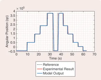
figure 6 A comparison of the experimental and updated model
results of the actuator. First, experimental results are obtained and then numerical simulations are created to obtain a good match by updating the actuator with the time constant xact in (4).
0 10 20 30 40 50 60 70 Time (s) –0.5 0 0.5 1 1.5 2 2.5 3 3.5 4 Angular Position (qc) Reference Experimental Result Model Output × 105
figure 7 moin in the experiments is curve fitted to the data (9). moin
data are calculated via (3) using steady-state pressure values at different operating points and corresponding throat areas, which are dictated manually. A third-order polynomial is fitted to the experimental data. Although mass flow rates are nearly constant at low plant pressures, they decrease at higher pressures because the pressure in the chamber acts like a back pressure for the pres-sure regulator, and high back prespres-sure overcomes the mechanical force in the regulator and reduces the flow rate.
0.2 0.3 0.4 0.5 0.6 0.7 0.8 0.9 1 1.1 Pressure (Normalized) 0.75 0.8 0.85 0.9 0.95 1 1.05 mdo tin (Normalized) Curve Fit Experimental Data
figure 8 A comparison of the open-loop responses of the
experi-mental setup and simulation with the initial (3) and updated plant models (9). the updated model shows a good match with the experimental data. the initial model, based on the constant mass flow rate at the inlet port, fails at high chamber pressures.
25 30 35 40 45 50 Time (s) 0 0.2 0.4 0.6 0.8 1 1.2 1.4 Pressure (Normalized) Initial Model Updated Model Experimental Results
by linearizing the nonlinear plant model and valve equation in (3) and (8), respectively, and ignoring the actuator dynam-ics due to small time constants, compared to that of the pres-sure dynamics. Linearizing (3) around an equilibrium point ( , )P At =( ,P A0 t0) yields
( ) ( ) ,
Po =DPo = -c A2 t0 DP- c P2 0 DAt (10)
where PD =P P- 0 and DAt=At-At0. Defining ap/ -c A2 t0 and bp/ -c P2 0, (10) can be rewritten as
. P a P b Ap p t
Do = D + D (11)
The value of a3 in (8) is much smaller than a1 and a2for meaningful physical parameters, and therefore (8) can be approximated as
( ) .
At. a1+a2i r (12)
It is noted that the valve equation (12) converts the required throat area determined by the pressure controller to the required actuator rotational position, which is provided to the actuator/valve control mechanism as a reference (see Figure 3).
Therefore, together with the actuator time lag ,x the
system model used to develop the controller can be deter-mined as ( ) ( )( ) . W s AP t t s ab e , p t p p s com D D = = -x (13)
ThEORY: COMbINING ADAPTIvE DELAY
COMPENSATION wITh ADAPTIvE TRANSIENT
PERFORMANCE IMPROvEMENT
This section presents the theory behind the controller-termed DR-CRM adaptive controller, which combines delay compensation and adaptive transient performance improve-ment. “Classical Model Reference Adaptive Control” and “Closed-Loop Model Reference Adaptive Control” build on a basic knowledge of control theory to provide the back-ground material necessary to grasp the main ideas of adap-tation and transient performance improvement.
Consider the plant with an input time delay given as
( ) ( )( ) ( ) ( ) ( ), y tp k R spZ s u t W s u t p p p x x = - = - (14)
where yp!0 is the measured output, u!0 is the
con-trol signal, x is the known time delay, and Z sp( ) and
( )
R sp are monic coprime polynomials with orders of m
and ,n respectively. A monic polynomial is one that has the coefficient of one for its highest power term. Coprime polynomials do not share a common root. kp!0 is the
constant gain of the plant. It is noted that the Laplace variable s in (14) is the derivative operator. Similarly, /s1
is the integral operator. The following assumptions are made for the plant:
» System order n is known and the relative degree
. n)=n m- =1
» The sign of kp is known. » Polynomial ( )Z sp is Hurwitz.
The first and the second assumptions are needed in the technical stability proof of the controller and hold true for a large class of systems. The last assumption is required to eliminate any unstable pole-zero cancellation. The ence model dynamics are given with the closed-loop refer-ence model structure as
( ) ( ) ( ) ( ( ) ( )), ( ) ( ), x t A x t b r t L y t y t y t h x t m m m m p m m mT m x = + - + -= o (15) where xm!0n is the state vector, ym!0 is the output, and
r!0 is the reference input for the reference model. Am!0n n# and , ,b L hm m!0n are the state matrix, input
vector, and feedback gain of the reference model and output vector, respectively. Using the Laplace transform, the input–output relationship of the closed-loop reference model can be obtained from (15) as
( ) ( ) ( ) ( ) ( ),
y tm =W s r tm -x +W s e tL 1 (16) where e1=yp-ym is the tracking error and transfer
func-tions are calculated as
( ) ( ) ( )( ), ( ) ( ) ( )( ). W s h sI A b k R sZ s W s h sI A L k R sZ s m mT m m m m m L mT m L m L 1 1 / / - = - = -- (17)
In (17), R sm( ) is a monic polynomial with order ,n while Z sm( )
and Z sL( ) are two monic polynomials with order n-1. km!0 and kL!0 are the gains of the transfer functions.
Note that under model matching conditions [which is the case when a fixed (nonadaptive) controller is design ed to make the closed-loop transfer function equal to the reference model transfer function W sm( ) ,@ the tracking error e1 be -comes zero, which reduces the reference model (16) to
( ) ( ) ( ).
y tm =W s r tm -x (18)
A fixed controller to achieve the model matching condition cannot be designed in the presence of plant uncertainties, since uncertainties are unknown by definition. However, as explained in “Classical Model Reference Adaptive trol” and “Closed-Loop Model Reference Adaptive Con-trol,” in the development of the controllers, the existence of such a controller must be ensured, even though the exact values of the control parameters are unknown.
The state-space description of the plant (14) and the signal generators for the output feedback problem with the controllable ( , )F g pair are given as
Closed-Loop Model Reference Adaptive Control
H
igher adaptation rates in adaptive laws (S9) and (S25) in-crease the speed of adaptation. However, it is observed in simulations and experiments that excessively increasing the adaptation rates causes undesired oscillations. to address this trade-off, the reference model is modified to obtain better transients [40], [S2]–[S9]. closed-loop model reference (crM) adaptive control is one of these methods, proposed in [41]– [43], [S10], [S11], which introduces an error feedback modifi-cation of the reference model to suppress the oscillations for higher adaptation rates (see Figure S4).consider the state-space representation of the reference model dynamics (S14) used in the classical model reference adaptive control (MrAc), given as
( ) ( ) ( ), ( ) ( ). x t A x t b r t y t h x t m m m m m mT m = + = o (S26) As shown in “classical Model reference Adaptive control,”
, ,
Am bm and hm in classical MrAc are chosen such that the
transfer function W sm( )/h sI ATm( - m)-1bm=k Z s R sm( m( )/ m( )) becomes strictly positive real (SPr). in crM adaptive control, the reference model is modified as
( ) ( ) ( ) ( ( ) ( )), ( ) ( ), x t A x t b r t L y t y t y t h x t m m m m p m m mT m = + + -= o (S27) where L!0n is the error feedback gain vector. the
relation-ship between the reference model output ym, the reference ,r and the tracking error e1=yp-ym then becomes
( ) ( ) ( ) ( ) ( ), y tm =W s r tm +W s e tL 1 (S28) where ( ) ( )( ) ( ) , ( ) ( )( ) ( ) . W s k R sZ s h sI A b W s k R sZ s h sI A L m m m m m T m m L L m L m T m 1 1 / / = -= -(S29) Note that in (S28), the Laplace variable s is the derivative operator. Similarly, /s1 is the integral operator. in crM
adap-tive control, there is no modification on the controller structure (S16); therefore, the closed-loop dynamics can again be rep-resented by (S20)–(S22). However, since the crM reference model has an additional error feedback term, the procedure to show stability differs slightly from the MrAc. in this regard, consider the case when the controller parameters become equal to their ideal values, which means that z=0 in (S21). in this case, the ideal closed-loop dynamics become
, , x A x b k r y h x * mn mn mn mn m mnT mn = + = o (S30) w h ere Amn, bmn, a n d hmn are g i ve n i n (S 2 2) a n d xmn= [x* , * , * ]. pT~1T~2T
it was shown for the case of the MrAc that (S30) is a non-minimal representation of the MrAc reference model (S26). therefore, the transfer function obtained from (S30) is
( ) ( )( ) ( ). h sI A b k* k R sZ s W s mn T mn mn m m m m 1 - - = = (S31) recalling that k* k k/ m p
= from the previous section gives
( ) ( )( ) ( ). hmnT sI Amn bmn k R spZ s kk W s m m m p m 1 - - = = (S32)
Using (S21) and (S32), the plant output is ( ) ( )[ ( ) ( ) ( )]. y t kk W s t w t k r t* p m p m zT = + (S33)
Subtracting (S28) from (S33) gives
( ) ( )[ ( ) ( )] ( ). e t kk W s t w t W e t m p m T L 1 = z - 1 (S34)
Solving (S34), the tracking error dynamics are ( ) ( )[ ( ) ( )], e t1 =k W sp e zTt w t (S35) where ( ) ( ) ( ) ( ). W se R sZ sk Z s m L L m = + (S36) Command Tracking Error Reference Model Plant (a) Controller + Command Tracking Error Reference Model Plant (b) Controller + – –
figure s4 (a) classical model reference adaptive control (MrAc), where controller gains are updated by the tracking error
between the plant and reference model outputs. (b) closed-loop MrAc, where tracking error is also fed back to the reference model to improve the transient response.
( ) ( ) ( ), ( ) ( ), ( ) ( ) ( ), ( ) ( ) ( ), x t A x t b u t y t h x t t F t gu t t F t gy t p p p p p pT p 1 1 2 2 x ~ ~ x ~ ~ = + - = = + -= + o o o (19)
where xp!0n is the original plant state vector, ,~ ~1 2!0n are newly created additional state vectors, and yp is the
plant output. Ap!0n n# , ,bp and hp!0n are the plant state
matrix, input vector, and output vector, respectively. F!0n n# is Hurwitz and g!0n.
Defining the future values of the state variables as x trp( )/x tp( +x), y trp( )/y tp( +x), ~r1( )t /~1(t+x) and ( )t (t ), 2 / 2 ~r ~ +x (19) can be rewritten as ( ) ( ) ( ), ( ) ( ), ( ) ( ) ( ), ( ) ( ) ( ), x t A x t b u t y t h x t t F t gu t t F t gy t p p p p p pT p p 1 1 2 2 ~ ~ ~ ~ = + = = + = + ro r r r ro r ro r r (20)
It can be shown that there exist constant controller
param-eters n, n,
1!0 2!0
b) b) and k)!0 such that the controller
( ) ( ) ( ) ( ),
u t T t T t k r t
1 1 2 2
b ~ b ~
= ) r + ) r + ) (21)
satisfies the model matching conditions [39]. Observe that this controller is noncasual because it consists of future va -lues of system states, ( )~r1 t /~1(t+x) and ( )~r2 t /~2(t+x) that are unavailable at the time of control input ( )u t genera-tion. Hence, (21) cannot be realized as is in real applications. However, the unavailable future state values can be predicted using system dynamics, as explained in the following.
It can be shown that the plant output ( )y tp can be ex
-pressed as a linear combination of ~1( ),t ~2( )t as
( ) ( ) ( ),
y tp =cT~1 t +dT~2 t (22)
where ,c d!0n [51]. Substituting (22) into (19) yields
( ) ( ) ( ) ( ) ( ), t t A t t bu t 1 2 1 2 ~ ~ ~ ~ x = + -o o ; E ; E (23) w h e r e A!02n#2n a n d b!02n a r e g i v e n a s A = gcFTF gd+0 T
; E and b=; E Noncasual terms in (21) can g0 .
then be calculated as ( ) ( ) ( ) ( ) ( ) . t t e t t e bu t d A A 1 2 1 2 0 ~ ~ ~ ~ h h = x + h + x -r r ; E ; E
#
(24)When (24) is substituted into (21), the control signal becomes
( )u t T ( )t T ( )t ( ) (u t )d k r t( ), 1 1 2 2 0 a ~ a ~ z h h h = ) + ) + ) + + ) x
-#
(25) where ai)=bi)eAx, ,i=1 2 and ( ) T Te A 1 2 z h) =6b b) ) @ - h are thecorresponding controller parameters. In this form, the con-trol signal is casual and therefore can be implemented.
In the case of unknown plant parameters, the ideal con-trol parameter values , , ( ),a b z hi) i) ) and k) are unknown.
Therefore, the control input ( )u t is rewritten as
( )u t T( )t ( )t T( )t ( )t ( , ) (t u t )d k t r t( ) ( ), 1 1 2 2 0 a ~ a ~ z h h h = + + + + x
-#
(26) where the control parameters ( ), ( ), ( , )a1 t a2 t z ht , and ( )k t are adjusted online based on adaptive laws that are dis-cussed below.Control input (26) can be split into two subsignals as
Polynomials k Z sL L( ) and Z sm( ) are of degree n-1, while R sm( )
is a monic polynomial of degree .n therefore, there is enough
degrees of freedom such that by choosing a proper ,L the
trans-fer function W se( ) can be realized as an SPr transfer function. it can be shown [S10] that after certain transformations, (S35) can be represented in state-space form similar to (S10) in Lemma 1, and therefore the same MrAc adaptive laws given in (S25) can be employed to force the output tracking error e1 to converge to
zero while keeping all system signals bounded. to summarize, crM adaptive laws are identical to MrAc adaptive laws. the er-ror feedback used in the reference model dynamics. the design-er must be careful about selecting the design-error feedback gain L such that the resulting transfer function given in (S36) must be SPr.
REFERENCES
[S2] e. Lavretsky, “reference dynamics modification in adaptive con-trollers for improved transient performance,” in Proc. American Institute
Aeronautics and Astronautics Guidance Navigation and Control Conf.,
2011, p. 6200.
[S3] N. Harl, K. rajagopal, and S. balakrishnan, “Modified state observer for orbit uncertainty estimation,” in Proc. American Institute Aeronautics
and Astronautics Guidance Navigation and Control Conf., 2011, p. 6616.
[S4] e. Lavretsky, “Adaptive output feedback design using asymptotic properties of LQG/Ltr controllers,” IEEE Trans. Autom. Control, vol. 57, no. 6, pp. 1587–1591, 2012.
[S5] V. Stepanyan and K. Krishnakumar, “MrAc revisited: Guaranteed performance with reference model modification,” in Proc. American
Control Conf., pp. 93–98, 2010.
[S6] V. Stepanyan and K. Krishnakumar, “M-MrAc for nonlinear sys-tems with bounded disturbances,” in Proc. Conf. Decision and Control, pp. 5419–5424, 2011.
[S7] t. Yucelen, G. D. L. torre, and e. N. Johnson, “improving transient performance of adaptive control architectures using frequency-limited system error dynamics,” Int. J. Control, vol. 87, no. 11, pp. 2383–2397, 2014. doi: 10.1080/00207179.2014.922702.
[S8] J. Darling, J. Searcy, and S. balakrishnan, “Modified state observer for atmospheric reentry uncertainty estimation,” in Proc. American
In-stitute Aeronautics and Astronautics Guidance Navigation and Control Conf., 2012, p. 4759.
[S9] V. Stepanyan and K. Krishnakumar, “Adaptive control with refer-ence model modification,” J. Guid. Control Dyn., vol. 35, no. 4, pp. 1370–1374, 2012.
[S10] t. Gibson, A. Annaswamy, and e. Lavretsky, “closed-loop ref-erence models for output-feedback adaptive systems,” in Proc. IEEE
European Control Conf., Zurich, 2013, pp. 365–370.
[S11] t. Gibson, A. Annaswamy, and e. Lavretsky, “Adaptive systems with closed-loop reference models, part i: transient performance,” in
Proc. IEEE American Control Conf., Piscataway, NJ, 2013, pp. 3376–
![figure 2 Methods of regulating the fuel flow rate from the gas generator to ram combustor (figures originated from [5] and [6], used with permission): (a) changing the burning area of the propellant, (b) using secondary injection, (c) using a vortex valve](https://thumb-eu.123doks.com/thumbv2/9libnet/5780455.117319/3.850.65.790.700.1029/regulating-generator-combustor-originated-permission-propellant-secondary-injection.webp)
![figure s2 A model reference adaptive control (MrAc) structure, originated from [51]. controller parameters i T 1 ( ), t i T 2 ( ), ( ), t i 0 t and ( )](https://thumb-eu.123doks.com/thumbv2/9libnet/5780455.117319/7.850.79.770.654.1026/figure-reference-adaptive-control-structure-originated-controller-parameters.webp)
![figure s3 Different mechanical elements for throat area change (the figures originated from [5], used with permission)](https://thumb-eu.123doks.com/thumbv2/9libnet/5780455.117319/11.850.63.416.711.999/figure-different-mechanical-elements-throat-figures-originated-permission.webp)