Modularity analysis of a bipartite network for an e-commerce shop

(1)

KADIR HAS UNIVERSITY

GRADUATE SCHOOL OF SCIENCE AND ENGINEERING

MODULARITY ANALYSIS OF A BIPARTITE NETWORK FOR AN

E-COMMERCE SHOP

GRADUATE THESIS

DZORDANA KARINIAUSKAITE

(2)

APPENDIX B D zorda na K ari ni aus ka ite M .S . T he sis 2016 S tude nt ’s F ul l N am e P h.D . (or M .S . or M .A .) T he sis 20 11

(3)

MODULARITY ANALYSIS OF A BIPARTITE NETWORK FOR AN

E-COMMERCE SHOP

DZORDANA KARINIAUSKAITE

Submitted to the Graduate School of Science and Engineering in partial fulfillment of the requirements for the degree of

Master of Science in

MANAGEMENT INFORMATION SYSTEMS

KADIR HAS UNIVERSITY January, 2016

(4)

(5)

ii

“I, Dzordana Kariniauskaite, confirm that the work presented in this thesis is my own. Where information has been derived from other sources, I confirm that this has been indicated in the thesis.”

_______________________

(6)

iii

Abstract

MODULARITY ANALYSIS OF A BIPARTITE NETWORK FOR AN E-COMMERCE SHOP

Dzordana Kariniauskaite

Master of Science in Management Information Systems Advisor: Assoc. Prof. Dr. Mehmet N. Aydın

January,2016

Many real-world systems which are of interest to both researchers and practitioners can be modeled as networks – sets of nodes, representing objects, and links between them, representing the interactions among these objects. One of the most important categories of complex networks in naturally real-world systems is bipartite networks (opposite to general unipartite networks), where nodes can be divided into two disjoint sets such that no two nodes of the same type are connected; there are no links connecting nodes of the same type. The identification of communities in networks is crucial for understanding its underlying structure and behavior. In this study, the bipartite network of Internet shop web platform, where buyers and products represent nodes and purchases made represent links, is analyzed. The analysis is based on the modularity function by means of an open source network analysis and visualization tool Gephi. The twenty biggest modules, including hubs, of the giant component are analyzed in depth. The results of the analysis of category types of product hubs could A PP EN DI X C APPENDIX B

(7)

iv

be used for creating new type of product categories in the e-shop, where the product categories are formed according the most popular product types between communities, leaving behind the traditional marketing methods when the product groups are created considering the characteristics and similarities of the products or the most bought products in the e-shop.

Keywords: Bipartite Network, Modularity, Giant Component, Hubs, Network Analysis

(8)

v

Özet

E-TİCARET MAĞAZASI İÇİN İKİ PARÇALI AĞIN MODÜLER ANALİZİ Dzordana Kariniauskaite

Yönetim Bilişim Sistemleri, Yüksek Lisans Danışman: Doç. Dr. Mehmet N. Aydın

Ocak, 2016

Bilimsel açıdan pek çok gerçek dünya sistemi ağlar – nesneleri temsil eden düğüm kümeleri ve bu nesnelerin birbirleriyle etkileşimlerini simgeleyen bağlantılar- gibi modellenebilir. İnsan sosyal etkinliklerindeki önemli bir karmaşık ağ kategorisi iki tip düğümü olan ve sadece farklı tip düğümlerin bağlanabildiği İkili – Ayrık Düğüm Kümesine Dayalı (Bipartite) Ağlardır. Ağlarda toplulukların tanımlanması onun temel yapısı ve davranışını anlamak için çok önemlidir. Bu çalışmada Internet mağazası web platformunun, müşteriler ile ürünlerin düğümleri ve gerçekleşen satın alımların bağları temsil edildiği, Ayrık Düğüm Kümesine Dayalı ağ analiz edilmiştir. Çözümleme için modülerlik fonksiyonu açık kaynak kodlu bir ağ analiz ve görselleştirme aracı olan Gephi kullanılarak yapılmıştır. Merkez düğüm (hub) ve birlikte dev bileşenin yirmi büyük modülü derinliğine göre çözümlenmiştir.

Anahtar Kelimeler: İkili Ağ, Modülerlik, Dev Bileşen, Merkez Düğüm, Ağ Analizi A PP EN DI X C

(9)

vi

Acknowledgements

I would like to express my appreciation to my advisor Assoc. Prof. Dr. Mehmet N. Aydın for his time and guidance. I also feel very grateful to Asst. Prof. Dr. N. Ziya Perdahçı for his advices and assistance.

I want to express my deepest gratefulness to my family: dad, mum and sister. Thank you for your love, support and faith in me.

Last but not the least, I would like to thank my friends: Meltem Sevim, Seide Ahmadova, Ebru Kayabaşı, Beyza Yiğit, Selcen Arı, Emine Keskin and Enis Kaya individually for their continuous motivation and encouragement. Semiha Nur, thank you for your advices and tips.

A PP EN DI X C

(10)

vii

List of Tables

Table 4.1: Overall list of 20 biggest modules in the giant component ... 21

Table 4.2: Distribution of nodes types in the modules ... 23

Table 4.3: Gender distribution of buyers in modules ... 24

Table 4.4: Distribution of hubs in terms of role attribute (Buyer or Product) of the nodes ... 27

Table 4.5: Gender distribution of buyers’ hubs ... 28

Table 4.6: Distribution of product hubs’ categories in the module ID 74 ... 29

(13)

x

Table 4.25: Distribution of product hubs’ categories in the module ID 82 ... 38 Table 4.26: Product hubs’ categories popularity between modules ... 40

(14)

xi

List of Figures

Figure 2.1: a) undirected network, b) directed network ... 5

Figure 2.2: Bipartite network and its one-mode projections ... 8

Figure 2.4.1: A network with community structure ... 10

Figure 2.4.2: The Zachary karate club network ... 10

Figure 2.5: Modularity formula ... 14

Figure 3.1: The modularity change formula in Louvain algorithm ... 17

Figure 3.2: Modularity change ∆𝑸 for node 0 ... 18

Figure 4.1: The overall view of the giant component network showing products as red nodes, and buyers as turquoise nodes with Force Atlas 2 layout in Gephi ... 22

Figure 4.2: Overall gender distribution of buyers in the giant component ... 23

(15)

1

Chapter 1 Introduction

If someone would ask to characterize the society of 21st century with one adjective, sure enough that connected would be one of the most applicable words for it. We are used to immense interlinked networks that bring electricity, gas, water and television to our homes and that enable us to reach each other almost anywhere in the world by phone, e-mail, and other communication tools. The Internet, especially The World Wide Web takes such important part in our lives that one could barely imagine a day without using it whether it would be for a work or fun.

There are many other systems that are built of components linked together in some way. The Internet, a global computer network, which links billions of devices worldwide by data connections, and human societies, which are groups of people linked by consistent social or acquaintance interactions, are just few examples of such systems.

Many elements of these systems are in the interest area for many scientists. The interest area of the studies can be the nature of individual components of these systems – how human being feels, or how the computer works – as well as the nature of the interactions and connections – the dynamics of human friendships or the communication protocols used on the Internet. There are one more aspect of these systems which in recently years receives more and more attention from academic community. The pattern of connections between components is crucial for behavior of these interacting systems. The pattern of connections can be represented as a network, where the elements of the system are vertices or nodes of the network and the connections the edges.

(16)

2

The network science is a new interdisciplinary science, which has started to emerge just in the end of 20 century. Network science could be defined as the study of the theoretical foundations of network structure and dynamic behavior and the application of networks to many subfields (Lewis, 2011). At the present known subfields include technological networks, social networks, networks of information and biological networks.

To most people a social network means Facebook or other online social networking platform. However, a social network is considered as a network in which nodes represent people, or even group of people, and links represent the interaction or some kind relationship between them (Newman, 2010). Today people are involved in hundreds or even thousands of social networks. We are members of our families, companies we work, organizations we belong, cities we live and this list can be extended endlessly. What is more, we connect to different networks in virtual world everyday by liking new group in Facebook or buying something from a new e-shop. Being able to connect became so important in our lives that we cannot think of a life without social networks anymore.

According to United Nations Department of Economic and Social Affairs in July 2015, world population reached 7.3 billion (The United Nations Department of Economic and Social Affairs, 2015). Despite of it, not once we have heard somebody saying – “It’s a small world”. Newman agrees that in a certain sense it can be true, because “despite the enormous number of people on the planet, the structure of social networks – the map of who knows whom – is such that we are all very closely connected to one another” (2000, p.1).

Stanley Milgram performed one of the first quantitative studies of the structure of social networks in 1967; in 1969 the second study was carried out in collaboration with Jeffrey Travers (Milgram, 1967; Travers & Milgram, 1969). The study was carried out as fallows. The number of letters, addressed to a same person living somewhere in United States, was distributed to a random people. Each of the participants was asked to transfer the message to the addressed person, only by passing the letters to the people, who, in their opinion, could know the targeted person. Messages could be moved only among the people who knew each other on a first-name basis. In the second study the starting person was chosen from Nebraska and the targeted person from Boston in Massachusetts. In the end of the study, Milgram discovered that it had been taken an average of six persons to pass the letter

(17)

3

from Nebraska to Boston. “He concluded, with a somewhat cavalier disregard for experimental niceties, that six was therefore the average number of acquaintances separating the pairs of people involved, and conjectured that a similar separation might characterize the relationship of any two people in the entire world” (Newman, 2000, p.1). This situation is known as six degrees of separation or small world phenomena, which in the language of network science means, “the distance between two randomly chosen nodes in a network is surprisingly short” (Barabasi, 2012, p. 62).

The data used in the study is gathered from one of the e-shop platforms in Turkey. It offers more than million products in ten categories from thousands of different stores to its customers. Everyone who wants to make a purchase in the e-shop firstly has to log in or, if the purchase is made for the first time, open an account providing the basic information such as name, surname, e-mail address and gender. Those who does not want to become a member of e-shop has an option to proceed without opening an account, still they have to provide an e-mail address. Customers who make purchases without signing in to the system cannot track their purchases, learn about special offers and win extra points and coupons. From the network science perspective, the nodes in the network represent buyers and products and the links represent the purchases of products buyers have made. From this data a bipartite network is projected, which means that nodes, buyers and products, can be divided into two disjoint sets where no two nodes of the same type are connected; generally speaking, if buyer has bought a product, there is a link between them, so there is no links connecting only two buyers or two products.

The aim of this paper is to analyze an e-shop network by dividing it into modules, which are more connected to each other in sense of degree.

Is it possible to group goods of different types into categories in terms of its popularity between buyers? If so, what is the best way to do it? Can hub analysis help to identify salient characteristics of these categories?

In this study, I try to answer such questions from a network science perspective. The work consists of five parts. The relevant terminology and previous works are explained in Chapter 2, the method, including tools and the main algorithm used for analysis, is described in Chapter 3, the quantitative results of the analysis are showed in Chapter 4; in Chapter 5 the results, the limitations of the study and the future work is discussed.

(18)

4

Chapter 2 Research Background

2.1. Basic Network Terminology

In its simplest form, a network is a collection of points linked by lines. Newman (2010) describes network as a collection of vertices joined by edges. According to Barabási, “a network is a catalog of a system’s components often called nodes or vertices and directed interactions between them, called links or edges” (2012, p.26). In the scientific literature a network is often referred as a graph. “A graph consists of a set of objects, called nodes, with certain pairs of these objects connected by links called edges” (Easley & Kleinberg, 2010, p.23). However, there is a sly difference between these two terms. The combination of the network, node, and link usually refers to real-world systems, such as, the WWW (the World Wide Web), the metabolic or society networks whereas the terms graph, vertex, and edge are used for mathematical representation of these networks (the web graph, the social graph and etc.) (Barabási, 2012). Because of the distinction between the terms network and graph is rarely made, the terminologies network-graph, node-vertex and link-edge are often used as synonyms of each other. Throughout this paper, the components of the network will be referred as a nodes and connections between the components as a links.

The size of the network (N) is the number of nodes in the network. The number of links (L) in the network represents the total number of interactions between the nodes. Based on the relationship between the two ends of the link (symmetric or

(19)

5

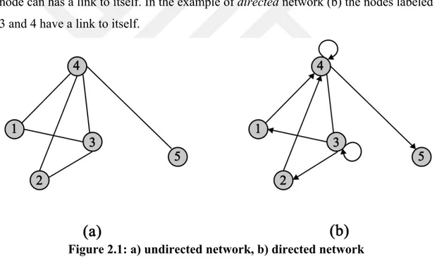
asymmetric), networks can be divided into directed and undirected networks. The network can be described as a directed, if the links between the nodes has a direction; the relationship between the two ends of the link is asymmetric. The links of the directed networks can be defined as a directed links. The examples of such directed networks could be the WWW, citation network, phone calls and etc. The network is being called undirected, when the links simply connects the nodes with direction being unimportant. The Internet, airplane route maps, actor networks, or transmission lines on the power grid are examples of undirected networks. In the Fig. 2.1 below, the example of the directed and undirected networks is given. The nodes of both networks are labeled with integer numbers: 1, 2 and etc. The network (a) is an undirected network, with N=5 and L=6. The network (b) is an example of a directed network. As shown in the example directed network is drawn with links represented by arrows. It is also important to mention that in the directed networks a node can has a link to itself. In the example of directed network (b) the nodes labeled 3 and 4 have a link to itself.

Figure 2.1: a) undirected network, b) directed network

At times, it can be beneficial to depict links of a network as having a strength or value, at most time a real number (Newman, 2010). Hence in the network of the Internet links might have strengths representing the amount of data exchanged between two hosts in the network. In the airport networks, the weighted links show either the number of available seats on direct flight connections between two airports or the number of passengers traveling from one airport to another. For scientific collaboration networks the strength of the link shows the number of coauthored papers between two authors. Contrary to weighted networks unweighted ones have

(20)

6

links where only single link is possible between any two nodes of a network (Barabási, 2012).

The essential property of each node in a network is its degree – the number of links connected to a node (Barabási, 2012; Newman, 2010). It can represent the number of e-mails an individual has sent to its friends, or the number of products a customer bought in electronic shop network. Commonly the degree of node i is denoted as ki (Barabási, 2012; Newman, 2010). For instance, for the undirected network shown in Fig. 2.1 (a) the degrees of nodes are k1=2, k2=2, k3=3, k4=4, k5=1. Logically, the average degree of a network shows the average degree value of the nodes. The degrees of nodes in a network are not the same, to describe the spread in the node degrees a distribution function P(k), which provides the probability that a randomly selected node in the network has degree k, is used (Albert & Barabási, 2002).

Obvious distances characterize the elements of physical systems, for example, the distance between two galaxies in the universe, however, in networks the idea of distance is quite challenging (Barabási, 2012). Indeed, what is the distance between two friends in a social friends network? To answer such a question in networks a path length measure is used (Barabási, 2012). “A path in a network is any sequence of vertices such that every consecutive pair of vertices in the sequence is connected by an edge in the network” (Newman, 2010, p.136). It can intersect itself and pass through the same link many times (Barabási, 2012). So-called shortest path or geodesic path is the path with least number of links between nodes i and j (Barabási, 2012). Differently than in directed networks, the path between i and j in undirected networks is the same as the path between j and i. Network diameter is the distance between the two furthest away nodes. Another important property of paths is average path length – denoted by <d>, is the average number of steps between all possible pairs of nodes in the network (Albert & Barabási, 2002).

The key utility of networks is that they are built to ensure connectedness: they must be capable of establishing a path between any two nodes in a network. A network is said being connected if there is a path between any two pairs of nodes in the network. In disconnected network its parts are called components or clusters. “A component is a subset of nodes in a network, so that there is a path between any two nodes that belong to the component, but one cannot add any more nodes to it that would have the same property” (Barabási, 2012, p.39).

(21)

7 2.2. Adjacency Matrix

In order to fully describe a network, it is important to keep track of its links. For this purpose, the complete list of the network links can be made. “If we denote an edge between vertices i and j by (i, j) then the complete network can be specified by giving the value of n and a list of all the edges” (Newman, 2010, pp.110-11). For instance, the network in the Fig. 2.1 (a) has N=5 nodes and links (1, 3), (1, 4), (2, 3), (2, 4), and (4, 5). However, for mathematical purposes, a better representation of a network is the adjacency matrix. “The adjacency matrix A of a simple graph is the matrix with elements Aij such that

Aij= 1 if there is an edge between vertices 𝑖 and 𝑗,_{0 otherwise" (Newman, 2010, p. 111).}

For example, the adjacency matrix of the network in Fig. 2.1 (a) is

Aij= 0 0 1 1 0 0 0 1 1 0 1 1 0 1 0 1 1 1 0 1 0 0 0 1 0

It is important to notice that for a network with no self-loops the diagonal matrix elements are all zero and that a network is symmetric, if there is a link between i and j then there is a link between j and i (Newman, 2010).

According to Barabási (2012), real networks are sparse. It implies that the adjacency matrices are sparse too. Because of this reason, when a large network is stored in the computer, it is superior to store only the list of links, rather than full adjacency matrix, as a vast part of Aij elements are zero (Barabási, 2012).

(22)

8 2.3. Bipartite Networks

One of the most important categories of complex networks in naturally real- world systems is bipartite networks (opposite to general unipartite networks), where nodes can be divided into two disjoint sets such that no two nodes of the same type are connected; there are no links connecting nodes of the same type. For example, there are two types of node sets, where type a corresponds to movies and type b to actors, two nodes i and j are connected if actor i plays in the movie j; neither two actors nor two movies can be connected. “Bipartite networks appear specialized but are remarkably common” (Larremore et al., 2014, p.1). Examples of bipartite networks could include networks of scientific papers and their authors, social network users and mobile access locations, diseases and genes, plants and pollinators, actors and movies and etc.

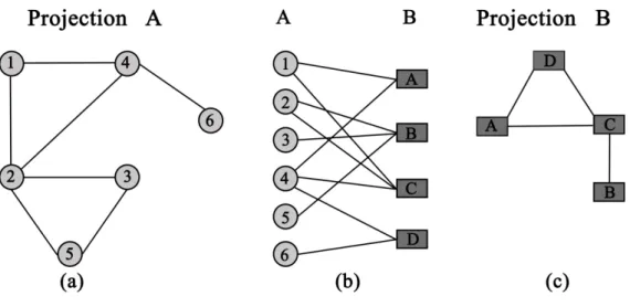
“In many cases, graphs that are fundamentally bipartite are actually studied by projecting them down onto one set of vertices or the other – so called one-mode projections” (Newman, 2003, p.205). These types of projections enable to infer connections between nodes of just one type. For each bipartite network two projections can be generated. Fig. 2.2 shows an example of the two one-mode projections of a small bipartite network.

Figure 2.2: Bipartite network and its one-mode projections (Barabási, 2012) The network (b) is a bipartite network with two sets of nodes; there are 6 nodes of the type A (circles, 1 to 6) and 4 nodes of the type B (rectangular labeled A to D).

(23)

9

The nodes in the A-set connect only the nodes in the B-set. On the left and right sides of the figure two one-mode projections are showed. The projection A, network (a), is obtained by connecting nodes from the A-set to each other if they have direct links with the same node from the B-set in the bipartite network. The projection B, network (c), is obtained by connecting nodes from the B-set to each other if they link to the same A-set node in the bipartite representation.

For mathematical representation of a bipartite network we use so-called incidence matrix, which is an equivalent of an adjacency matrix. “If n is the number of people or other participants in the network and g is the number of groups, then the incidence matrix B is a g x n matrix having elements Bij such that

Bij= 1 if vertex 𝑗 belongs to group 𝑖,

0 otherwise".

For instance, 4×5 incidence matrix of the network shown in Fig. 2.2 (b) is

B=

1 0 0 1 0 0 0 1 1 0 1 0 1 1 0 1 0 0 0 0 0 1 0 1

2.4. Community and Its Detection Algorithms

Community structure is a property, which can be found in most of the real-world networks (Girvan & Newman, 2002). In network science a community is a group of nodes, within which connections are dense, but between which connections are sparser (Newman, 2004). In other words, it means that nodes in the same group have a higher possibility of connecting to each other, than to nodes from other communities (Barabási, 2012). In Fig. 2.4.1 below an example of a network with community structure is shown. There are three communities of densely connected nodes (depicted in circles) in the network and sparse connections between them (light grey lines).

(24)

10

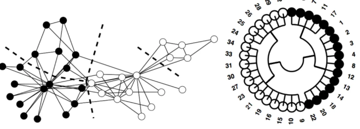
Figure 2.4.1: A network with community structure (Girvan & Newman, 2002) Zachary’s network of karate (Fig. 2.4.2) is a well-known example of a social network and is frequently used as a benchmark for testing community detection algorithms (Zachary, 1977; Porter et al., 2009). The network consists of 34 nodes, members of a karate club. The links of the network shows the interactions between club members outside the club. Because of the conflict between the club president and the instructor, the members of the club have divided into two separate groups. The dashed line in the Fig. 2.4.2 indicates two communities in the network and the black and white circles shows two groups supporting the president and the instructor, respectively.

Figure 2.4.2: The Zachary karate club network (Porter et al., 2009)

“Uncovering the community structure exhibited by real networks is a crucial step towards and understanding of complex systems that goes beyond the local organization of their constituents” (Lancichinetti & Fortunato, 2009, p.1). Because of

(25)

11

this reason, the algorithms for detecting and characterizing community structure have received a great deal of attention in recent years. In this section some community detection techniques will be described.

2.4.1. Traditional Clustering Techniques

The earliest computational efforts to find clusters of similar objects are found in statistics and data mining (Porter et al., 2009). Important methods include partitional clustering techniques such as k-mean clustering, neural network clustering techniques such as self-organizing maps, multidimensional scaling (MDS) techniques such as singular value decomposition (SVD) and principal component analysis (PCA) (Gan et al., 2007). K-means clustering (MacQueen, 1967) is one of the most used clustering algorithms (Gan et al., 2007). It was designed to automatically partition a data set into k groups, where the number of clusters k is fixed (Wagstaff et al., 2001). “It proceeds, for a given initial k clusters, by allocating the remaining data to the nearest clusters and then repeatedly changing the membership of the clusters according to the error function until the error function does not change significantly of the membership of the clusters no longer changes” (Gan et al., 2007, p.161). Multidimensional scaling algorithms are found to be remarkably effective in finding clusters of similar data points in plenty applications, such as voting patterns of legislators and Supreme Court justices (Porter et al., 2009). These kinds of algorithms begin with a matrix that indicates similarities and in return give a coordinate matrix that minimizes a relevant loss function (Porter et al., 2009). Another important example of classical techniques to detect cohesive sets in networks is hierarchical clustering algorithms that are also considered as one of the oldest community detection methods (Newman, 2010; Porter et al., 2009). Hierarchical clustering is an agglomerative technique, which differently from many other community detection algorithms where network is being split apart, begins with the individual vertices of a network and join them to form groups (Newman, 2010).

(26)

12 2.4.2. The Kernighan-Lin Algorithm

This heuristic procedure proposed by Brian Kernighan and Shen Lin deals with the problem of how to partition the nodes of graph G with costs on its edges, into subsets no larger than a given maximum size in order to minimize the total cost of the edges cut (Kernighan & Lin, 1970). In simple words, the algorithm runs as following: at the beginning it randomly divides network into two groups, then tries to find pairs of edges, one from each set, whose interchange would reduce the number of connections (edges) between the groups (Newman, 2010). Despite of the good results in practice and moderately quick running time, the Kernighan-Lin algorithm has one principal disadvantage, which is the specification of the two community sizes before the algorithm starts (Newman, 2004). Newman (2004) found that when algorithm is applied to the Zachary’s karate club in Fig. 2.4.2, it detects the communities perfectly, but in order to get this result, the sizes of the groups should be given as 16 and 18, which are already known sizes of the two groups in which the karate club network have split, in other way, if the sizes of the two groups would be specified differently, the algorithm would produce unlike result. Due to this fact, this algorithm is not suitable to large real-world networks where the sizes of the communities could not be predicted in advance.

2.4.3. Centrality-Based Community Detection

Michelle Girvan and Mark Newman proposed a new approach (Girvan & Newman, 2002) to the detection of communities, based on the sociological notion of betweenness centrality. “First proposed by Freeman, the betweenness centrality of a vertex i is defined as the number of shortest paths between pairs of other vertices which run through i” (Girvan & Newman, 2002, p.3). The Girvan-Newman algorithm is a divisive procedure, which systematically removes the links connecting nodes belonging to different communities, eventually splitting a network into unique groups (Barabási, 2012). The algorithm proceeds as follows: it firstly calculates the betweenness for all links in the network, than removes the link with the largest

(27)

13

betweenness, next it recalculates betweennesses for each link for the altered network and repeats until all links are removed (Girvan & Newman, 2002). When Girvan and Newman applied the algorithm to Zachary’s Karate Club Fig. 2.4.2, they discover that the algorithm divided the club into two groups almost perfectly; only one node was assigned to the wrong group (Barabási, 2012). Nonetheless, as much as centrality-based community detection can look appealing, the running time of the algorithm can be too slow for many large real-world networks (Girvan & Newman, 2002).

2.4.4. k-Clique Percolation

The methods discussed above are used for identifying separated communities, where a node belongs to a single community, however the most actual networks are made of overlapping combined sets of nodes. To give an example, each of us belongs to various different communities, related with our work or personal life (school, family) and so on. Additionally, the members of communities we belong have their own communities, which results in complicated web of nested and overlapping communities themselves. Tamás Vicsek and collaborators proposed an algorithm (Palla et al., 2005) to identify such communities, which brought the attention of the network science community, to the problem of how to interpret the structure of overlapping networks. The method of k-clique percolation (Palla et al., 2005), often called CFinder (Barabási, 2012), is based on the observation that a typical community consists of several fully connected subgraphs that likely share many of their nodes. Vicsek and contributors (2005) define a community as a k-clique-community, which is “a union of all k-cliques (complete subgraphs of size k) that can be reached from each other through a series of adjacent k-cliques (where adjacency means sharing k – 1 nodes)” (p.2).

(28)

14 2.5. Modularity and Resolution Limit

When community structure algorithms are used for the networks where the communities are known ahead of time to measure the quality of used algorithm is easy. However, in practical situations the algorithms are used for the networks where the number of communities cannot be predicted. To solve this problem, Mark Newman and Michelle Girvan introduced a quantity called modularity (Newman & Girvan, 2004) that measures the quality of each division of a network. Modularity is based on the measure of assortative mixing (Newman, 2003), the tendency for nodes with similar characteristics to be connected to other nodes.

“Consider a particular division of a network into k communities. Let us define a 𝑘×𝑘 symmetric matrix e whose element eij is the fraction of all edges in the network that link vertices in community i to vertices in community j” (Newman & Girvan, 2004, p.8). “Then the modularity is defined to be

Figure 2.5: Modularity formula (Newman, 2004)

where 𝐱 indicates the sum of all elements of x” (Newman, 2004, p.6). This quantity measures the fraction of all edges that lie within communities minus the expected value of the same quantity in a network where nodes have the same degrees but connections between nodes are random (Newman, 2010).

The value of modularity shows how good division of network is: the higher Q is, the better is community structure, however, the modularity of a partition cannot be higher than 1 (Barabási, 2012). When the whole network is being considered as a single community Q=0, values other than zero represent partitions from randomness (Newman & Girvan, 2004). “The definition and application of the modularity is independent of the particular community structure algorithm used, and it can therefore also be applied to any other algorithm” (Newman, 2004, p.7).

(29)

15

The anticipation that divisions with the higher modularity corresponds to divisions that more correctly catch the community structure is the starting point of several community detection methods that seek to find partitions with the largest modularity, bypassing the inspection of all possible partitions of a network (Barabási, 2012).

Greedy algorithm, proposed by Mark Newman (2004), is the first community detection method based on modularity maximization (Barabási, 2012). It starts with each node in a separate community on its own and combines communities in pairs, selecting the pairs whose combination will result in the highest increase in Q (Newman, 2004). The principal advantage of the algorithm is its speed, which allows using the algorithm in large networks analysis (Barabási, 2012).

Modularity plays an important role in community detection even though it suffers from resolution limit, as it fails to detect the communities that are smaller than a scale, which depends on the total size of the network and the extent of interconnectedness of its communities (Porter et al., 2009; Fortunato & Barthélemy, 2007). Communities smaller than threshold size are forced into larger communities (Barabási, 2012).

(30)

16

Chapter 3 Method

The data set is received from one of the biggest Turkey’s Internet shops. The nodes in the data are customers and products and the links – the purchases of products customers have made. All records of authorized purchases in May 2015 are analyzed. The bipartite network is projected and the giant connected component of the bipartite network is found using RStudio – the open source software for R. R is a language and environment for statistical computing and graphics. The analysis and visualization of network diagrams and overall views are made with Gephi. It is open source software, which is used for network analysis and visualization (Bastian et al., 2009). In addition, Microsoft Excel is used to sort the data and create tables and diagrams.

The main purpose of the study is to detect community structure of the Internet shop bipartite network. It is achieved using modularity maximization algorithm in Gephi, which is based on Louvain algorithm (Blondel et al., 2008). Etienne Lefebvre was the one who came up with idea for this method. Later, the method was improved and tested together in cooperation with Vincent Blondel, Jean-Loup Guillaume and Renaud Lambiotte and today is known as the “Louvain method” since it was devised when all authors were at the Université catholique de Louvain. The Louvain algorithm is a greedy optimization method that finds high modularity partitions of large networks in a short time and that depicts a community structure for network (Blondel et al., 2008).

The Louvain algorithm is composed of two phases, which are reiterated. Firstly, each node of the network is assigned to a different community, so that in this stage there are as many communities as there are nodes. Next, for each node i, all its

(31)

17

neighbors j are contemplated and the improvement of modularity that would be gained if i would be placed from its own community to the community of j, is evaluated. The node i is placed to the community for which the modularity improvement is biggest, it is also important that this improvement would be positive, contrary, the node i stays in its original community. This process is applied iteratively for all nodes until no further improvement can be accomplished. This concludes the first step of the algorithm. The modularity change ∆𝑄 obtained by moving node i into community 𝐶 is calculated using

Figure 3.1: The modularity change formula in Louvain algorithm (Blondel et al., 2008)

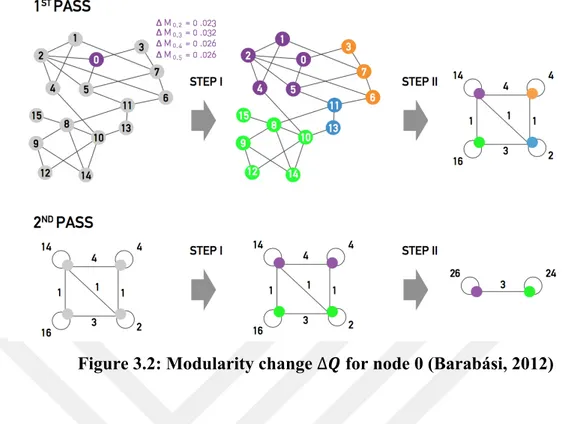
where ∑in is the sum of the weights of the links inside 𝐶 (which Lc for an unweighted network); ∑tot is the sum of the link weights of all nodes in 𝐶 ; ki is the sum of the links incident to node i; ki,in is the sum of the weights of the links from i to nodes in 𝐶 and 𝑚 is the sum of the weights of all links in the network. In the second step of the algorithm a new network whose nodes are the communities identified during the first phase is constructed. The weight of the link between to nodes is the sum of the weight of the links between the nodes in the corresponding communities. Links between nodes of the same community lead to self-loops. After the completion of the second phase, the first phase of the algorithm is reapplied and iterated to the resulting weighted network. The first and second step of the algorithm is called a pass. The number of communities decreases with each pass. The passes are repeated until there are no more changes and the maximum modularity is attained. Fig. 3.2 shows the expected modularity change ∆𝑄 for node 0.

(32)

18

Figure 3.2: Modularity change ∆𝑸 for node 0 (Barabási, 2012)

Fig. 3.2 shows the modularity change for node 0. Firstly, we calculate the change in modularity for node 0 (formula in Fig. 3.1) that would be gained if node 0 would be replaced to its neighbors’ communities. Accordingly, node 0 will join node 3, as the change in modularity is the largest. This process is applied for all nodes. The colors of the nodes correspond to the resulting communities. In the second part of the algorithm the communities obtained in the first phase are aggregated, building a new network of communities. Nodes that belong to the same community are merged into single node, as shown on the top right of Fig. 3.2. This process generates self-loops, which shows the number of links between nodes in the same community. After these two phases, which is called a pass, are completed, the new obtained network is iteratively processed, until there is no improvement in modularity value.

The bipartite network of the data has 441120 nodes and 499436 links. Since the network is quite large and the given representation power of giant component, which includes 318 497 nodes and 411 260 links, we focus on the giant component to conduct network analysis.

After performing the modularity several times, the average number of modules generated changes. The number of modules that have resulted the most is chosen as the number of modules of the network, which in this case are 201. The connection network is represented in general Table 4.1 showing the basic statistics of the 20 biggest modules of the network.

(33)

19

Node degree and path length are two key measures that present effective yet finite insights about the connection network. The node degree in a network is the number of links the node has to other nodes. In such a way, average degree of nodes is the degree, which has the most nodes in the network.

Following tables and diagrams shows the results of analysis of hubs, which is 5% of most connected nodes in modules, as well as the distribution of sex and category of products as product node attributes.

(34)

20

Chapter 4 Results

Gephi does not take the attributes of nodes into consideration while performing modularity analysis. It only contemplates degree of nodes and links. Because of this reason, the attributes of nodes are not being taken into account when calculation is performed. Nonetheless, it is still possible to estimate some basics of the network since the domain is known.

The network examined has 441120 nodes (258429 buyers and 182691 products nodes) and 499436 links. Since in this study the modularity is being examined, only the giant connected component is being analyzed, leaving the sprinkled nodes of the network aside.

4.1 Analysis of Giant Connected Component

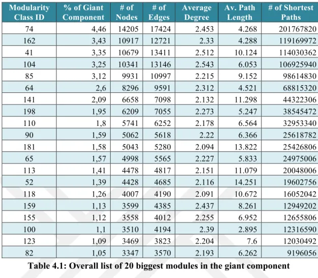
The giant connected component of the network has 318 497 nodes and 411 260 links. It is 72.2 % of the complete network. After performing the modularity in Gephi with resolution 1, which is default value in Gephi, the network was divided into 201 modules. 20 biggest modules were analyzed further. The 20 biggest modules of the giant component correspond to 40.34 % of whole giant connected component. Table 4.1 summarizes the general results of 20 biggest modules.

(35)

21 Modularity Class ID % of Giant Component # of Nodes # of Edges Average Degree Av. Path Length # of Shortest Paths 74 4,46 14205 17424 2.453 4.268 201767820 162 3,43 10917 12721 2.33 4.288 119169972 41 3,35 10679 13411 2.512 10.124 114030362 104 3,25 10341 13146 2.543 6.053 106925940 85 3,12 9931 10997 2.215 9.152 98614830 64 2,6 8296 9591 2.312 4.521 68815320 141 2,09 6658 7098 2.132 11.298 44322306 198 1,95 6209 7055 2.273 5.247 38545472 110 1,8 5741 6252 2.178 6.564 32953340 90 1,59 5062 5618 2.22 6.366 25618782 181 1,58 5043 5280 2.094 13.822 25426806 65 1,57 4998 5565 2.227 5.833 24975006 113 1,41 4478 4817 2.151 11.079 20048006 52 1,39 4428 4685 2.116 14.251 19602756 118 1,26 4007 4190 2.091 10.672 16052042 159 1,13 3599 4385 2.437 8.261 12949202 155 1,12 3558 4012 2.255 6.952 12655806 100 1,1 3510 4194 2.39 2.895 12316590 123 1,09 3469 3823 2.204 7.6 12030492 82 1,05 3347 3570 2.193 6.262 9196056

Table 4.1: Overall list of 20 biggest modules in the giant component As shown in the Table 4.1, the average degree values range from 2.5 until 2.1. The maximum average path length is 14 and the minimum – 4.3. The maximum number of shortest paths is 201767820 the minimum – 9196056.

The average path length displays the average number of steps between all possible pairs of nodes in the network; it measures the efficiency of information transport on the network (Albert & Barabási, 2002). Considering the size of the giant component and its modules, the minimum average path length, which is 4.3, shows quite efficient information transport on the network.

It can be seen in the Table 4.1, that the values of shortest paths are decreasing from the biggest module with the biggest value to the smallest module (20biggest module) with the minimum value.

(36)

22

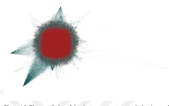
Figure 4.1: The overall view of the giant component network showing products as red nodes, and buyers as turquoise nodes with Force Atlas 2 layout in Gephi

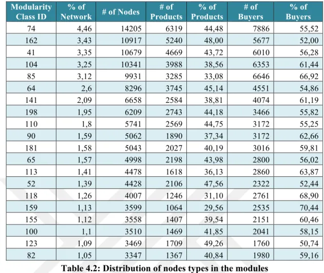
The giant component of the network, shown in Fig. 4.1, is composed of 197020 buyer nodes, which is 62% of the giant connected component, and 121477 product nodes, 38% of the giant connected component. Table 4.2 depicts the number of products and buyers as well as their percentages in the 20 biggest modules of the giant connected component. With no exceptions, buyers form the majority in all modules. However, there are few modules, such as module ID 123, ID 162 and ID 52, where percentage of buyers and products in the modules are very similar. There are no modules composed of one particular type of nodes (Buyers or Products), which makes all modules mixed in terms of type.

(37)

23 Modularity Class ID % of Network # of Nodes # of Products % of Products # of Buyers % of Buyers 74 4,46 14205 6319 44,48 7886 55,52 162 3,43 10917 5240 48,00 5677 52,00 41 3,35 10679 4669 43,72 6010 56,28 104 3,25 10341 3988 38,56 6353 61,44 85 3,12 9931 3285 33,08 6646 66,92 64 2,6 8296 3745 45,14 4551 54,86 141 2,09 6658 2584 38,81 4074 61,19 198 1,95 6209 2743 44,18 3466 55,82 110 1,8 5741 2569 44,75 3172 55,25 90 1,59 5062 1890 37,34 3172 62,66 181 1,58 5043 2027 40,19 3016 59,81 65 1,57 4998 2198 43,98 2800 56,02 113 1,41 4478 1618 36,13 2860 63,87 52 1,39 4428 2106 47,56 2322 52,44 118 1,26 4007 1246 31,10 2761 68,90 159 1,13 3599 1064 29,56 2535 70,44 155 1,12 3558 1407 39,54 2151 60,46 100 1,1 3510 1469 41,85 2041 58,15 123 1,09 3469 1709 49,26 1760 50,74 82 1,05 3347 1367 40,84 1980 59,16

Table 4.2: Distribution of nodes types in the modules

Before purchasing an item in the Internet shop a buyer is being asked to provide his gender. For those who does not want to provide this kind information there is an option “Other”. In the analysis option “Other” is considered as “Unknown” type of gender. In the Fig. 4.2 below, the gender distribution of buyers in the giant connected component is shown.

Figure 4.2: Overall gender distribution of buyers in the giant component 55567, 28% 127387, 65% 14066, 7% Female Male Unknown

(38)

24

As shown in the diagram in the Fig. 4.2 127387 of all buyers are male, which makes 65% of the buyers in the giant connected component, and 55567 of 197020 buyers are female. It is 28% of all buyers. 14066 buyers genders are not known. It forms 7% of all buyers in the giant connected component. Apparently, it can be seen, that male buyers are more active than female buyers in the Internet shop. There are almost 2,3 times more male buyers than female buyers. Even if the 7% of the unknown gender buyers would be considered as female buyers, still male buyers would remain a dominant gender in the network. In this scenario there would be almost 1,9 times more male buyers than female buyers. The following Table 4.3 depicts the gender distribution of buyers in the analyzed modules.

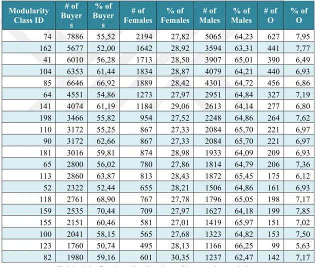
Modularity Class ID # of Buyer s % of Buyer s # of Females % of Females # of Males % of Males # of O % of O 74 7886 55,52 2194 27,82 5065 64,23 627 7,95 162 5677 52,00 1642 28,92 3594 63,31 441 7,77 41 6010 56,28 1713 28,50 3907 65,01 390 6,49 104 6353 61,44 1834 28,87 4079 64,21 440 6,93 85 6646 66,92 1889 28,42 4301 64,72 456 6,86 64 4551 54,86 1273 27,97 2951 64,84 327 7,19 141 4074 61,19 1184 29,06 2613 64,14 277 6,80 198 3466 55,82 954 27,52 2248 64,86 264 7,62 110 3172 55,25 867 27,33 2084 65,70 221 6,97 90 3172 62,66 867 27,33 2084 65,70 221 6,97 181 3016 59,81 874 28,98 1933 64,09 209 6,93 65 2800 56,02 780 27,86 1814 64,79 206 7,36 113 2860 63,87 813 28,43 1872 65,45 175 6,12 52 2322 52,44 655 28,21 1506 64,86 161 6,93 118 2761 68,90 767 27,78 1796 65,05 198 7,17 159 2535 70,44 709 27,97 1627 64,18 199 7,85 155 2151 60,46 581 27,01 1419 65,97 151 7,02 100 2041 58,15 565 27,68 1323 64,82 153 7,50 123 1760 50,74 495 28,13 1166 66,25 99 5,63 82 1980 59,16 601 30,35 1237 62,47 142 7,17

Table 4.3: Gender distribution of buyers in modules

It can be seen from the Table 4.3 once more, that male buyers form the majority of the network. Results show that in all 20 biggest modules of the giant component the male buyers significantly outweigh the female buyers. The percentage of the male buyers in the modules rates from 62 % to 66 %, whereas the female buyers have from 27 % to 30 % of the network. Taking it into account, it

(39)

25

could be said that the number of male buyers is average 2 times bigger than the number of female buyers. Same as the complete giant component, the 20 biggest modules also contain buyers’ nodes of unknown type. All the same, even if unknown buyers would be added to female buyers, again the number of male buyers would be average a bit less than 2 times bigger than the number of female buyers.

In the Fig. 4.3 the types and percentages of product categories in the giant connected component are presented. There are 10 possible categories of products in the Internet shop:

1. NEW_APPAREL_AND_SHOES, 2. NEW_AUTO_AND_MOTO, 3. NEW_BOOK_AND_GAME, 4. NEW_COSMETIC_AND_SELFCARE, 5. NEW_ELECTRONIC, 6. NEW_TRAVEL_AND_ENTERTAINMENT, 7. NEW_JEWELLERY_AND_WATCHES, 8. NEW_HOME_AND_LIFE, 9. NEW_MOTHER_AND_BABY, 10. NEW_SPORT_AND_OUTDOOR.

The most popular product category in the giant connected component is NEW_ELECTRONIC. 30297 products, which are 25% of all products, were bought from NEW_ELECTRONIC category. Second favored category between buyers is NEW_HOME_AND_LIFE category. In this category 23126 products were bought, it is 19% of all products. The third most selected category is NEW_APPAREL_AND_SHOES. From this category 18852 products were bought which is 16% of all products. The following categories according the number of bought items from it: NEW_COSMETIC_AND_SELFCARE with 18852 products

(16%), NEW_SPORT_AND_OUTDOOR – 13303, 11%,

NEW_BOOK_AND_GAME – 9845, 8%, NEW_AUTO_AND_MOTO – 7195, 6%,

NEW_MOTHER_AND_BABY – 6416, 5%,

NEW_JEWELLERY_AND_WATCHES – 6029, 5% and

NEW_TRAVEL_AND_ENTERTAINMENT with 33 products (0%). The difference of number of items bought in 9th_{and 10}th_{most popular categories is very big: 6029} products bought from the 9th category and only 33 products from 10th one. It could be stated that the NEW_TRAVEL_AND_ENTERTAINMENT category is really

(40)

26

unpopular between buyers in the Internet shop and that the Internet shop should to consider taking additional means for increasing sales in this category or completely stop selling these products.

Figure 4.3: Distribution of product types categories in the giant component

4.2 Analysis of The Hubs

In the second part of the analysis, the hubs of 20 biggest modules of the giant connected component were analyzed. In the study the 5 % of the nodes with the highest degrees were chosen as hubs. Table 4.4 displays the products and buyers distribution in the hubs as well as the number of hubs in the 20 biggest giant connected component’s modules.

30297, 25% 23126, 19% 18852, 16% 13303, 11% 9845, 8% 7195, 6% 6416, 5% 6381, 5% 6029, 5% 33, 0% NEW_ELECTRONIC NEW_HOME_AND_LIFE NEW_APPAREL_AND_SHOES NEW_COSMETIC_AND_SELFCAR E NEW_SPORT_AND_OUTDOOR NEW_BOOK_AND_GAME NEW_AUTO_AND_MOTO NEW_MOTHER_AND_BABY NEW_JEWELLERY_AND_WATCHE S NEW_TRAVEL_AND_ENTERTAIN MENT

(41)

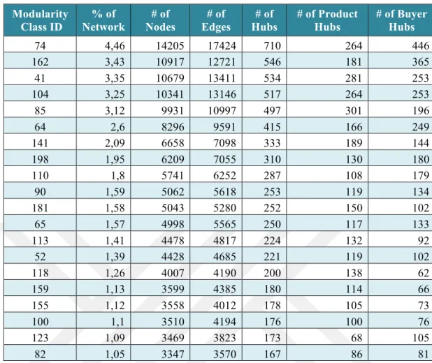
27 Modularity

Class ID Network % of Nodes # of Edges # of Hubs # of # of Product Hubs # of Buyer Hubs

74 4,46 14205 17424 710 264 446 162 3,43 10917 12721 546 181 365 41 3,35 10679 13411 534 281 253 104 3,25 10341 13146 517 264 253 85 3,12 9931 10997 497 301 196 64 2,6 8296 9591 415 166 249 141 2,09 6658 7098 333 189 144 198 1,95 6209 7055 310 130 180 110 1,8 5741 6252 287 108 179 90 1,59 5062 5618 253 119 134 181 1,58 5043 5280 252 150 102 65 1,57 4998 5565 250 117 133 113 1,41 4478 4817 224 132 92 52 1,39 4428 4685 221 119 102 118 1,26 4007 4190 200 138 62 159 1,13 3599 4385 180 114 66 155 1,12 3558 4012 178 105 73 100 1,1 3510 4194 176 100 76 123 1,09 3469 3823 173 68 105 82 1,05 3347 3570 167 86 81

Table 4.4: Distribution of hubsin terms of role attribute (Buyer or Product) of the nodes

The distribution of products and buyers in the hubs of modules differs from the overall giant connected component distribution of the same subject. Contrary to the distribution of products and buyers in the giant connected component where the buyers formed the majority of modules, in the modules in terms of type of hubs any kind of significantly dominant pattern can not be seen since there are 11 hubs with the products as a majority and 9 hubs where the buyers takes the top. There is one module ID 118, which has more than 2 times bigger number of product hubs than the number of buyer hubs (138 product hubs and 62 buyer hubs).

(42)

28 Modularity Class ID # of Hubs # of Buyers # of Males % of Males # of Females % of Femal es # of O % of O 74 710 446 282 63,23 131 29,37 33 7,4 162 546 365 231 63,29 110 30,14 24 6,58 41 534 253 170 67,19 67 26,48 16 6,32 104 517 253 162 64,03 76 30,04 15 5,93 85 497 196 109 55,61 72 36,73 15 7,65 64 415 249 167 67,07 73 29,32 9 3,61 141 333 144 93 64,58 38 26,39 13 9,03 198 310 180 117 65 45 25 18 10 110 287 179 121 67,60 43 24,02 15 8,38 90 253 134 84 62,69 42 31,34 8 5,97 181 252 102 67 65,69 27 26,47 8 7,84 65 250 133 83 62,41 42 31,58 8 6,02 113 224 92 55 59,78 32 34,78 5 5,43 52 221 102 67 65,69 30 29,41 5 4,90 118 200 62 41 66,13 17 27,42 4 6,45 159 180 66 45 68,18 19 28,79 2 3,03 155 178 73 50 68,49 19 26,03 4 5,48 100 176 76 49 64,47 23 30,26 4 5,26 123 173 105 68 64,76 33 31,43 4 3,81 82 167 81 58 71,60 18 22,22 5 6,17

Table 4.5: Gender distribution of buyers’ hubs

Table 4.5 shows the overall gender distribution of buyers’ hubs in the 20 biggest modules. The results do not differ much from the overall gender distribution of buyers showed in Table 4.3. Again male buyers’ hubs form the majority. In the module ID 82 male buyers contain more than 71 % of all buyer hubs; this kind of result was not observed in the overall gender distribution of buyers in all 20 modules. In the following 20 tables the distribution of bought products in every category of hubs is shown. The tables displayed from the biggest module product hub to the smallest one.

Table 4.6 shows the distribution of product hubs’ categories in the biggest module ID 74. It can be seen that the most popular products are from the NEW_HOME_AND_LIFE category, from which more than a quarter of all products were sold. Second the most popular group is NEW_ELECTRONIC, which contains almost 18 % of a network. The least popular category in this module is NEW_TRAVEL_AND_ENTERTAINMENT, which no products sold at all.

(43)

29

Modularity

Class ID Product Category # of Nodes %

74 NEW_HOME_AND_LIFE 71 26,89 NEW_ELECTRONIC 47 17,80 NEW_APPAREL_AND_SHOES 33 12,50 NEW_SPORT_AND_OUTDOOR 29 10,98 NEW_MOTHER_AND_BABY 26 9,85 NEW_COSMETIC_AND_SELFCARE 22 8,33 NEW_JEWELLERY_AND_WATCHES 15 5,68 NEW_AUTO_AND_MOTO 11 4,17 NEW_BOOK_AND_GAME 10 3,79 NEW_TRAVEL_AND_ENTERTAINMENT 0

Table 4.6: Distribution of product hubs’ categories in the module ID 74 Table 4.7 shows the distribution of product hubs’ categories in the module ID 162. The biggest category is NEW_HOME_AND_LIFE; it contains more than a quarter of all sold products in this module. The second one is NEW_APPAREL_AND_SHOES with 19% and the third NEW_ELECTRONIC and forth NEW_COSMETIC_AND_SELFCARE categories are similar size. The sizes of the rest categories are almost the same, from 12 to 10 nodes. Again as in the previous module ID 74 no products were chosen from the NEW_TRAVEL_AND_ENTERTAINMENT category.

Modularity

Class ID Product Category # of Nodes %

162 NEW_HOME_AND_LIFE 46 25,41 NEW_APPAREL_AND_SHOES 34 18,78 NEW_ELECTRONIC 23 12,71 NEW_COSMETIC_AND_SELFCARE 22 12,15 NEW_BOOK_AND_GAME 12 6,63 NEW_MOTHER_AND_BABY 12 6,63 NEW_AUTO_AND_MOTO 11 6,08 NEW_JEWELLERY_AND_WATCHES 11 6,08 NEW_SPORT_AND_OUTDOOR 10 5,52 NEW_TRAVEL_AND_ENTERTAINMENT 0

Table 4.7: Distribution of product hubs’ categories in the module ID 164 Table 4.8 shows the distribution of product hubs’ categories in the module ID 41. The first most popular category is NEW_ELECTRONIC with 22 % of product nodes. The second and third categories (NEW_ELECTRONIC and

(44)

30

NEW_APPAREL_AND_SHOES) have the same number of nodes, which is 45; it makes 16 % of the network.

Modularity

Product Category # of Nodes %

Class ID 41 NEW_ELECTRONIC 63 22,42 NEW_APPAREL_AND_SHOES 45 16,01 NEW_HOME_AND_LIFE 45 16,01 NEW_COSMETIC_AND_SELFCARE 28 9,96 NEW_BOOK_AND_GAME 26 9,25 NEW_JEWELLERY_AND_WATCHES 21 7,47 NEW_MOTHER_AND_BABY 20 7,12 NEW_SPORT_AND_OUTDOOR 19 6,76 NEW_AUTO_AND_MOTO 14 4,98 NEW_TRAVEL_AND_ENTERTAINMENT 0

Table 4.8: Distribution of product hubs’ categories in the module ID 41 Table 4.9 shows the distribution of product hubs’ categories in the module ID 104. NEW_HOME_AND_LIFE category is the most popular in this module. It contains 23% of all products. The second NEW_ELECTRONIC and third NEW_APPAREL_AND_SHOES categories contain almost similar percentage of products. It differs by 1.5 %. NEW_TRAVEL_AND_ENTERTAINMENT category again is most unpopular, however in this hub 1 product from this category was sold, which makes 0.38% of network.

Modularity

Class ID 104 NEW_HOME_AND_LIFE 61 23,11 NEW_ELECTRONIC 44 16,67 NEW_APPAREL_AND_SHOES 40 15,15 NEW_COSMETIC_AND_SELFCARE 30 11,36 NEW_AUTO_AND_MOTO 22 8,33 NEW_SPORT_AND_OUTDOOR 18 6,82 NEW_BOOK_AND_GAME 17 6,44 NEW_JEWELLERY_AND_WATCHES 16 6,06 NEW_MOTHER_AND_BABY 15 5,68 NEW_TRAVEL_AND_ENTERTAINMENT 1 0,38

Table 4.9: Distribution of product hubs’ categories in the module ID 104 Table 4.10 shows the distribution of product hubs’ categories in the module ID 85. The most popular category in this module is NEW_ELECTRONIC. It contains 19 % of the network. The second (NEW_COSMETIC_AND_SELFCARE) and third

(45)

31

(NEW_HOME_AND_LIFE) categories differ just by 1 node. Second category has 52 nodes, which makes more than 17 % of the network and third one has 51 nodes, which forms almost 17 % of the network. The least chosen category again is NEW_TRAVEL_AND_ENTERTAINMENT; no products were bought from this group.

Modularity

Class ID 85 NEW_ELECTRONIC 58 19,27 NEW_COSMETIC_AND_SELFCARE 52 17,28 NEW_HOME_AND_LIFE 51 16,94 NEW_APPAREL_AND_SHOES 45 14,95 NEW_SPORT_AND_OUTDOOR 27 8,97 NEW_AUTO_AND_MOTO 21 6,98 NEW_BOOK_AND_GAME 21 6,98 NEW_MOTHER_AND_BABY 16 5,32 NEW_JEWELLERY_AND_WATCHES 10 3,32 NEW_TRAVEL_AND_ENTERTAINMENT 0

Table 4.10: Distribution of product hubs’ categories in the module ID 85 Table 4.11 shows the distribution of product hubs’ categories in the module ID 64. NEW_HOME_AND_LIFE category contains almost 28 % of products and is the most chosen between buyers. The second one is NEW_ELECTRONIC category, which is 9 % smaller than first category. It has 19 % of products. There are no products sold from NEW_TRAVEL_AND_ENTERTAINMENT category.

Modularity

Class ID 64 NEW_HOME_AND_LIFE 46 27,71 NEW_ELECTRONIC 31 18,67 NEW_APPAREL_AND_SHOES 23 13,86 NEW_COSMETIC_AND_SELFCARE 17 10,24 NEW_BOOK_AND_GAME 13 7,83 NEW_SPORT_AND_OUTDOOR 13 7,83 NEW_MOTHER_AND_BABY 9 5,42 NEW_AUTO_AND_MOTO 8 4,82 NEW_JEWELLERY_AND_WATCHES 6 3,61 NEW_TRAVEL_AND_ENTERTAINMENT 0

Table 4.11: Distribution of product hubs’ categories in the module ID 64 Table 4.12 shows the distribution of product hubs’ categories in the module ID 141. The most popular category in this hub is NEW_HOME_AND_LIFE. It contains

(46)

32

22 % of all products. The second most popular category (NEW_APPAREL_AND_SHOES) has 19 % of all products. Again, there are no products sold from NEW_TRAVEL_AND_ENTERTAINMENT category.

Modularity

Class ID 141 NEW_HOME_AND_LIFE 42 22,22 NEW_APPAREL_AND_SHOES 36 19,05 NEW_ELECTRONIC 31 16,40 NEW_COSMETIC_AND_SELFCARE 23 12,17 NEW_BOOK_AND_GAME 15 7,94 NEW_SPORT_AND_OUTDOOR 15 7,94 NEW_AUTO_AND_MOTO 14 7,41 NEW_JEWELLERY_AND_WATCHES 8 4,23 NEW_MOTHER_AND_BABY 5 2,65 NEW_TRAVEL_AND_ENTERTAINMENT 0

Table 4.12: Distribution of product hubs’ categories in the module ID 141 Table 4.13 shows the distribution of product hubs’ categories in the module ID 198. The first three most popular categories are as fallows: NEW_HOME_AND_LIFE (30 %), NEW_APPAREL_AND_SHOES (21 %) and NEW_ELECTRONIC (19 %). NEW_TRAVEL_AND_ENTERTAINMENT category has no products sold.

Modularity

Class ID 198 NEW_HOME_AND_LIFE 30 23,08 NEW_APPAREL_AND_SHOES 21 16,15 NEW_ELECTRONIC 19 14,62 NEW_COSMETIC_AND_SELFCARE 18 13,85 NEW_MOTHER_AND_BABY 11 8,46 NEW_AUTO_AND_MOTO 10 7,69 NEW_BOOK_AND_GAME 9 6,92 NEW_JEWELLERY_AND_WATCHES 8 6,15 NEW_SPORT_AND_OUTDOOR 4 3,08 NEW_TRAVEL_AND_ENTERTAINMENT 0

Table 4.13: Distribution of product hubs’ categories in the module ID 198 Table 4.14 shows the distribution of product hubs’ categories in the module ID 110. The first three most popular categories are the same as in the previous module (ID 198), only their sizes differ the NEW_HOME_AND_LIFE category is first (22 %), the NEW_ELECTRONIC is second (21 %) and the

(47)

33

NEW_APPAREL_AND_SHOES category (15 %) is third. The other categories in the comparison with the first three biggest categories are quite small. It ranges from 9 % to 0 %.

Modularity

Class ID 110 NEW_HOME_AND_LIFE 24 22,22 NEW_ELECTRONIC 23 21,30 NEW_APPAREL_AND_SHOES 17 15,74 NEW_COSMETIC_AND_SELFCARE 9 8,33 NEW_SPORT_AND_OUTDOOR 9 8,33 NEW_JEWELLERY_AND_WATCHES 8 7,41 NEW_BOOK_AND_GAME 7 6,48 NEW_MOTHER_AND_BABY 6 5,56 NEW_AUTO_AND_MOTO 5 4,63 NEW_TRAVEL_AND_ENTERTAINMENT 0

Table 4.14: Distribution of product hubs’ categories in the module ID 110 Table 4.15 shows the distribution of product hubs’ categories in the module ID 90. In this module the first category NEW_ELECTRONIC and the second category NEW_HOME_AND_LIFE is of very similar size (26 nodes and 24 nodes). The third biggest category NEW_APPAREL_AND_SHOES and the forth NEW_COSMETIC_AND_SELFCARE category also contains a similar number of nodes (20 and 18). The rest categories’ sizes range from 9 % to 0 %.

Modularity

Class ID 90 NEW_ELECTRONIC 26 21,85 NEW_HOME_AND_LIFE 24 20,17 NEW_APPAREL_AND_SHOES 20 16,81 NEW_COSMETIC_AND_SELFCARE 18 15,13 NEW_SPORT_AND_OUTDOOR 11 9,24 NEW_AUTO_AND_MOTO 6 5,04 NEW_BOOK_AND_GAME 5 4,20 NEW_JEWELLERY_AND_WATCHES 5 4,20 NEW_MOTHER_AND_BABY 4 3,36 NEW_TRAVEL_AND_ENTERTAINMENT 0

Table 4.15: Distribution of product hubs’ categories in the module ID 90 Table 4.16 shows the distribution of product hubs’ categories in the module ID 181. The biggest NEW_HOME_AND_LIFE category has 24 % of all products and the second NEW_ELECTRONIC category is 6% smaller than the first one. The third