Coordination of pricing and production-scheduling decisions in supply chains

(1)

COORDINATION OF PRICING AND

PRODUCTION-SCHEDULING DECISIONS IN

SUPPLY CHAINS

A THESIS

SUBMITTED TO THE DEPARTMENT OF INDUSTRIAL ENGINEERING AND THE INSTITUTE OF ENGINEERING AND SCIENCE

OF BILKENT UNIVERSITY

IN PARTIAL FULFILLMENT OF THE REQUIREMENTS FOR THE DEGREE OF

MASTER OF SCIENCE

By

Muzaffer Mısırcı September, 2008

(2)

I certify that I have read this thesis and that in my opinion it is fully adequate, in scope and in quality, as a thesis for the degree of Master of Science.

Prof. Dr. İhsan Sabuncuoğlu (Advisor)

Assist. Prof. Dr. Ayşegül Toptal (Co-Advisor)

Assist. Prof. Dr. Mehmet Rüştü Taner

Assist. Prof. Dr. Nagihan Çömez

Approved for the Institute of Engineering and Science:

Prof. Mehmet Baray

(3)

Abstract

COORDINATION OF PRICING AND

PRODUCTION-SCHEDULING DECISIONS IN

SUPPLY CHAINS

Muzaffer Mısırcı M.S. in Industrial Engineering

Supervisor: Prof. İhsan Sabuncuoğlu, Assist. Prof. Ayşegül Toptal September 2008

Integration of various business functions ranging from procurement and distribution activities to customer relations has gained importance due to the progressively increasing global and domestic competitive pressures. As a consequence, many firms have set out to design, develop, and install their supply chain solutions.

The existing literature on wholesale price contracts takes into account the ordering and inventory holding component of the total. However, the impact of capacity considerations is overlooked in the coordination of replenishment decisions.

In this thesis, our objective is to synchronize the production planning and pricing decisions in buyer-vendor systems. In order to achieve this objective, the vendor quotes a price schedule that is a function of delivery time and order quantity. This price schedule stimulates the manipulation of buyer’s order time and quantities so as to minimize vendor’s total costs without changing the buyers’ profit position.

(4)

Özet

TEDARİK ZİNCİRLERİNDE

FİYATLANDIRMA VE ÜRETİM-PLANLAMA

KARARLARININ KOORDİNASYONU

Muzaffer Mısırcı

Endüstri Mühendisliği Yüksek Lisans

Tez Yöneticisi: Prof. İhsan Sabuncuoğlu, Yrd. Doç. Dr. Ayşegül Toptal Eylül 2008

Giderek ağırlaşan iç ve dış rekabet koşulları firmaların satın alma faliyetlerinden, ürünlerinin dağıtımına ve müşteri ilişkilerine kadar olan iş süreçlerinin entegrasyonunu zorunlu hale getirmiştir. Bu yüzden günümüzde çok sayıda firma tedarik zinciri yönetimi sistemlerini kurmaya başlamışlardır. Ancak bu konuda çok gelişmiş ve her sektörün ihtiyacını karşılayan maliyet etkin çözümlerin olmayışı önemli bir eksiklik olarak ortaya çıkmaktadır.

Bu konu ile ilgili geçmişte yapılan bilimsel çalışmalar, alıcı ve satıcı arasındaki ticari ilişkinin koordinasyonunu sipariş verme ve envanter tutma maliyetleri çerçevesinde ele almakla beraber, satıcı firmanın olası kapasite kısıtlarını göz ardı etmektedir.

Biz bu tezde tedarikçi ve müşteri arasındaki koordinasyonun sağlanmasında önemli bir etken olan üretim planlama ve fiyatlandırma kararlarını sistematik bir yaklaşımla karar sürecıne dahil etmeyi amaçlıyoruz. Bu sistematik yaklaşımın temelinde yatan düşünce, tedarikçi firmanın miktara dayalı fiyat politikasını belirlerken, müşterilerden gelecek sipariş profilini kendi üretim maliyetlerini azaltacak yönde etkilemesidir. İstenen etkinin gerçekleşmesi için belirlenen fiyat politikası, müşterilerin yeni talep profilleri sonunda oluşacak kar durumlarını azaltmamalıdır.

Anahtar Kelimeler: tedarik zinciri, üretim planlama, fiyatlandırma, fiyat menüsü, koordinasyon

(5)

(6)

Acknowledgement

I would like to express my sincere gratitude to Prof. İhsan Sabuncuoğlu, Asst. Prof. Ayşegül Toptal and Asst. Prof. Mehmet Rüştü Taner for their instructive comments and encouragements in this thesis work. Their valuable suggestions in the supervision of the thesis will guide me throughout all my academic life.

I am indebted to Asst. Prof. Nagihan Çömez for accepting to review this thesis.

I would like to thank to Mehmet Mustafa Tanrıkulu, Fatih Safa Ereneay, Hakan Gültekin, Fazıl Paç, Gülay Samatlı, Ahmet Camcı, Çağdaş Büyükkaramıklı, Çağrı Latifoğlu, Sinan Gürel, Ayşegül Altın and my other friends for their helps and morale support during my graduate study.

Finally, I would like to express my deepest gratitude to my family for their understanding and patience during my graduate life.

(7)

LIST OF FIGURES

FIGURE 1: PRODUCTION AND DEMAND PERIODS... 10 FIGURE 2: PROFITABILITY OF CONTRACT DTDP AS FUNCTION OF NUMBER OF DUE-DATES.………... 29 FIGURE 3: THE EFFECT OF PRODUCTION COST ON THE PERFORMANCE OF CONTRACT DTDP RELATIVE TO THAT OF FWTP... 32 FIGURE 4: THE EFFECT OF INVENTORY COST ON THE PERFORMANCE OF CONTRACT DTDP RELATIVE TO THAT OF FWTP... 33 FIGURE 5: THE EFFECT OF TARDINESS COST ON THE PERFORMANCE OF CONTRACT DTDP RELATIVE TO THAT OF FWTP... 34 FIGURE 6: THE EFFECT OF PRODUCTION CAPACITY WITHIN THE DEMAND PERIOD... 35 FIGURE 7: THE EFFECT OF STOCHASTICITY ON THE PERFORMANCE OF CONTRACT DTDP RELATIVE TO THAT OF FWTP... 36

(9)

LIST OF TABLES

Table 1: The raw data containing all instances in experimental design ... 41

Table 2: Summary of the data used for bar charts in the numerical results ... 68

Table 3: The data for endogenous variable number of due-dates………... 69

(10)

C h a p t e r 1

INTRODUCTION

Supply chain management is a relatively new area in manufacturing and service operations management. The need for managing the materials and information across the supply chain originates from the fact that the actions taken by one member of the chain can influence the profitability of the others. It has been shown in various studies that significant savings can be achieved due to coordinating the independently made decisions of the parties in supply chain systems. Therefore, many firms have set out to design, develop, and install their supply chain solutions to cope with the increasing global and domestic competitive pressures. The investment on supply chain optimization amounts to a scale of three million dollars in Turkey and to one billion dollar around the world. This indicates a need and an opportunity for the development of effective decision-support tools for supply chain management.

The evolution of supply chain management initiates from the classical multi-echelon inventory theory. The studies on multi-multi-echelon inventory systems (e.g., Clark and Scarf (1960), Federgruen and Zipkin (1984),) suggest that the companies make their inventory replenishment decisions jointly. The major pursuit of the more recent studies is to introduce certain mechanisms into supply chain systems for alligning the individual incentives of the companies with the system performance, while still allowing independent decision making. In view of this trend, much of the recent research effort on supply chain management has

(11)

been spent to develop mechanisms for coordinating the system and to evaluate their effectiveness in different settings.

As it will be discussed in detail in the following section, a majority of the studies that could fall into this second body of research, takes minimization of inventory related costs as a performance measure. Few studies appeared in the more recent literature on supply chain management which consider other supply chain functionalities in addition to inventory management . For example, Toptal and Çetinkaya (2006) investigate the contractual agreements for supply chain coordination under the consideration of the vendor’s inbound and outbound transportation costs.

In addition to inventory holding and transportation, another important function that affects supply chain costs significantly, is production scheduling. It is important to note that, the above mentioned literature overlooks production capacity and scheduling considerations at the vendor/manufacturer. However, in real life, a manufacturer may accept/reject orders on the basis of capacity constraints and he/she may quote varying wholesale prices for orders with different due-dates depending on resource availability. Better yet, he/she may adjust the wholesale prices to change the ordering behaviors of the buyers/retailers for increasing supply chain efficacy through better utilization of the capacity. This, in fact, is the opportunity at stake, which also, is the motivation to our study.

In this thesis, a single period, stochastic demand environment with one vendor/manufacturer and multiple buyers/retailers is considered, and the production capacity at the vendor1 is modeled explicitly. The vendor’s manufacturing plant is regarded as a single machine, and his/her earliness and tardiness costs resulting from the aggregate scheduling decisions are taken into account in computing his/her expected profits. The main objective of the thesis is

1_{In the remaining parts of the thesis, “vendor” and “manufacturer”, and “buyer” and “retailer” will}

(12)

the design of contracts between the vendor and the buyers under careful consideration of the vendor’s production capacity. To achive this objective, a novel contract type is proposed and is compared to a more traditional one. The proposed contract allows the vendor to offer delivery time dependent wholesale prices to the retailers. The vendor considers the production capacity and scheduling decisions explicitly in determining the wholesale prices, and plans to deliver all accepted orders on time. Furthermore, the models constructed for this contract, enable the computation of wholesale prices which maximize the vendor’s net profits while maintaining the buyers’ potential profits that would result from their independent decisions. Then, the proposed contract type is compared to a more traditional one which allows the vendor to complete and deliver the accepted orders later than their promised duedates, while making a fixed payment (i.e., penalty cost) to the related retailer(s) in compensation. In this contractual agreement, wholesale prices do not depend on delivery times. Through an extensive numerical analysis, it is shown that considerable savings can be achieved by the proposed contractual agreement.

The organization of the thesis will be as follows. In the next chapter, a review of the literature is provided. In Chapter 3, the two contractual agreements are formulated, and the manufacturer’s and the retailers’ profit functions in each contract are derived. The following chapter analyzes the manufacturer’s profit maximization problem in the proposed contract. Chapter 5 presents the experimental design and discusses the numerical results. Finally, in Chapter 6, general conclusions of this study are summarized.

(13)

C h a p t e r 2

LITERATURE REVIEW

This study is closely related to the body of work on multi-echelon inventories, supply chain management and contracting theory. Optimization of serial inventory systems, i.e., multi-echelon inventories, dates back to 1960s with the pioneering work of Clark and Scarf (1960) for a stochastic demand environment. Following this study, numerous other researchers investigated the problem under different assumptions (e.g., Federgruen and Zipkin (1984), Debodt and Graves (1985), Rosling (1985)). Federgruen (1993) provides an excellent review of the literature on multi-echelon inventories. A common property of all the studies in this review paper is that, they model a decision-making system in which the suppliers and the retailers make their inventory and production decisions jointly, in a centralized manner. However, in real life, the implementation of a centralized model is very difficult unless the companies belong to the same corporation, or the vendor manages and owns the inventory at the buyer(s) as in a VMI (Vendor Managed Inventory) system. Çetinkaya and Lee (2000), Toptal et al. (2003) are some examples of recent papers that study the coordination problem in VMIs.

An alternative approach to the centralized modeling is the decentralized modeling, in which the supply chain players make their decisions on their own, with limited information sharing. However, it is known that the decentralized modeling approach results in a reduction of total system profits relative to the centralized modeling approach. In other words, the independent action of one

(14)

member of the supply chain may make others worse. This concept is referred to as “Double Marginalization” (Spengler, 1950) in the literature. One of the earlier studies in operations management which illustrate the gap between the two modeling approaches, is by Goyal (1976). Starting from this work, there has been an increasing trend in supply chain studies to investigate ways for improving the outcome of the decentralized model for a system, by using the corresponding centralized model as a benchmark. The idea of aligning the individual incentives for all parties in a decentralized model with those of the centralized solution is known as channel coordination in the literature. This is done by manipulating the system parameters such as wholesale price, salvage value etc., a.k.a., coordination

mechanisms. The values of the system parameters involved in the coordination

mechanisms are determined either by the supplier(s) or retailer(s) depending on who initiates coordination, and they are formalized in a contract.

There are many coordination mechanisms whose applicability depends on the supply chain characteristics, e.g., deterministic versus stochastic demand, the relationship between demand and wholesale price. Some examples to the most common contractual agreement types are:

i. Wholesale Price Contracts ii. Sales Rebate Contracts iii. Buyback Contracts

iv. Revenue Sharing Contracts v. Quantity Discount Contracts vi. Quantity Flexibility Contracts

In a wholesale price contract, the supplier sets the wholesale price which does not differ with respect to purchasing quantities. Lariviere and Porteus (2001), Cachon (2004), Bresnahan and Reis (1985) are examples of papers that study wholesale price contracts in a single-retailer, single-vendor system. While the former two studies are concerned with single period stochastic demand

(15)

environment, Bresnahan and Reis (1985) consider a deterministic demand setting. The design and implementation of wholesale price contracts in the presence of multiple retailers exhibits certain challenges. This is mostly due to the fact that price differentiation is prohibited in many countries by legislation, e.g., the Robinson-Patman Act in USA. Wang and Gerchak (2001) analyzes wholesale price contracts when there are multiple retailers.

In a sales rebate contract, a retailer pays the wholesale price set by supplier but then the supplier gives the retailer some amount for each unit sold above a threshold value. This contract form is studied by Taylor (2000a) and Krishman et al. (2001). Both papers focus on the coordination in the presence of retail effort. More specifically, a retailer can increase the demand for a product by lowering the retail price, but there are other ways to do this such as hiring more sales people, providing more training to current sales people, investing more in advertising or making the stores more attractive to customers etc. Such retail effort is mostly very costly to retailers. In this regard, Taylor (2000a) and Krishman et al. (2001) allow the retailer to exert effort to increase demand. In particular, Taylor (2000a) focuses on simultaneous decision effort and order quantity, whereas in Krishnan et al. (2001) an order quantity is first chosen and then effort level is decided after a signal of demand.

In a buyback contract, a retailer purchases each unit at a given wholesale price, and if there are some unsold items at the retailer at the end of the selling season, the supplier buys back some amount of the remaining quantity at a lower value than the wholesale price. The studies on buyback contracts consider several issues such as price policies, competition among retailers and retailer sales effort to make the system coordinated (e.g., Pasternack (1985), Emmons and Gilbert (1998), Padmanabhan and Png (1997), Taylor (2000a)).

In a revenue sharing contract, a retailer pays a wholesale price for each unit purchased plus a percentage of the revenue based on actual sales. There are a few

(16)

studies on this contract type, the most comprehensive one is done by Cachon and Larivierre (2005). They consider a general supply chain model where demand can be either deterministic or stochastic. This study also takes into account the case when supplier sells to a fixed-price newsvendor or a price-setting newsvendor.

Another contract type to coordinate a supply chain system is quantity discount contracts. In this contract type. a price discount is offered for large order sizes. Quantity discount contracts were first introduced into the marketing literature by Jeuland and Shugan (1983). In the operations research literature, Monahan (1984) is a pioneering work. Several extensions of this work consider the same problem under different settings. Banerjee (1986), Lee and Rosenblatt (1986) are examples of studies in a single-vendor, single-retailer setting. Hoffman (2000) analyzes quantity discount contracts for a system with multiple heterogeneous retailers. All these studies that are reviewed until now within the context of quantity discounts, assume that demand is independent of the retail price. Weng (1995) shows that it is not possible to coordinate the system with a quantity discount contract when demand is a decreasing function of retail price. However, if the retailers accept to pay a fixed amount to the supplier, the system can be coordinated.

The last contract type is a quantity flexibility contract. In these contracts, the supplier sets a wholesale price and compensates the retailer for the losses that result from unsold goods. This contract type provides full protection to the retailer on a portion of its order whereas the buyback contract partially protects the retailer on its complete order. If the supplier did not compensate the retailer’s cost per unit which is additional cost to supplier’s production cost, then the retailer would be partially protected. This is referred to as a backup agreement (e.g., Eppen and Iyer (1997)). Tsay (1999) studies supply chain coordination with quantity flexibility contracts and identifies the inefficiencies resulting from demand uncertainty. Quantity flexibility contracts are also studied in more complex settings including

(17)

multiple locations, multiple demand periods, lead times and demand forecast updates (e.g., Tsay and Lovejoy (1999)).

In addition to these six contract types, there are other studies in supply chain coordination, which consider price dependent demand (e.g., Bernstein and Federgruen (2000)), effort dependent demand (e.g., Netessine and Rudi (2000a), Gerchak (2001), and Gilbert and Cvsa (2000)), and demand updating (e.g., Donohue (2000), Mieghem (1999)).

Many of the studies reviewed above assume information symmetry, that is, both parties are aware of the knowledge about the system operations and parameters. An issue that has been recently addressed in the contracting literature is information asymmetry. As examples, see Corbett and Groote (2000), Ha (2001).

It is important to note that although there is a growing body of research that analyzes the effectiveness of different contractual agreements under various conditions, there is no study that integrates the scheduling decisions with supply chain coordination. Charnsirisakskul et al. (2005) is the most related paper to our research. They study a supply chain consisting of a manufacturer and multiple retailers. Each retailer is quoted a wholesale price determined by the size of order. After collecting all orders, the manufacturer solves an optimization problem under capacity constraints. The output provides the manufacturer with the information of which orders are accepted, the production schedule and delivery times of the orders. Although this research is quite similar to our study, its main focus is on the benefits of leadtime flexibility under capacity constrained production by quoting different prices for different order sizes. In addition, there is no consideration for supply chain coordination and no mechanism is proposed to guide the manufacturer to achieve this objective. Thus, our research will provide a contribution to fill this gap in the literature.

(18)

C h a p t e r 3

PROBLEM FORMULATION

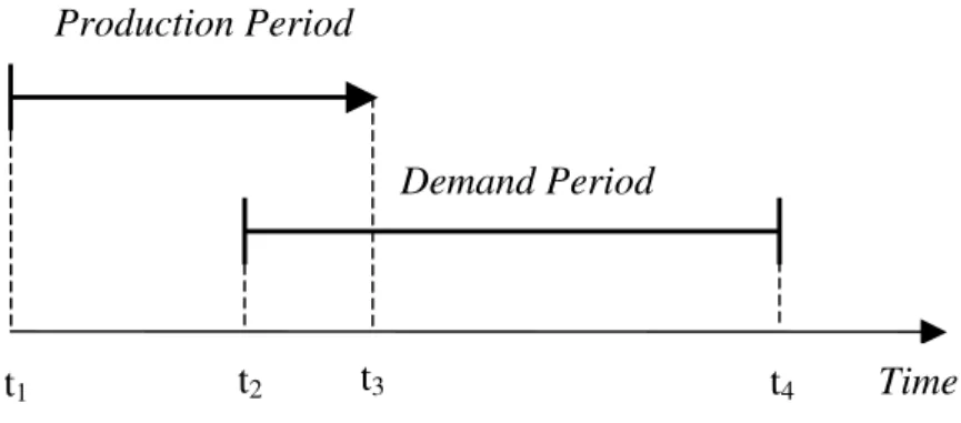
This research considers a decentralized two-stage supply chain consisting of a manufacturer and multiple retailers. The products that retailers order from the manufacturer are alike and require the same resources at the manufacturer's site. There is a single period of finite length, i.e. the demand period illustrated in Figure-1, during which random amounts of demand appear for the products. A retailer may have more than one product type to order. For the sake of generality, we use an index i (i=1, 2,...,N) to refer to a specific order, which is identified by its retailer and the product type jointly. The manufacturer announces the wholesale prices and the retailers decide on the optimal order quantities to maximize their expected profits. If the order quantity is not enough to satisfy the demand, then a retailer incurs a shortage cost per unsatisfied demand. If it is more than the demand, excess items are salvaged at a constant value per unit. The manufacturer has a finite production period, during which he/she has to produce the orders. Due to the limited production capacity, the manufacturer has the liberty of rejecting some orders. Transportation cost and time from the manufacturer to any of the retailers are negligible. Similarly, there is no cost or time spent by the manufacturer for production setups.

(19)

Figure 1: Production and Demand Periods (t1≤t2<t3<t4)

For this system, we propose a new contractual agreement that may increase manufacturers’ profits through a better utilization of his/her capacity. This is achieved by integration of the manufacturer's pricing and scheduling decisions. More specifically, the manufacturer offers a delivery time dependent wholesale price for each product type, which changes the retailers' ordering behavior in such a way that the manufacturer's production schedule is improved. We refer to this contract as delivery-date-dependent pricing (DTDP). We compare this type of contractual agreement to a more traditional one that we refer to as fixed wholesale

pricing with tardiness penalty (FWPT). As the name implies, in this contract, the

announced wholesale price by the manufacturer is constant regardless of the delivery time. If a delay occurs in the delivery time, a tardiness penalty is paid by the manufacturer at a predetermined rate per unit per unit time of delay.

Under these considerations, we next present a detailed description of the two contract types.

Contract FWPT:

• The manufacturer announces the wholesale prices before his/her production period begins. Wholesale prices are fixed and do not depend on order quantities or delivery times.

Production Period

t1 t2 t3 t4 Time

(20)

• Retailers decide on their optimal order quantities as if their orders will be delivered before the demand period begins.

• When all orders are received, the manufacturer accepts the ones that jointly maximize his/her profit under a limited production capacity.

• All accepted orders are quoted a delivery time of t₂. However, if an order

is delivered to its retailer after time t₂, $S _i per unit is paid by the

manufacturer for each unit time of delay.

It is important to note that, in this type of contract, the actual delivery time of an order may be different from the quoted delivery time. Furthermore, in case the manufacturer delays the delivery of an order, its quantity does not change and is given by the retailer's expected profit maximizer in period [t₂,t₄].

Contract DTDP:

• The manufacturer announces the wholesale prices before the production period, however different prices are quoted for different delivery times of an order.

• Each retailer evaluates the wholesale price, delivery time information and chooses a pair that maximizes his/her expected profits.

• Due to his/her limited production capacity, a manufacturer may again reject some of the orders.

• All accepted orders must be delivered no later than their quoted delivery times.

In the setting that is of interest in this paper, we assume that the manufacturer has full information about the demand process and the cost parameters of each retailer. Under this assumption, Contract DTDP allows the manufacturer to come up with a price schedule that implicitly forces a retailer to choose a wholesale

(21)

price, delivery time pair that increases the manufacturer's profits while keeping the

retailer satisfied. For modeling this type of a contract, we assume that there are 1

K+ different delivery dates that a manufacturer can quote to a retailer within the production period. We index the delivery dates by k (i.e., d_k) where k=0 refers to the start time of the manufacturer's production period. We assume that the demand for order i from time d _k to the end of the demand period has a

probability distribution with mean of k i

µ and standard deviation of k i

σ . Note that, in Contract FWPT , K =0 and d₀ = . t₂

In Contract DTDP, a retailer decides the delivery time of an order among a menu of wholesale price, delivery time pairs, and the manufacturer delivers an accepted order no later than that time. Therefore, a retailer who chooses a delivery date d k such that dk > , takes into account the expected demand lost until t2 dk,

and thereby, the new demand process with parameters k i

µ and k i

σ .

Before analyzing the manufacturer's and the retailers' expected profits resulting from the two contract types, we summarize below the notation introduced so far and that will be used throughout the paper.

i

r : Retail price per unit of Order i .

Q : Quantity of an order.

X : Random variable showing total demand at a retailer.

w : Wholesale price.

i

w : Market price for one unit of Order i .

( )

.

k i

f : Probability density function of demand for order i from time d k to

the end of the demand period.

( )

.

k i

F : Probability distribution function of demand for order i from time dk

(22)

(

w dij, ij

)

: A wholesale price, delivery time pair for the i

th_{retailer. Here, j is} the index of the pair.

i

b : Lost sale cost/unit of Order i .

i

g : Salvage value/unit of Order i .

i

h : Inventory cost of the manufacturer for holding one unit of Order i for a unit time.

i

S : Tardiness cost paid by the manufacturer for a unit time delay of Order i .

i

p : Manufacturer's processing time per unit of Order i .

i

c : Manufacturer's production cost per unit of Order i .

k

d : Value of delivery date k (d₀ = ). t₂

ϑ

: Contractual agreement type (FWPT or DTDP). C : Completion time of an order.

T : Length of the manufacturer's production period.

(

, ,

)

i Q w C

ϑ

∏ : Expected profits of the retailer for Order i in Contract

ϑ

.

(

, ,

)

i Q w C

ϑ

Ψ : Manufacturer's profits from Order i in Contract

ϑ

.

(

,

)

i Q C

ϑ

Θ : Tardiness penalty paid by the manufacturer for Order i in Contract

ϑ

.

The tardiness penalty paid by the manufacturer for Order i in Contract FWPT is

(

_,

)

(

2

)

eger 2 0 aksi taktirde i FWTP i C t S Q C t Q C  − ≥  Θ =      (1) Recall that in Contract DTDP, there is no tardiness cost. Therefore, we have

(

,

)

0

DTDP

i Q C

(23)

The expected profit of the retailer who places Order i is then given by

(

, ,

) (

)

k

(

)

(

) (

)

k

( )

(

,

)

i i i i i i i i i i Q Q w C r g w g Q r g b x Q f x dx Q C ϑ ϑ µ ∞ ∏ = − − − − − +

∫

− + Θ (3)

where k=arg min

{

k C: ≤d k_k, ∈

{

0,1,...,K

}

. The above expression is based on the following two assumptions: (i) the manufacturer delivers an order as soon as it is completed, (ii) the closest delivery time available larger than the planned completion time is quoted to the retailer. Notice that, these assumptions lead to the fact that, in Contract DTDP, the expectation of the retailer in terms of his/her profit for Order i is independent of the actual completion time as long as different completion times result in the same delivery date. That is, we have

(

, , 1

)

(

, , 2

)

DTDP DTDP

i Q w C i Q w C

∏ = ∏ , where dk−1<C1≤dk, dk−1<C2≤dk and

1 2

C ≠C . On the other hand, Contract FWPT implies that

(

, , 2

)

(

, , 1

)

FWTP FWTP

i Q w C i Q w C

∏ > ∏ for k ≥1. That is, under the assumption that the demand distribution does not change from C1 to C2, in Contract FWPT , the retailer is better off if his/her tardy-to-be order is delayed further. More specifically, depending on the lost sales cost and the value of tardiness cost, there may be cases where a retailer may increase his/her profits due to delayed orders.

The manufacturer's profit from Order i in both of the contracts is

(

, ,

)

(

)

(

1

)

(

,

)

2 i i i i i Q Q h p Q w C Q w c Q C ϑ + ϑ Ψ = − − − Θ (4)

The manufacturer's inventory holding cost, which is the second term of Expression (4), utilizes the fact his/her optimal sequence in both contract types is non-preemptive. Also, inventory holding costs start to accumulate for a product in Order i , at a rate of $h i per unit time, from the moment its processing begins until

the whole order is completed.

(24)

(

)

{ }

FWTP i 2 max , , s.t. Q 0 i Q w t Z+ Π ∈ ∪

where Z+_{denotes the set of positive integers. Note that the optimal quantity that} maximizes the expected profits of the retailer placing Order i (i.e., Qi

∗ _{) is given} by

{ }

0

( )

min 0 i i i i i i i i r w b Q Q Z F Q r g b ∗  + − +  =  ∈ ∪ ≥  − +   (5) In Contract DTDP, the retailer of Order i is offered a menu of delivery dates with corresponding wholesale prices, and he/she chooses the pair that maximizes his/her expected profits as follows:

(

)

{ }

DTDP i max , , s.t. Q 0 , ij ij Q w d Z+ j Π ∈ ∪ ∀

In both of the contractual agreements, after the manufacturer receives the optimal order quantities for all orders, he/she prepares the production schedule. Due to his/her limited production capacity, the manufacturer may reject some of the orders. Recall that, in contract DT DP, the manufacturer offers a delivery time dependent price schedule before the orders are collected. This gives the manufacturer the opportunity to consider beforehand his/her scheduling decisions simultaneously with pricing decisions, and thereby, to increase his/her profits under limited capacity. In using pricing as a mechanism to change the ordering behaviors of the retailers, the manufacturer should put the expected profits of the accepted retailers no worse than what they would be under the market price with a delivery time t₂. That is, the expected profit for Order i , if it is accepted under

Contract DTDP, should at least be equal to FWTP

(

, , ₂

)

i Q w ti i

∗

∏ . Otherwise, the

retailer who owns Order i may reject the business of the current manufacturer and may find alternative suppliers in the market. For a single order, there may be

(25)

several wholesale price, delivery date pairs (i.e.,

(

w dij, ij

)

) that put the retailer's

expected profits no worse than FWTP

(

, , ₂

)

i Q w ti i

∗

∏ . Considering all such pairs over all orders, the manufacturer should choose a pair for each order such that when all retailers demand the optimal order quantities under those pairs, the manufacturer achieves the maximum profit under limited production capacity. Finally, the manufacturer prepares a menu of prices and delivery dates for each order. In order to model the manufacturer's perspective in Contract DTDP, we will follow the below steps:

I. Finding

(

w d_ij, _ij

)

pairs that put the retailer's expected profits no worse than

(

, , 2

)

FWTP

i Q w ti i

∗

∏ for each Order i . The vector of all such pairs for Order i will be denoted by J_i.This step will be referred to as Preparation of Wholesale Prices and Delivery Dates.

II. Among Ji number of pairs for Order i , finding the one those results in

the maximum profit for the manufacturer with other orders, for all i . This step will be referred to as Preparation of the Price Menu.

(26)

C h a p t e r 4

Manufacturer's Subproblem in Contract

DTDP

4.1 Preparation of Wholesale prices and Delivery Times

In this section, we present a search algorithm to identify

(

w d_ij, _ij

)

pairs that put the retailer's expected profits no worse than FWTP

(

, , ₂

)

i Q w ti i

∗

∏ for each Order i . This search algorithm will utilize the following proposition and the remark.

Proposition 1: Let Q₁ and Q₂ be two order quantities that maximize the

expected profits or a retailer for Order i for a given delivery date d_k at wholesale

prices w₁ and w₂, respectively. That is, Q₁ satisfies k

( )

₁ i 1 i i i i i r w b F Q r g b − + = − + and Q2 satisfies

( )

2 2 k i i i i i i r w b F Q r g b − + = − + . If Q2 >Q1, then we have DTDP

₍

₂, ₂,

₎

DTDP

₍

₁, ,₁

₎

,

_{

0,1,...,

_}

i Q w dk i Q w dk k K ∏ > ∏ ∀ ∈

Proof: Using Expression (3), we have

(

) (

)

(

)

(

) (

)

( )

1 1, 1, 1 1 1 DTDP k k i k i i i i i i i i Q Q w d r g

µ

w g Q r g b x Q f x dx ∞ ∏ = − − − − − +

∫

− (6) and

(27)

(

) (

)

(

)

(

) (

)

( )

2 2, 2, 2 2 2 DTDP k k i k i i i i i i i i Q Q w d r g

µ

w g Q r g b x Q f x dx ∞ ∏ = − − − − − +

∫

− (7) Plugging in 1

(

)

( )

1 k i i i i i i w = +r b − r −g +b F Q and

(

)

( )

2 2 k i i i i i i

w = +r b − r −g +b F Q in Expressions (6) and (7), respectively, we have

(

) (

)

(

)

( )

1 1, 1, DTDP k k i k i i i i i i i Q Q w d r g

µ

r g b xf x dx ∞ ∏ = − − − +

∫

and

(

) (

)

(

)

( )

2 2, 2, DTDP k k i k i i i i i i i Q Q w d r g

µ

r g b xf x dx ∞ ∏ = − − − +

∫

Since Q₂ >Q₁, using the above two equations, it follows that

(

2, 2,

)

(

1, 1,

)

DTDP DTDP

i Q w dk i Q w dk

∏ > ∏

In order to form J _i for each Order i , we propose an algorithm that is based on a

search procedure over Q for a given d _k over all k∈

{

1, 2,...,K

}

. Algorithm I:

(A1) Start with the first delivery date (i.e., t₂) and set the index of the first pair

to zero. That is, k=0 and j= . 0

(A2) For the current delivery date d_k, using Algorithm 2, find the smallest

integer Q such that

(

, ,

)

₍

, , 2

₎

DTDP FWTP i Q w dk i Q w ti i ∗ ∏ ≥ ∏ where

(

)

k

( )

i i i i i i

w= +r b − r −g +b F Q . If none exists, go to Step (A4). Otherwise, set

(

w d_ij, _ij

)

=

(

w d, _k

)

, FWTP

₍

, ,

₎

i k

m= Ψ Q w d and j= + . j 1

(A3) Increase Q one by one and find the wholesale price at which Q is optimal, until the wholesale price falls below c_i. Add new pairs for quantities that

(28)

1. Set Q = Q + 1. 2. Set

(

)

k

( )

i i i i i i w= +r b − r −g +b F Q . 3. If w≤c_i, go to Step (A4). 4. If FWTP

₍

, ,

₎

i Q w dk m Ψ > , set

(

w dij, ij

)

=

₍

w d, k

₎

,

(

, ,

)

FWTP i k m= Ψ Q w d and 1 j= + . Go to Step (A3).1. j

(A4) Proceed with the next available delivery date. If there is none, stop the algorithm. That is,

1. If k<K, set k= +k 1 and go to Step (A2).

2. Else, set J_i = and stop the algorithm returning j J . _i

Algorithm II:

(B1) If k= , stop and return 0 Q=Q_i∗.

(B2) Compute the retailer's optimum order quantity at the market price assuming that the order is quoted a delivery date of d_k. That is, find the minimum

integer Q such that k

( )

i i i i i i i r w b F Q r g b − + ≥ − + . If

(

, ,

)

(

, , 2

)

DTDP FWTP i Q w di k i Q w ti i ∗ ∏ ≥ ∏ ,

go to Step (B3). Else, go to Step (B4).

(B3) Decrease Q one by one until

(

, ,

)

₍

, , 2

₎

DTDP FWTP i Q w dk i Q w ti i ∗ ∏ < ∏ where

(

)

k

( )

i i i i i i w= +r b − r −g +b F Q , or Q= . If 1 DTDP

(

, ,

)

FWTP

(

, , ₂

)

i Q w dk i Q w ti i ∗ ∏ < ∏

is reached first, stop and return Q+ . If 1 Q= is reached first, stop and return Q . 1 (B4) Increase Q one by one until DTDP

₍

, ,

₎

FWTP

(

, , ₂

)

i Q w dk i Q w ti i ∗ ∏ ≥ ∏ or i w<c where

(

)

k

( )

i i i i i i w= +r b − r −g +b F Q . If

(

, ,

)

₍

, , 2

₎

DTDP FWTP i Q w dk i Q w ti i ∗

∏ ≥ ∏ is reached first, stop and return Q . If w<c_i

(29)

Algorithm I in conjunction with Algorithm II, provides the set J for a given _i

order. Notice that, a wholesale price, delivery date pair within this set result in an expected profit of at least FWTP

(

, , ₂

)

i Qi w ti

∗

∏ . Therefore, we assume any pair in this set is acceptable by the retailer of Order i . After the manufacturer finds all such pairs for all orders by running Algorithm I for i=1, 2,...,N, he/she prepares the production schedule. In the next section, we present a model for the manufacturer to decide which orders he/she will accept, and what wholesale price and delivery date he/she will quote for accepted orders, while preparing his/her production schedule.

4.2 Preparation of Price Menu

In the previous section, we presented an algorithm for the manufacturer to find wholesale price values paired with delivery dates for an Order i , which put the ordering retailer in a no worse expected profits than FWTP

(

, , ₂

)

i Qi w ti

∗

∏ . Next, we

present an optimization model for the manufacturer to decide which orders to accept/reject, and the best wholesale price, delivery date pair for each accepted order that maximizes his/her expected profits under limited production capacity.

The decision variables in this optimization model are as follows: 1 if pair is chosen for Order

0 otherwise th ij j i y =   

1 if Order , for which pair is chosen, is scheduled before Order , for which pair is chosen

0 otherwise th th ijlm i j x i m     =     

1 if Order for which pair is chosen, is completed after 0 otherwise th ij ij i j d α =     

(30)

ij

C : Production finish time of production of Order i for jth pair

The mathematical model presented below can be used to make the scheduling and order acceptance/rejection decisions in both contractual agreements. More specifically, for Contract DTDP, S _i is set to a very large number, and set J _i

formed according to Algorithm I, is used for each order. For Contract FWPT, S _i is

set to its value as it is determined by the manufacturer, and J _i only includes

(w ti, ₂).

Before proceeding with the mathematical model, we define one more notation. Let k be the index of delivery date dij . For pair (wij ,dij ), we define Qij as

follows:

{ }

( )

min 0 k i ij i ij i i i i r w b Q Q Z F Q r g b +  − +    =  ∈ ∪ ≥  − +    

If the following model results in yij =0 for all pairs j in set Ji, this implies

that Order i is rejected. Otherwise, it is accepted.

MODEL I : Objective Function

(

)

(

)

(

)

1 0 1 0 1 0 1 max 2 J J N N ij i i ij ij ij ij ij i i j i j J N ij ij ij ij ij i i j i i i y p h Q Q y Q w c y α C d Q S = = = = = = + − − − −

∑∑

(8) Constraints

Don’t exceed the total capacity

1 0 J N ij i ij i j i Q p y T = = ≤

∑∑

(9) Determine a wholesale price for accepted orders

(31)

0 1 for all J ij j i y i = ≤

∑

(10) Precedence relationships and capacity allocations

( )

(

)

( ) (

)

xijlm+xlmij=1 for all i, j ve ,l m such that ,i j ≠ l m, (11)

(

)

( )

(

)

( ) (

)

1 for all ve , such that , , lm ij lm l ijlm ijlm C C Q p x x M i, j l m i j l m − ≥ − − ≠ (12) Orders cannot be completed at time zero

( )

for all

ij ij i

C ≥Q p i, j (13) Determine tardiness amounts

( )

for all

ij ij ij

C −d ≤

α

M i, j (14) Define range of decision variables

{ }

0 1 for all

( )

ve ,

(

)

such that

ijlm x ∈ , i, j l m i l≠ (15)

{ }

0 1 for all

( )

ij y ∈ , i, j (16)

{ }

0 1 for all

( )

ij , i, j

α

∈ (17) The objective function in the above model includes the manufacturer's revenue from sales, inventory holding costs and tardiness costs for all orders that are accepted. Expression (9) guarantees that production capacity is not exceeded. Expression (10) ensures that if an order is accepted, a single wholesale price,

delivery date pair is chosen for this order. Expressions (11) and (12) jointly

determine the precedence relationships. Expression (13) eliminates zero completion times. Expression (14) determines which orders are tardy. Finally, Expressions (15), (16) and (17) define the range of decision variables.

It can be observed that the objective function in MODEL I is nonlinear.

MODEL II that will be presented next, builds upon MODEL I and is linear. An

additional decision variable that will be referred to as

υ

ij will be used in this

(32)

ij

υ

: Tardiness amount for Order i if jthpair is chosen for this order.

MODEL II : Objective Function

(

)

(

)

1 0 1 0 1 0 1 max 2 J J N N ij i i ij ij ij ij ij i i j i j J N ij i ij i j i i i y p h Q Q y Q w c Q Sν = = = = = = + − − −

∑∑

(18) Constraints

Don’t exceed the total capacity

1 0 J N ij i ij i j i Q p y T = = ≤

∑∑

(19) Determine a wholesale price for accepted orders

0 1 for all J ij j i y i = ≤

∑

(20) Precedence relationships and capacity allocations

( )

(

)

( ) (

)

xijlm+xlmij=1 for all i, j ve ,l m such that ,i j ≠ l m, (21)

(

)

( )

(

)

( ) (

)

1 for all and ,

such that , , lm ij lm l ijlm ijlm C C Q p x x M i, j l m i j l m − ≥ − − ≠ (22) Orders cannot be completed at time zero

( )

for all

ij ij i

C ≥Q p i, j (23) Determine tardiness amounts

( )

for all ij y M ij i, j

ν

≤ (24)

(

1

)

for all

( )

ij Cij dij y M ij i, j

ν

≥ − − − (25) Define range of decision variables

( )

0 for all

ij i, j

ν

≥ (26)

{ }

0 1 for all

( )

ve ,

(

)

öyleki

ijlm

(33)

{ }

0 1 for all

( )

ij

y ∈ , i, j (28) The objective function in the above model includes the manufacturer's revenue from sales, inventory holding costs and tardiness costs for all orders that are accepted. Expression (19) guarantees that production capacity is not exceeded. Expression (20) ensures that if an order is accepted, a single wholesale price,

delivery date pair is chosen for this order. Expressions (21) and (22) jointly

determine the precedence relationships. Expression (23) eliminates zero completion times. Expression (24) and (25) determine which orders are tardy. Finally, Expressions (26), (27) and (28) define the range of decision variables.

We realize that, after some initial runs of MODEL-I for Contract DTDP even for identical retailers, this formulation permits us to solve small-scale problems. Fortunately, by reducing the number of variables we solve sufficiently large-scales optimization problems for identical retailers. To achieve this, we use the following two facts: (1) the sequence of production orders for a given latest delivery time does not change the total expected profit of the manufacturer as long as they are consecutively produced and (2) the process should be non-preemptive whenever the production of an order starts. For example, consider two delivery times and suppose half of the orders are promised to be shipped until first delivery time and the rest is until the second one. Furthermore, the manufacturer uses all its production capacity. All non-preemptive sequences ensuring that all orders are shipped prior their promised times result in same profit for the manufacturer. Notice that first fact follows from the fact that there is no tardiness cost in Contract DTDP.

Basically, the optimization model decides which orders are selected at what wholesale prices for each delivery times. The model achieves this by ensuring that for a given delivery time total used capacity does not exceed actual capacity and there is no late delivery until that time. Similar to previous models, new model

(34)

maximizes the total profit. For this model, we need to, in addition to previous notation, define the following parameters and decision variables.

Parameter

k

TC : Total actual capacity until kth delivery time

Decision variable

1 if order at price is selected to be shipped until delivery time 0 otherwise th th ijk i j x k     =      MODEL III Objective Function

(

)

1 0 0 1 0 0 ( 1) max 2 i i J J N K N K ijk i i ij ij ijk ij i ij i j k i j k x p h Q Q x w c Q = = = = = = + − −

∑∑∑

(29) Constraints

If order accepted, determine a single price and delivery time

0 0 1 for all i J _K ijk j k x i = = ≤

∑∑

(30) Do not exceed the capacity

1 0 for all i J N ijk i ij k i j x p Q TC k = = ≤

∑∑

(31) Define range of variables

{ }

0 1 for all

(

)

ijk

x ∈ , i, j,k (32) The objective function in the above model includes the manufacturer's revenue from sales, and inventory holding costs for all orders that are accepted. Expression (30) ensures that if an order is accepted, a single wholesale price,

(35)

capacity until each due-date is not exceeded. Finally, Expression (32) defines binary variables.

(36)

C h a p t e r 5

EXPERIMENTAL DESIGN AND

NUMERICAL RESULTS

In this section, we numerically compare Contract DTDP with Contract FWTP. We consider homogeneous retailers in the sense that their ordering system and its parameters, introduced and defined as in the previous chapter, are identical. In the experiments, we characterize different market settings and determine which contract type provides better performance under which scenarios. The numerical results are interpreted as managerial insights, which should provide useful guidance for pricing and production-scheduling decisions in various supply chain settings.

5.1 Experimental Design

We consider six homogeneous retailers. Each retailer gives an order and all orders are for a single product. Retailer i has a Normal demand with a mean of

µ

i

and a standard deviation of

σ

_i, for i=1, 2,..., 6. The length of the demand period is set t₄−t₂ =2000 (see Figure-1). We use Normal demand in order to make the numerical analysis simple. More specifically, we exploit the fact that the sum of Normal random variables is Normal. Unit retailer price and wholesale price of the product in the market are r_i =1 and wi =0.75, respectively. Retailers are not

(37)

subject to any salvage and backlog costs (i.e. b_i =0, g_i =0, i=1,...,6). The

production period is set half as long as the demand period (i.e. t3−t1 =1000).

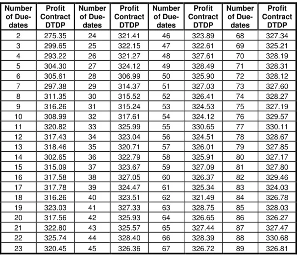
Recall that Contract DTDP requires the number of due dates to be set as an endogenous variable, Preliminary experimentation indicates that this variable may have a considerable effect on the profit obtained by the manufacturer under Contract DTDP. Note that no such effect is present for Contract FWTP as it contains a single due date which is the beginning of the demand period. In the case of Contract DTDP, on the other hand, it is crucially important to set the number of due dates in accordance with the total production capacity in the

demand period. This is mainly due to the fact that the manufacturer applies

discounted wholesale prices for the orders whose due dates are in the demand

period and there will be loss in profits for the manufacturer if there are time gaps

between due dates and production completion times. In other words, if the manufacturer ships the orders exactly at their due dates, then discounts will be less and hence, the profits of the manufacturer will be larger. As a result, the profitability of the manufacturer increases with the number of due dates under Contract DTDP.

Some preliminary experimentation indicates that the number of available due dates to ensure better performance of Contract DTDP increases with the order size and the number of orders to be shipped within the demand period,. In our experimental setting, the largest order size is 97 and we can ship at most six orders within the demand period. Consequently, we use 582 capacity units (set as six times the size of the largest order) to graphically illustrate this effect in Figure 2 (Data is given in Appendix-C). The figure indicates that profitability shows some improvement as the number of due dates increases up to a certain point and stabilizes thereafter. Based on preliminary results under different settings, we fix the number of due dates at 80 in the remainder of our experimentation.

(38)

270 280 290 300 310 320 330 340 0 10 20 30 40 50 60 70 80 90

Number of Due Dates

P ro fi t in C o n tr a c t D T D P

Figure-2: Profitability of Contract DTDP as a function of the number of due dates We vary several factors and compare the performance of the two contract types. On the retailer side, the only factor that we manipulate is the stochasticity of demand. On the manufacturer side, we focus on production capacity before and after the beginning of the demand period, as well as the production, inventory and tardiness costs.

Stochasticity is measured by the coefficient of variation defined as

i i i

CV =

σ µ

for retailer i. CVi directly affects the optimal order sizes, which are given by

(

( )

k 1

₍

1

₎

1

)

i i i i i

Q∗₌µ CV _× F − ₋w ₊ _{. In Contract DTDP, optimal order sizes}

to be shipped within the demand period are affected by two issues: (1) loss of the demand between the due date and time of order fulfillment (2) discounts offered by the manufacturer. In the equation above, an optimal order size is determined as the sum of two terms. Stochasticity only affects the first one of these terms and it is independent of the aforementioned two issues affecting the optimal order size. This allows us to analyze the effect of stochasticity while fixing all decisions.

(39)

Our focus is to numerically analyze our proposal in different levels of stochasticity and in the experimentation, we use two levels for CV_i which are

0.05 and 0.3 and a fixed mean value of µi =100.

Assuming that the production capacity is uniform throughout the production period, it is helpful to consider the production period as of two parts before and after the beginning of the demand period. These two parts are of length

(

t2−t1

)

and

₍

t₃−t₂

₎

, respectively. We vary the capacity prior to the beginning of the

demand period by varying

t

2

−

t

1 between 1 to 585 units. This factor is important

in that if

(

t2−t1

)

is long enough to produce all orders, then the two contract types will perform equally well in terms of the manufacturer’s profit. Thus, we would like to illustrate the effect of capacity in

(

t2−t1

)

by considering various levels of this factor. For t₃− or capacity during the demand period, we use four levels, t₂

selected as 140, 280, 420 and 585.

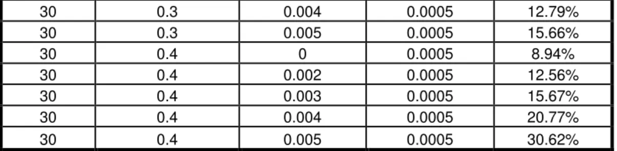
Production and inventory costs are two important factors affecting manufacturer’s production decisions and the relative performance of the two contract types. We consider the following five levels for the production cost: 0, 0.1, 0.2, 0.3 and 0.4. Similarly, we use five levels also for the inventory cost, which are set at 0, 0.002, 0.003, 0.004 and 0.005. For any given production and inventory cost combination, we select appropriate market and wholesale prices so that the resulting manufacturer’s profit is positive. The values used for this factor is determined in a way that the manufacturer has some positive profit. Otherwise, the manufacturer would not prefer to process any order.

Tardiness cost is only included in contract FWTP. It affects the total profits

and the number of orders accepted to be processed in contract FWTP. For instance, if it is high enough, there will be no order committed to be shipped during the demand period. We use the values of 0.0001, 0.0002, 0.0003, 0.0004

(40)

and 0.0005 as five alternative levels of this factor. To assess the feasibility of this choice, we focus on the highest possible tardiness penalty, which occurs when the selected order is shipped at the end of the production period. Similar to the previous factor, the manufacturer has incentive to make production under these levels for this factor. Thus, our numbers are feasible under this setting.. The tardiness values can also be interpreted as a measure of the relative strength of the two parties in the trade. If the tardiness cost is high, retailers are more influential. Otherwise, the manufacturer has virtually no competition and hence can govern the terms.

5.2 Numerical Results

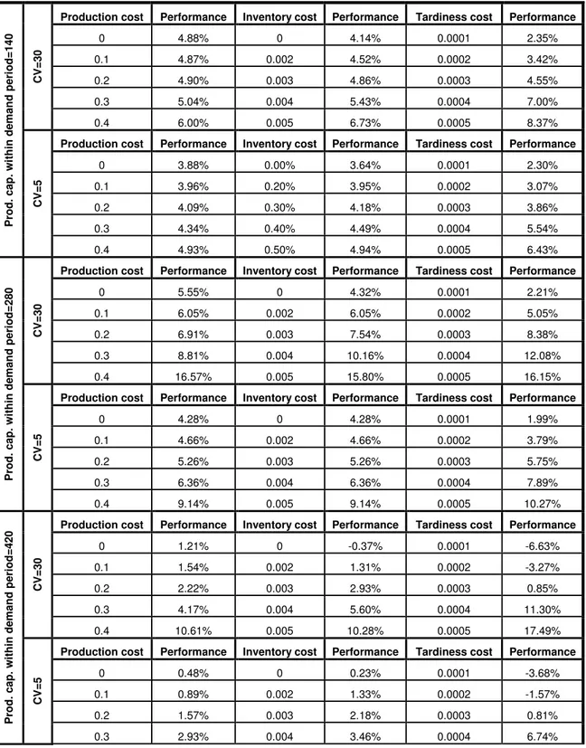
In this section, we present the experimental results in terms of the percentage difference of the performance of Contract DTDP over that of Contract FWTP . We consider one factor at a time and use average percentage difference in the graphs. The performance measure is mathematically defined by the following expression.

(

)

(

)

(

)

(

)

6 6 1 1 100 DTDP , , FWTP , , FWTP , , i i i i i Q w C Q w C Q w C = = ×

∑

Ψ − Ψ

∑

Ψ

The raw data to illustrate the comparison between the two contracts is also given in Appendix-A. In addition, the summary of average performance for each factor is included in Appendix-B.

In what follows, we first discuss the effects of production, inventory and tardiness costs. Then we proceed with analyses of the effect imposed by the portion of the production period residing within the demand period. We conclude our experimental investigation with observations on the impact of the degree of stochasticty of retailer demand on the relative performance of the two contracts.

The Effect of Production Cost: Figure-3 depicts the average percentage performance of Contract DTDP over contract FWTP for five different values of production cost. The results indicate that Contract DTDP becomes more

(41)

preferable as the production cost increases in the market. More specifically, if the cost is 0.4, then the relative performance is around 38%, which means that Contract DTDP generates 38% more profit relative to Contract FWTP. Interestingly, Contract DTDP is still more preferable even if there is no production cost at all. This observation may be important also in that it once again emphasizes the value of information sharing in supply chain settings.

0.00% 5.00% 10.00% 15.00% 20.00% 25.00% 30.00% 35.00% 40.00% P e rc e n ta g e d if fe re n c e i n p e rf o rm a n c e 0 0.1 0.2 0.3 0.4 Production cost

Figure-3: The effect of production cost on the performance of DTDP relative to that of FWTP

The Effect of Inventory Cost: Figure-4 illustrates the effect of inventory cost on the relative performance of DTDP. In parallel with the effect of the production cost, Contract DTDP generates more profit than Contract FWTP and this difference becomes more marked for increasing values of the inventory cost. This observation can be explained based on the formulation of the two contracts. In both contracts, inventory cost per order is proportional to the square of the order size. We know that order sizes in Contract DTDP decreases if the order is committed to be shipped within the demand period. This is simply because it

Coordination of pricing and production-scheduling decisions in supply chains