Received 12 March 2014, Revised 1 July 2014, Accepted 8 July 2014 Published online 12 August 2014 in Wiley Online Library
(wileyonlinelibrary.com) DOI: 10.1002/asmb.2058
The impact of price skimming on supply and
exit decisions
Ay¸segül Toptal
a*†and Sıla Çetinkaya
bStochastic inventory control theory has focused on the order and/or pricing policy when the length of the selling period is known. In contrast to this focus, we examine the optimal length of the selling period—which we refer to as market exit time—in the context of a novel inventory replenishment problem faced by a supplier of a new, trendy, and relatively expensive product with a short life cycle. An important characteristic of the problem is that the supplier applies a price skimming strategy over time and the demand is modeled as a nonhomogeneous Poisson process with an intensity that is dependent on time. The supplier’s problems of finding the optimal order quantity and market exit time, with the objective of maximizing expected profit, is studied. Procedures are proposed for joint optimization of the objective function with respect to the order quantity and the market exit time. Then, the effects of the order quantity and market exit time on the supplier’s profitability are explored on the basis of a quantitative investigation. Copyright © 2014 John Wiley & Sons, Ltd.
Keywords: price skimming; market exit; end of life; nonhomogenous Poisson process
1. Introduction and related literature
We consider a new, trendy, and relatively expensive product that has a limited supply and a short life cycle associated with its fast-clockspeed industry. Hence, it is in the market for a short selling period. Examples of interest include high-end/designer clothing, accessories, perfumes, cosmetics, jewelery, toys or so-called status or fad items that go in and out of fashion, and some electronics or technology products that become obsolete as newer and better products are introduced. Because of the short life cycle, there is only a single replenishment opportunity for the supplier at the beginning of the selling period. Therefore, given the pricing strategy, we are concerned with (i) the order quantity and (ii) the length of the selling period, which we refer to as market exit time, taking the perspective of the supplier of the product.
The supplier in consideration is the new product’s inventor and has significant sunk costs associated with development. There are no competitors in the market currently; however, the competition may eventually step in with imitations or product substitutes. The inventing supplier desires and estimates to be out of the market by that time. In this setting, the market can be divided into distinct segments according to the customers’ willingness to pay. In order to recoup development-related sunk costs, the supplier initially targets the segment that is willing to pay the highest price. This group of customers includes early adopters who are relatively insensitive to price. Over time, the supplier sequentially reduces the price for the next customer segment aiming for shoppers who are more price sensitive and have not purchased the product yet.
This form of pricing strategy is referred to as ‘price skimming’ in the marketing literature [1, 2] and is used for differ-ential pricing in cases of heterogenous consumer segments depending on their willingness to pay. By reducing the prices systematically over time, the supplier skims the revenues layer by layer from the market. Apple, Du Pont, Polaroid, and Sony are known to have used skimming to benefit from high, short-term profits for their innovative products. Pharmaceuti-cal companies also apply price skimming to fund their research and development activities before the generic alternatives eventually decrease the prices [3].
Skimming is a strategy for new product pricing, and it is common for ‘status’ or ‘fad’ items. It is also known as periodic
discounting or riding down the demand curve [1]. Price skimming is most appropriate when [4, 5]
aIndustrial Engineering Department, Bilkent University, Ankara, 06800, Turkey
bIndustrial and Systems Engineering Department, Texas A&M University, College Station, TX 77843-3131, U.S.A.
*Correspondence to: Ay¸segül Toptal, Industrial Engineering Department, Bilkent University, Ankara, 06800, Turkey.
†E-mail: [email protected]
• the high price is perceived as a sign of high quality,
• there are enough customers willing to purchase the product at high prices, • the cost of producing small volumes is relatively low, and
• competitors cannot enter the market quickly because of protection by patents, secrets of production, or by other barriers.
These conditions are particularly applicable for various status or fad items. Penetration pricing and experience curve pricing are the other ways to price new (perhaps, more lasting) products [2].
Tellis [1] reports that when a price skimming strategy is in place, the manner of discounting is predictable over time, and it is not necessarily unknown to consumers. Hence, we also consider the case that the supplier has effectively segmented the market, knows the highest price payable by the consumers in each segment, and has a well-defined pricing strategy to decrease prices over time. Further, we assume that customers behave myopically, an assumption that is especially applicable to buyers of status or fad items. That is, they do not develop strategies against the supplier and wait to purchase the item the first time the current price drops below their valuation [6]. In fact, because of the circumstances that price skimming is applied and the status or fad nature of the product, early adopters are not deterred from buying the product at high prices even if they know the prices will be lowered later. On the contrary, status-conscious, early adopters help the supplier drive the perception of the brand, so the supplier continues to attract more elastic segments of the market over time, even if the competition is expected to enter the market at lower prices.
In broad terms, the underlying integrated inventory/marketing problem is motivated and characterized by the following three key issues that, in turn, differentiate the paper’s setting of interest from that of more traditional settings:
1. The product’s price is initially set to a high value and then systematically reduced over time under price skimming, that is, the pricing strategy of the supplier is modeled using a linearly decreasing function of time. Assuming a finite population and customers’ valuations are uniformly distributed at a certain interval, it has been shown that the structure of the optimal price skimming strategy is in fact linearly decreasing in time [7, Chapter 5]. Many studies on dynamic pricing also allow prices to change continuously over time (e.g., [8, 9]). Clearly, changing prices continuously is most appropriate when relabeling costs are negligible, and these costs have been dropping in many applications, because of the growing Internet-based sales systems [10, 11].
2. Because of the nature of the product (e.g., status or fad item) and the pricing strategy in place, the market demand has an intensity that is dependent on time, and indirectly on the price, that is, the demand arrival process at the supplier is characterized by a nonhomogeneous Poisson (NP) process to represent time-dependent nature of the demand. Note that, because the price is exogenous, we do not explicitly model the dependency between price and demand. However, the linear structure of the time-varying demand intensity implicitly incorporates those cases in which demand intensity is a linearly decreasing function of price. Bitran and Mondschein [12] and Zhao and Zheng [13] also model customer arrivals according to an NP process with general intensity in different problem settings.
3. The cost is high for holding one unit of the product in inventory for a unit time due to high initial market value and price depreciation over time. That is, although we are faced with a single-period inventory problem—in the sense that there is a single replenishment opportunity—holding costs are modeled carefully while keeping track of inventory depletion times. In other words, tracking the demand arrivals in a continuous fashion allows us to model holding costs precisely. This approach is critical because of the nature of the product in consideration.
Consequently, inventory-related costs build up substantially for unsold items as time evolves, and the corresponding order quantity and market exit time decisions should be examined carefully for profitability. For this purpose, first we develop an analytical expression of the supplier’s expected profit function in which decreasing prices, changing demand over time, and holding costs are modeled explicitly. Then, we investigate the effects of the order quantity and market exit time on the supplier’s profitability based on analytical and numerical investigations. We also propose procedures for the supplier’s joint decisions for order quantity and market exit time to maximize his or her expected profits.
Because our modeling of demand intensity implicitly incorporates price sensitivity as discussed earlier, our work is also related to joint ordering/production and pricing literature (e.g., [9, 14–20]). This line of literature generally assumes the demand is simply price sensitive, so the dependency between demand and price is modeled using the function𝛼tD(pt) +𝛽t where𝛼tand𝛽t are random variables and D(pt) is a decreasing function of price pt in period t. Note that additive (e.g., [21]) and multiplicative demand (e.g., [22]) cases are special forms of this more general function [23, 24]. However, our focus is on time-dependent demand rather than price sensitivity. By modeling the demand arrivals as an NP process and allowing the intensity to be increasing or nonincreasing, we incorporate the natural decrease in customers’ willingness to purchase the item in time as well as the market broadened by decreased prices.
While analyzing the ordering and market exit time decisions for a new product subject to price skimming, our objective is to answer the following questions:
Q1. If the supplier plans to stay in the market for a limited duration, what is the desirable order quantity for generating a profit under explicit sunk costs?
Q2. For a given level of initial inventory, what is the optimal market exit time?
Q3. How does the supplier’s expected profit and the optimum market exit time change for varying levels of demand sensitivity with respect to price?
Q4. How does the supplier make joint decisions for market exit time and replenishment quantity?
However, the proposed model also has potential to be useful for making decisions regarding an end-of-life product. In fast-clockspeed industries, because of rapid changes in technology and fashion, inventory is liquidated via planned price reductions over time. The end-of-life products in these industries either are displaced with the introduction of a new product as in the context of product rollovers [25–29] or are fad items that simply disappear from the market with no replacement. Whether there is a replacement product or not, it is important to make careful manufacturing and business decisions for phasing out an end-of-life product, as the related costs may be significant. For example, Hewlett Packard Company reports more than $20m annual end-of-life-cycle write-off expenses for the computer servers division [30]. The end-of-life prod-uct’s final order quantity [31], on-hand inventory, salvage value, pricing strategy, and demand process are among the issues that need to be considered for planning a product’s phase-out.
Recall that examples for the products of interest in this paper include fad, status items that go in and out of fashion quickly (e.g., high-end/designer clothing, accessories, perfumes, cosmetics, jewelery, and toys) and some electronic prod-ucts that become obsolete because of improved technology or competition. It is worth noting that some of these prodprod-ucts are ‘personal-taste items’, which simply disappear from the market with no true replacement, for example, fad clothing items such as Valentino designer leggings priced at $990, and currently in-stock, at Saks Fifth Avenue. Others, for exam-ple, some electronic toys or games, face competition eventually with imitations or perhaps substitutes. Our main focus is on the former class of products under the assumption that the supplier in consideration is the inventor of the product with no competitors in the market currently. Although the competition may eventually step in, the inventing supplier predicts to go out of the market by that time, so we do not explicitly consider a replacement/new product. However, we do propose a useful way of examining the impact of delayed market exit time (or product rollover if there is a replacement) on profits.
That is, we do not specifically account for a new product or an improved generation of the same product that will be sold in the market after the current product is discontinued. By including the marginal profit of the new product into the lost-sale cost per unit of the current product, we can address the opportunity cost of losing the new product’s profit when it is not yet introduced and the old product runs out of stock before the planned market exit time. Hence, our model is also potentially useful for answering the following managerial questions, which are related to liquidation of an end-of-life product:
Q5. What should be the order quantity in the last replenishment of an end-of-life-cycle product for which market exit time is known?
Q6. What is the maximum order quantity for a soon-to-be-discontinued product to generate some positive profits? Q7. What is the impact of delaying market exit time (or product rollover if there is a replacement) on profits? Q8. How do the market exit times differ for varying levels of demand sensitivity to decreasing prices? Q9. How should the price skimming decisions be made for an end-of-life product, given the market exit time?
The remainder of the paper is organized as follows. In Section 2, we discuss our assumptions and present the general model. In Section 3, we develop the supplier’s expected profit function for the nonhomogenous demand intensity. A detailed analysis of the special case with Poisson demand arrivals follows in Section 4. In Section 5, we present our results on the general case. Finally, in Section 6, we summarize our fundamental results and answers to the aforementioned questions (Q1–Q9).
2. Problem definition and notation
We consider a supplier who faces random demand during a finite horizon of length T. The supplier has a single replen-ishment opportunity at the beginning of the demand period. If the quantity produced is less than the demand, the supplier incurs a penalty of $b∕unit. Items unsold at the end of the period are salvaged with a per unit earning of $v∕unit. Each item that stays in the supplier’s inventory brings a cost of $h∕unit∕unittime. The supplier incurs $c for each unit manu-factured and an additional amount of $K as a fixed replenishment/development cost. Because the proposed model can be applied to the different stages in the life cycle of a product, the fixed cost K may be due to ‘replenishment’ or ‘develop-ment’ depending on the context. For example, if the model is used to decide the order quantity in the last replenishment of an end-of-life-cycle product, K would strictly refer to the fixed cost of replenishment.
As discussed in Section 1, the supplier has planned reductions of the price over time representing the price skimming strategy of interest [1, 2, 4]. More specifically, the price of an item at time t, that is, r(t), is given by𝛼 − 𝛽t. Also, as we noted earlier, the demand arrival process at the supplier is characterized by an NP process whose intensity is given by
𝜆0+𝜆1t where𝜆0⩾ 0. Under a price skimming strategy—depending on the size of the market in each customer segment,
or under a liquidation policy—depending on how the increase in demand due to the decreasing price compares with its natural decrease, we further consider the following three cases:
• 𝜆1 > 0: This happens when the increase in demand due to the decrease in the price is higher than the natural decrease in demand. Under a price skimming strategy,𝜆1 > 0 represents a case where demand rate increases with the inclusion of the late adopters in the more elastic market segments.
• 𝜆1 = 0: The natural decrease in demand is balanced with the demand increase due to lower prices over time. Under a price skimming strategy,𝜆1 = 0 represents a case where the number of shoppers in different customer segments and their arrival processes are alike.
• 𝜆1 < 0: This happens when the increase in demand due to the decrease in the price is lower than the natural decrease in demand. Under a price skimming strategy,𝜆1 < 0 represents a case where many of the shoppers are in more inelastic market segments and demand appears to be slowing due to decreased customer willingness to purchase the item as time passes.
Before introducing the supplier’s expected profit functions, we summarize our notation in Table I.
The supplier’s income consists of the revenue from regular sales and the salvage value of any remaining items at the end of period T. The expenses the supplier incurs are inventory holding, lost-sale, manufacturing, and replenishment/development costs. Therefore, the expected value of the supplier’s profits is given by
Π(Q, T) = E[Revenue] + E[Salvage Value] − E[Holding cost] − E[Lost-salecost]
− E[Manufacturing cost] − E[Replenishment cost] (1)
Comparing the aforementioned expression with the expected profit function in the classical single-period stochastic replenishment problem (i.e., the newsboy problem), a precise computation of expected holding costs is a novelty of our model although it introduces an additional complexity. Quantification of inventory holding costs is important for effective inventory management. An important component of inventory holding cost rate is the return that could be expected if the value of the item was not invested in inventory. Because the item in consideration is of high value as discussed in Section 1, the associated inventory holding costs are significant and therefore should be explicitly considered.
Given the value of the selling period T, the only decision variable that affects the supplier’s expected profits is the order quantity Q. In this case, the supplier solves the following problem to decide the optimal order quantity for a given T, that is, Q∗(T).
max Π(Q, T) s.t. Q ∈ {0} ∪Z+,
whereZ+denotes the positive integers.
Table I.Notation.
T Length of the selling period
𝛼 Selling price of the item at the beginning of the demand period
𝛽 Rate at which the selling price of the item is decreased (𝛼 − 𝛽T > 0)
Si Arrival time of the ith demand
N(T) Number of demand arrivals during[0, T]
b Supplier’s per unit lost-sale cost
v Salvage value of an item unsold at the supplier
c Manufacturing cost per unit
h Supplier’s per unit per time inventory holding cost
K Supplier’s fixed cost of development/replenishment Π(Q, T) Supplier’s expected profit function
In the sections that follow, we will show that market exit time, T, is a critical parameter of this problem and that there is further opportunity to operate more efficiently if T is also considered as a decision variable. The decision on how long to stay in the market is specifically important in the case of𝜆1 > 0 where there is clearly a trade-off due to a decreasing marginal revenue for the supplier, simultaneous with an increasing demand in time. We will start our analysis in the next section by evaluating the components of expression (1) to obtain a closed form for the supplier’s expected profits in the NP demand case. We will continue our analysis with a special case in Section 4, wherein the demand arrival process is Poisson, that is,𝜆1 = 0. The analysis for this special case will set foundations for the general setting, and the results will establish additional motivation for taking T as a decision variable.
3. Development of the expected profit function
In this section, we evaluate the components of expression (1) to obtain a general expression for the supplier’s expected profit function Π(Q, T). Note that the supplier’s revenue from the sale of regular items, earnings from the salvage value of unsold items, and holding and lost-sale costs are all functions of the number of items demanded during a horizon of T (i.e., N(T)). Therefore, these profit/cost terms are random variables, and we will compute their expectations conditioned on
N(T). The supplier’s manufacturing cost and the replenishment/development cost are independent of the actual realization
of demand. It follows that
E[Manufacturing cost] = cQ, and (2)
E[Replenishment cost] = K ×𝜅(Q), (3)
where𝜅(Q) = 1 if Q > 0, and 𝜅(Q) = 0 if Q = 0. Unsold items at the end of the demand period can be salvaged with an expected total earning of
E[Salvage Value] = E[E[Salvage Value|N(T)]]
=
Q
∑
n=0
v(Q − n)P{N(T) = n}. (4)
Each demand that arrives after the first Q units is lost. Therefore,
E[Lost-sale cost] = E[E[Lost-sale cost|N(T)]]
=
∞
∑
n=Q+1
b(n − Q)P{N(T) = n}. (5)
The expected earnings from the sale of regular items is given by
E[Revenue] = E[E[Revenue|N(T)]] = ∞ ∑ n=0 E[Revenue|N(T) = n]P{N(T) = n} = Q ∑ n=1 E [N(T) ∑ i=1 (𝛼 − 𝛽Si)|||| ||N(T) = n ] P{N(T) = n} + ∞ ∑ n=Q+1 E [ Q ∑ i=1 (𝛼 − 𝛽Si)|||| ||N(T) = n ] P{N(T) = n}. (6)
Note that the aforementioned expression utilizes the fact that E[Revenue|N(T) = 0] = 0.
The expected holding costs during the period [0, T] are again calculated by conditioning on N(T). When the total demand during [0, T] is 0, all of the Q items available at the beginning of the period incur a per unit holding cost of $h for T units of time. For 1⩽ n ⩽ Q, an item sold at time Si(Si⩽ T) incurs a total of $Si× h holding cost, and each of the end-of-period
item incurs a total of $h × T holding cost. For Q < n < ∞, because all items are demanded during [0, T], each of them incurs a total of $Si× h holding cost. Therefore,
E[Holding cost] = E[E[Holding cost|N(T)]] =
∞ ∑ n=0 E[Holding cost|N(T) = n]P{N(T) = n} = Q ∑ n=1 E [N(T) ∑ i=1 Sih + (Q − N(T))hT|||| ||N(T) = n ] P{N(T) = n} + ∞ ∑ n=Q+1 E [ Q ∑ i=1 Sih|||| ||N(T) = n ] P{N(T) = n} + QhTP{N(T) = 0}. (7)
Observe that the random variable Si, which refers to the arrival time of the ith demand appears in both expression (6) and expression (7). We can simplify these two expressions using the concept of order statistics and the fact that N(t) follows an NP process. Therefore, we next present a formal definition of order statistics and some previously established results that we cite from the literature. The proofs of all other propositions and results derived in this paper are presented in the Appendix. We begin by presenting a definition of order statistics.
Definition 1
Let Xi, i = 1, 2, … n be independent and identically distributed (i.i.d.) continuous random variables with common density and distribution functions f (t) and F(t), respectively. Let Y1 = min{X1, X2, … , Xn}, Yn = max{X1, X2, … , Xn}, and in general, Yk(1⩽ k ⩽ n) be the kth smallest value in {X1, X2, … , Xn}. Then, Ykis called the kth-order statistic, and the set {Y1, Y2, … , Yn} is said to consist of the order statistics of {X1, X2, … , Xn} [32, p. 345].
The general expression that we will derive for Π(Q, T) takes into account the NP demand. Once this expression is obtained, the expected profit function for the Poisson demand case will be a straightforward application of it by substituting
𝜆1 = 0. Therefore, for future use and notational ease, we proceed with our discussion by listing some general results on
order statistics and preliminary information about NP processes.
(R1) [32, p. 346] Let {Y1, Y2, … , Yn} be the order statistics of the i.i.d. continuous random variables X1, X2, … , Xnwith the common probability distribution and probability density functions F(t) and f (t), respectively. Then FY
k(t) and
fY
k(t), the probability distribution and probability density functions of Yk, respectively, are given by
FY k(t) = n ∑ i=k ( n i ) F(t)i(1 − F(t))n−i, −∞ < t < ∞, and fY k(t) = n! (k − 1)!(n − k)!F(t) k−1f (t)(1 − F(t))(n−k), −∞ < t < ∞. (8)
(R2) [33, pp. 78–79] For an NP process with intensity function𝜆(t), we have
P{N(t + s) − N(t) = k} = e −m(t+s)+m(t)(m(t + s) − m(t))k k! , where m(t) = ∫ t 0 𝜆(s)ds. (9)
That is, N(t + s) − N(t) is Poisson distributed with mean m(t + s) − m(t). Observe that Poisson distribution is a special case where m(t) =𝜆t, and hence,
P{N(t + s) − N(t) = k} = e
−𝜆s(𝜆s)k
k! .
(R3) [34, pp. 227–228] Let T⩾ 0 be fixed and U1, U2, … , Undenote n i.i.d. random variables with common distribution
P{Ui⩽ u} = m(u)
m(T) 0⩽ u ⩽ T. (10)
Also, let ̄U1, ̄U2, … , ̄Undenote the order statistics of U1, U2, … , Un, and S1, S2, … , Snbe the event times in a NP process with intensity𝜆(⋅). Then, given N(T) = n, (S1, S2, … , Sn)=d ( ̄U1, ̄U2, … , ̄Un).
On the basis of the concept of order statistics and utilizing the aforementioned results, we evaluate the supplier’s expected revenue and holding costs given by expressions (6) and (7), respectively. The resulting simplified functions will be in terms E[ ̄Ui], where ̄Ui denotes the ith-order statistics of n i.i.d. random variables U1, U2, … , Unwith common distribu-tion P{Ui ⩽ u} = m(u)
m(T). Therefore, before introducing these results, we derive an expression for E[ ̄Ui
]
in the following proposition.
Proposition 1
When the demand follows an NP process with rate 𝜆(s) = 𝜆0 +𝜆1s, the expected value of the kth-order statistics of U1, U2, … , Undefined in Result (R3) is given by
E[ ̄Uk]= n! (k − 1)!(n − k)!2 ( 𝜆0+𝜆1T∕2 ) T ∫ 1 0 xk(1 − x)n−k 𝜆0+ √ 𝜆2 0+ 2𝜆1T(𝜆0+𝜆1T∕2)x dx. (11)
Note that the integral term in expression (11) cannot be computed analytically. Therefore, it should be calculated numer-ically. Utilizing the numerically computed value of expression (11), the supplier’s expected revenue can be obtained by the following equality.
E[Revenue] = ( 𝛼 − 𝛽 ( 3𝜆0+ 2𝜆1T)T ( 2𝜆0+𝜆1T)3 ) Q ∑ n=1 nP{N(T) = n} + ∞ ∑ n=Q+1 ( 𝛼Q − 𝛽 Q ∑ i=1 E[ ̄Ui] ) P{N(T) = n}. (12)
Similarly, the supplier’s expected holding cost can be found by utilizing the numerically computed value of expression (11) in the following function.
E[Holding cost] = QhT × P{N(T) = 0} + Q ∑ n=1 ( QhT −nTh ( 3𝜆0+𝜆1T) 3(2𝜆0+𝜆1T) ) P{N(T) = n} + ∞ ∑ n=Q+1 h Q ∑ i=1 E[ ̄Ui]P{N(T) = n}. (13)
The derivations of expressions (12) and (13) are provided in Appendices A.2 and A.3.
4. An analysis of the special case of poisson demand: analytical and numerical results
In this section, we assume the demand arrival process is Poisson. This is a special case of the general setting where𝜆1 = 0. Recall that expressions (12) and (13) for the NP demand arrivals depend on E[ ̄Ui], which needs to be computed numerically using Proposition 1. For the Poisson demand arrivals case, these expressions can be further simplified to obtain a closed form for the supplier’s expected profits. In our analysis within this section, using this closed-form expression, we will derive some analytical results on the system characteristics.
Note that the supplier’s expected manufacturing cost, expected replenishment cost, expected salvage value, and expected lost-sale cost can again be computed using expressions (2), (3), (4), and (5), respectively. Our simplifications for the expected revenue and expected holding costs will be based on evaluating E[ ̄Ui]for Poisson demand arrivals and sub-stituting the result into expressions (12) and (13). Before examining E[ ̄Ui], we would like to note that in the case of Poisson demand arrivals, Result (R3) implies that, given N(T) = n, we have (S1, S2, … , Sn) =d ( ̄U1, ̄U2, … , ̄Un) where
̄U1, ̄U2, … , ̄Unare the order statistics of n i.i.d. random variables U1, U2, … , Undistributed uniformly over [0, T]. Setting
𝜆1= 0 in expression (11) and using some standard probability laws, it can be easily verified that
E( ̄Uk)= kT
n + 1, 1 ⩽ k ⩽ n.
Expressions (12) and (13) can be further simplified using the aforementioned equality and the fact that𝜆1 = 0. The resulting expressions for the supplier’s expected revenue and expected holding cost are presented in the following text without their derivations. Specifically,
E[Revenue] = Q ∑ n=1 ( 𝛼n −𝛽nT 2 ) P{N(T) = n} + ∞ ∑ n=Q+1 ( 𝛼Q −𝛽Q(Q + 1)T 2(n + 1) ) P{N(T) = n}, (14) and E[Holding cost] = QhT × P{N(T) = 0} + Q ∑ n=1 ( QhT −hnT 2 ) P{N(T) = n} + ∞ ∑ n=Q+1 hQ(Q + 1)T 2(n + 1) P{N(T) = n}. (15)
We have now calculated all of the terms of expression (1). Using expressions (2)–(5), (14), and (15), Π(Q, T) can explicitly be written as Π(Q, T) = −cQ − K × 𝜅(Q) + Q(v − hT)P{N(T) = 0} + Q ∑ n=1 ( 𝛼n − 𝛽nT 2 + hnT 2 − QhT + (Q − n)v ) P{N(T) = n} + ∞ ∑ n=Q+1 ( 𝛼Q −𝛽Q(Q + 1)T 2(n + 1) − hQ(Q + 1)T 2(n + 1) − (n − Q)b ) P{N(T) = n}. (16)
In the next proposition, we provide a solution for maximizing Π(Q, T) over Q ∈ {0} ∪ Z+ for a given value of T, that is,
Q∗(T). The solution is based on another function, which is denoted here as ̄Π(Q, T). We define ̄Π(Q, T) as a function over
all integersZ and all nonnegative real numbers. Its value is the same as Π(Q, T) in expression (16) excluding the second term. That is, we have ̄Π(Q, T) = Π(Q, T) + K × 𝜅(Q).
Proposition 2
Let ̄Q be the smallest Q ∈ {0} ∪Z+such that
̄Π(Q + 1, T) − ̄Π(Q, T) = −c + 𝛼 + b + (v − hT − 𝛼 − b)P{N(T) ⩽ Q}
−(𝛽 + h)(Q + 1)
𝜆0
P{N(T)⩾ Q + 2} < 0. (17)
If ̄Π( ̄Q, T)> K −∑∞n=1nbP{N(T) = n}, then we have Q∗(T) = ̄Q, else Q∗(T) = 0.
The aforementioned proposition can be used to find the optimal order quantity of a new product under a price skimming strategy given the length of the selling period. If a time-based discounting is in place for liquidating an end-of-life-cycle product, then the result stated in the proposition can be applied for the purpose of obtaining the order quantity in the last replenishment for a given market exit time.
Next, we present an example illustrating the potential savings the supplier can achieve by considering T as a decision variable.
Example 1
Consider a system with the following parameter values: c = 10, v = 5, b = 6, h = 0.5, 𝜆0 = 10, 𝛼 = 20, 𝛽 = 2, K = 20, and T = 1.
The first row of Table II
T2 provides the optimal solution of the ordering problem corresponding to the aforementioned example. Other rows of the table summarize the solution of the same problem for varying values of T. Considering the length of the selling period T as a decision variable and optimally solving the ordering problem at each value of T, the
Table II.Expected profits of the supplier for varying values of T.
T Q∗(T) Π (Q∗(T), T) 1 12 46.233 2 22 100.825 3 31 133.827 4 40 144.977 5 48 135.06 6 55 105.669 7 61 59.887 8 63 3.676
supplier would want to produce 40 units and to be in the market for T = 4 units of time. In this case, the supplier’s expected profits would increase from 46.233 to 144.977. Example 1 clearly shows that there is an incentive for the supplier to carefully decide market exit time. Note that within this example, we used our earlier analysis to maximize the supplier’s expected profits for a fixed value of T. In what follows, we will consider the problem of finding the value of T that maximizes the supplier’s expected profits for a given value of the order quantity. The domain of T in our numerical analysis is limited to those values for which the price is positive, that is, 0 < T < 𝛼
𝛽. However, in order to obtain some evidence about how
the function Π(Q, T) behaves under very large values of T, in the next proposition, we momentarily assume that the upper bound on T does not exist.
Proposition 3
Given a value of Q such that Q> 0, for very large values of T (i.e., as T → ∞), we have Π(Q, T) ≈ −cQ − K + (𝛼 + b)Q − b𝜆0T −(𝛽 + h)Q(Q + 1)
2𝜆0 .
The aforementioned proposition suggests that for a given order quantity, there may exist large enough values of T within
( 0,𝛼
𝛽
)
such that the supplier’s expected profit function, as given in the proposition, is reached. In this case, the expected profits decrease linearly with a slope of b𝜆0 with respect to T, because a time exists at which all the quantity depletes. Staying in the market thereafter only increases the lost-sales costs. The lost-sales costs accumulate with the constant demand rate, which is𝜆0. Because price decreases over time, values of T for which the price is positive (i.e., T s.t. 0 < T < 𝛼
𝛽) may not be large enough for Proposition 3 to hold. We next present an instance in which the supplier’s
expected profits approach the function value in Proposition 3 within the domain of T.
Example 2
Consider a system with the following parameter values: c = 10, v = 5, h = 0.5, 𝜆0= 0.5, 𝛼 = 170, 𝛽 = 2, K = 20. Assume that Q is given as 10.
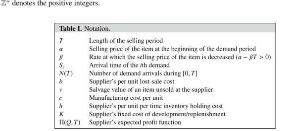
Figure 1 plots Π(10, T) for varying values of b for the instance stated in Example 2. As illustrated in Figure 1, typically, Π(Q, T) decreases after a certain value of T for fixed Q. Figure 1 also demonstrates that b has a larger impact on the behavior of Π(Q, T) at larger values of T. Four different values of b are considered. The optimum times to exit the market are 60.5, 29, 26.4, and 23.7 when b = 0, b = 10, b = 20, and b = 40, respectively. As the per unit lost-sale cost increases, it becomes more risky to stay in the market for long, in terms of the expected costs. Therefore, as b increases, the optimum market exit time decreases. Furthermore, the supplier’s expected profit is larger for smaller values of b, and the gap between the expected profits under two different b values becomes larger as T increases.
Proposition 4
Given a value of Q such that Q> 0, for very small values of T (i.e., as T → 0), we have Π(Q, T) ≈ −cQ − K + Qv − QhT + ( 𝛼 −𝛽T 2 + hT 2 − v ) 𝜆0T. (18)
Expression (18) can be interpreted as follows:𝜆0T is the mean number of demand arrivals within (0, T). The average
price for an item sold during this period is (
𝛼 −𝛽T2 ); therefore, the expected revenue is (
𝛼 −𝛽T2 )𝜆0T. The average savings
Figure 1.Supplier’s expected profits in Example 2 for varying b values.
from the holding cost of a sold item ishT
2. In other words, an item sold would incur an extra average holding cost of
hT
2 if it
remained unsold until the end of T time units. Therefore,𝜆0T ×hT
2 subtracted from QhT is the expected holding cost. The
average quantity that remains unsold at the end of T time units amounts to Q −𝜆0T, and they are salvaged at $v per unit.
The manufacturing cost and the replenishment cost for a starting inventory of Q units are cQ and K, respectively. When all these cost and revenue terms are considered, the supplier’s expected profits sum up to expression (18).
Recall from Section 1 that a price skimming strategy helps an inventor recover sunk costs rapidly. Let us assume that an inventing company aims for a minimum target profit of $𝜋 with the sales of Q units in a short amount of time T. Proposition 4 suggests that the supplier’s sunk costs should at most be equal to −cQ + Qv − QhT +
(
𝛼 −𝛽T2 +hT
2 − v
)
𝜆0T −𝜋 to achieve
target profit under the current pricing strategy and the market characteristics.
The next corollary that will be presented without a proof is a direct extension of Proposition 4 and follows from finding the domain of Q for which expression (18) is positive.
Corollary 1
For very small values of T, the supplier has positive expected profits for order quantities Q such that
Q< 𝜆0T ( 𝛼 −𝛽T2 +hT 2 − v ) − K c − v + hT . (19)
Under a price skimming strategy, Corollary 1 provides an upper bound on the replenishment quantity in order for the supplier to generate some positive profits after recovering sunk costs in a short amount of time. Corollary 1 also has an implication within the context of liquidation—that is, it quantifies the maximum level of inventory to be replenished for a soon-to-be-discontinued product.
Next, using a numerical example, we illustrate the behavior of Π(Q, T) with respect to T for a given Q considering varying values of v.
Example 3
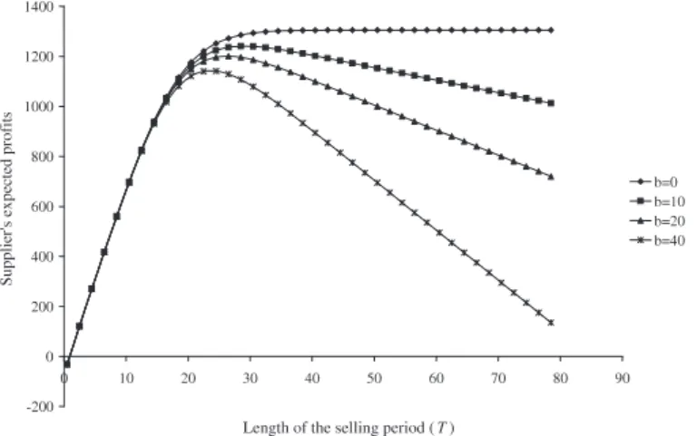
Consider a system with the following parameter values: c = 10, b = 6, h = 0.5, 𝜆0= 0.5, 𝛼 = 170, 𝛽 = 2, K = 20. Assume that Q is given as 40. Figure 2 shows a plot of Π(40, T) for v = 0, v = 2, v = 4, and v = 6.
As Figure 2 shows, Π(Q, T) is more sensitive to changes in v at small values of T. The reason is that when market exit time is small, there is a better chance that some of the items are going to be unsold. As T becomes larger, the salvage value
v has no effect on the expected profits, as indicated by the convergence of the four expected profit curves in Figure 2. This
implies that the salvage value of unsold items is an important parameter for an inventor aiming to exit the market after benefiting from high, short-term profits.
The following lemma further characterizes the behavior of the Π(Q, T) function with respect to T, for small enough values of T.
Lemma 1
For a given value of Q such that Q> 0, it follows that
Figure 2.Supplier’s expected profits in Example 3 for varying v values.
Figure 3.Illustration of the two cases of Lemma 1 on Example 4.
• if h⩽ 𝛽, Π(Q, T) is a concave function of T for small enough values of T, and • if h> 𝛽, Π(Q, T) is a convex function of T for small enough values of T.
Proof
The proof follows from taking the second-order partial derivative of expression (18) with respect to T.
Example 4
Consider a system with the following parameter values: c = 10, v = 5, b = 6, 𝜆0 = 0.5, 𝛼 = 170, 𝛽 = 2, K = 20. Assume that Q is given as 20. Figure 3 shows a plot of Π(20, T) for h = 4 and for h = 0.5.
Figure 3 illustrates the two cases of Lemma 1 on Example 4 by considering two different values of h. Given that𝛽 = 2, h = 0.5 refers to the case where h ≤ 𝛽, and hence, the supplier’s expected profit function is concave for small enough values of T. Similarly, h = 4 refers to the case where h > 𝛽 so that the supplier’s expected profit function is convex for small enough values of T.
Our analysis until this point concerned cases where either Q or T is given. Finding explicit expressions for the values of Q and T that jointly maximize the supplier’s expected profit function is quite challenging because of the complexity of expression (16). Therefore, we propose an algorithm that involves changing the value of T with increments of ΔT within a bounded range of T. A similar approach was proposed by Axsäter [35] for a different problem to maximize a complicated function with Poisson probabilities. Our algorithm utilizes Proposition 2 and the fact that 0⩽ T < 𝛼∕𝛽. Π∗refers to the
supplier’s expected profits at the optimum solution.
Algorithm I:
1. Set T = T∗= 0, Q∗= 0 and Π∗= 0.
2. Set T = T + ΔT. If T⩾ 𝛼∕𝛽, then stop. 3. Find the value of Q∗(T) using Proposition 2.
4. If Π(Q∗(T), T) > Π∗, then set T∗= T, Q∗= Q∗(T) and Π∗= Π(Q∗(T), T). Go to step 2.
It can be shown that the time complexity of the aforementioned algorithm is O ((Qu)(Tu∕ΔT)), where Qu and Tu are
upper bounds on Q and T. An upper bound on T is 𝛼∕𝛽, as suggested earlier. In the following section, we propose a parametric upper bound on Q that depends on T. In case of Poisson demand arrivals, this upper bound assumes a finite value for any T such that 0< T < 𝛼∕𝛽, and approaches to a linear increasing function of T as T becomes larger. Because
T is bounded, the worst-case complexity of the aforementioned algorithm is inverse proportional to ΔT.
5. An analysis of the general case
In this section, we report the results of our analytical and numerical analysis for the general case, that is,𝜆1 ≠ 0. In our analysis in Section 4 for the case of Poisson demand arrivals (i.e.,𝜆1 = 0), we showed that market exit time is an important decision variable that can increase the supplier’s expected profits when it is carefully decided. We also characterized the behavior of the supplier’s expected profits with respect to market exit time under varying problem parameters. Our objective in this section is to analyze how this behavior changes when demand arrivals are characterized by an NP process, particularly under different levels of demand sensitivity. Recall that when the increase in demand due to the decrease in price dominates the natural decrease in demand, we have 𝜆1 > 0. When the price decrease cannot help stimulate the demand enough, such that demand continues to decline over time, we have𝜆1 < 0. Therefore, for a particular setting, we model the higher sensitivity of the demand with respect to changes in price by larger values of𝜆1.
Because the price has to be positive, a natural upper bound on T is given by𝛼
𝛽, as in the special case of𝜆1 = 0. If𝜆1 < 0,
a second upper bound on T is implied by the fact that𝜆0+𝜆1T> 0. That is, we also have T < −𝜆0
𝜆1
. The next proposition involves the case of𝜆1 > 0 so that the only upper bound on T is 𝛼
𝛽. However, in order to gain some insights on how the
function Π(Q, T) behaves under very large values of T, in the next proposition, we momentarily relax this constraint on T.
Proposition 5
If𝜆1> 0, given a value of Q such that Q > 0, for very large values of T, we have
E[Lost-sale cost] ≈ b ( 𝜆0T + 𝜆1T2 2 ) − bQ.
Similar to the implication of Proposition 3, it is natural to expect that for𝜆1 > 0, there may exist a large enough value of T within
( 0,𝛼
𝛽
)
such that all the quantity is sold and the supplier only incurs lost-sale cost if he or she stays in the market thereafter. The lost-sales cost in this case increases in quadratic proportion to T. The next example illustrates how the supplier’s expected profits change with respect to T for varying values of per unit lost-sales cost b.
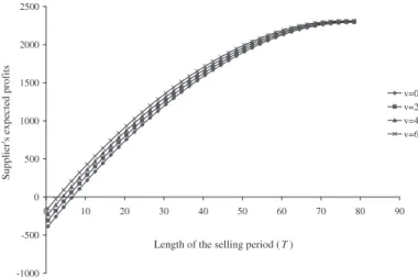
Example 5
Consider a system with the following parameter values: c = 10, v = 5, h = 0.5, 𝜆0 = 0.5, 𝜆1= 0.01, 𝛼 = 170, 𝛽 = 2, K = 20. Assume that Q is given as 10. Figure 4 shows a plot of Π(10, T) for four different values of b.
The difference in how the per unit lost-sales cost affects the supplier’s expected profits in the case of Poisson demand arrivals and NP demand arrivals when𝜆1 > 0 can also be observed by comparing Figure 4 with Figure 1. Specifically, the supplier’s expected profit in Figure 4 exhibits a concave decreasing behavior with respect to large T values, while it displays a linear decreasing behavior in Figure 1. The magnitude of the total expected lost-sales cost for a given T under different values of b can be quantified using Propositions 3 and 5.
The next proposition considers the case where market exit time attains very small values. An approximate analytical expression for the supplier’s expected profits is given for this case.
Proposition 6
Given a value of Q such that Q> 0, for very small values of T Π(Q, T) ≈ −cQ − K + Qv − QhT + ( 𝛼 − ( 3𝜆0+ 2𝜆1T)T ( 2𝜆0+𝜆1T)3 (𝛽 − h) − v ) ( 𝜆0T + 𝜆1T2 2 ) . (20)
562
Figure 4.Supplier’s expected profits in Example 5 for varying b values.
The interpretation of expression (20) is similar to that of expression (18). The expected number of items sold during (0, T) is ( 𝜆0T + 𝜆1T2 2 ) .
An item sold has an average value of
( 𝛼 − ( 3𝜆0+ 2𝜆1T)T ( 2𝜆0+𝜆1T)3 𝛽 ) ,
therefore, the expected revenue is ( 𝛼 − ( 3𝜆0+ 2𝜆1T)T ( 2𝜆0+𝜆1T)3 𝛽 ) ( 𝜆0T + 𝜆1T2 2 ) .
The average savings from the holding cost of a sold item is (( 3𝜆0+ 2𝜆1T)T ( 2𝜆0+𝜆1T)3 h ) . Therefore, QhT − (( 3𝜆0+ 2𝜆1T)T ( 2𝜆0+𝜆1T)3 h ) ( 𝜆0T + 𝜆1T2 2 )
is the expected holding cost that accumulates within (0, T). The expected number of items that are unsold is
Q − ( 𝜆0T + 𝜆1T2 2 ) ,
and they are salvaged at a rate of $v. When all these cost and revenue terms are considered along with the manufacturing cost and the replenishment cost, the supplier’s expected profits sum up to expression (20).
Assuming that an inventing company aims for a minimum target profit of $𝜋 with the sales of Q units in a short amount of time T, a similar interpretation to the one for Proposition 4 applies to Proposition 6. That is, Proposition 6 implies that the sunk costs of an inventing company should at most be equal to
− cQ + Qv − QhT + ( 𝛼 − ( 3𝜆0+ 2𝜆1T)T ( 2𝜆0+𝜆1T)3 (𝛽 − h) − v ) ( 𝜆0T + 𝜆1T2 2 ) −𝜋 (21)
563
Figure 5.Supplier’s expected profits in Example 6 for varying𝜆1values.
to achieve target profit under the current pricing strategy and market characteristics.
As an analog to Corollary 1, the next corollary follows from Proposition 6 and applies to the case of NP arrivals.
Corollary 2
For very small values of T, the supplier has positive expected profits for order quantities Q such that
Q< ( 𝜆0T + 𝜆1T2 2 ) ( 𝛼 −(3𝜆0+2𝜆1T)T (2𝜆0+𝜆1T)3 (𝛽 − h) − v ) − K c − v + hT . (22)
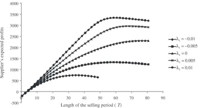
Next, we present an example to illustrate how the supplier’s expected profits and the optimum market exit time change under varying levels of demand sensitivity with respect to price changes. Recall that higher values of𝜆1for the same price function are an indicator of higher demand sensitivity in this setting.
Example 6
Consider a system with the following parameter values: c = 10, v = 5, h = 0.5, 𝜆0= 0.5, 𝛼 = 170, 𝛽 = 2, K = 20. Assume that Q is given as 40.
Figure 5 illustrates Π(40, T) in Example 6 for five different values of 𝜆1starting from −0.01 in increments of 0.005. As seen in Figure 5, the supplier’s expected profits for the same value of T increase with larger𝜆1. The optimum exit times from the market are 34.9, 59.1, 77.3, 68, and 59.6 for𝜆1 values of −0.01, −0.005, 0, 0.005, and 0.01, respectively. The optimum exit time from the market initially exhibits an increasing pattern with respect to larger𝜆1 values; however, after a period, it starts to decrease. The largest value of optimum market exit time is 77.4 for𝜆1 = −0.001. The reason for this behavior is that longer time in the market may initially be an opportunity for the supplier to increase expected profits by selling more due to higher demand associated with large𝜆1 values. However, this opportunity diminishes after a certain value of𝜆1and increasing demand rate leads to larger lost-sale cost thereafter. Therefore, for very large𝜆1values, it may be better to exit the market soon, whereas for small𝜆1values, staying in the market for a while may be an opportunity to increase expected profits.
In the next example, we illustrate the impact of discount per unit time, that is,𝛽, on the supplier’s expected profits for varying levels of T.
Example 7
Consider a system with the following parameter values: c = 10, v = 5, b = 6, h = 0.5, 𝜆0 = 0.5, 𝛼 = 170, K = 20. Assume that Q is given as 40.
Figure 6 illustrates Π(40, T) in Example 7 for three different values of the discount per unit time (i.e., for 𝛽 = 0.8, 𝛽 = 0.9, and𝛽 = 1) over 70.5 ⩽ T ⩽ 150.5. The example assumes that the corresponding rates of change in the demand intensity (i.e.,𝜆1) are −0.002, −0.001, and 0 for 𝛽 = 0.8, 𝛽 = 0.9, and 𝛽 = 1, respectively. The figure shows that, at smaller values of T (i.e., 70.5 ⩽ T ⩽ 99.5), the supplier’s expected profits are higher at a larger value of 𝛽 (i.e., 𝛽 = 1). For 100 ⩽ T ⩽ 127, 𝛽 = 0.9 leads to the largest expected profits, and for T ⩾ 127.5, 𝛽 = 0.8 results in the largest expected profits. This implies that the policy of decreasing prices to attract more demand is particularly effective when the length of the selling period is short. Taking both T and𝛽 as decision variables, we find that the supplier’s expected profits are
Figure 6.Supplier’s expected profits in Example 7 for varying𝛽 values.
maximized when𝛽 = 0.9 and T = 110.5. Furthermore, doing the same analysis by setting h to 0.1, we obtain 𝛽 = 0.8 and T = 132.5 as the optimum values of the decision variables. This implies that if holding costs are lower, the supplier is better off by staying in the market longer and gradually lowering the price.
Our results in Proposition 5, Proposition 6, and Corollary 2 are based on extreme values of T. In the next proposition, we propose an upper bound on the optimal value of Q given any T. Later, we will use this upper bound in developing an algorithm to optimize the supplier’s expected profit function over Q and T jointly.
Proposition 7
Given a value of T, an upper bound on the optimal value of Q is
Qu= (𝛼 − v + hT)E[N(T)]
c − v + hT . (23)
Algorithm II:
1. Set T = T∗= 0, Q∗= 0 and Π∗= 0.
2. Set T = T + ΔT. If T⩾ 𝛼∕𝛽, then stop.
3. For Q = 0 to Q =⌊Qu⌋, if Π(Q, T) > Π∗, then set T∗= T, Q∗= Q and Π∗= Π(Q, T). 4. Go to step 2.
Similar to that of Algorithm I, the time complexity of the aforementioned algorithm is O ((Qu)(Tu∕ΔT)), where Quand
Tu are upper bounds on Q and T. In case of NP arrivals, as E[N(T)] =(𝜆
0T +
𝜆1T2 2
)
, Quassumes a finite value for any
T such that 0 < T < 𝛼∕𝛽, and approaches to a polynomial increasing function of T as T becomes larger. Because T is
bounded, the worst-case complexity of the aforementioned algorithm is inverse proportional to ΔT.
6. Conclusions
In this paper, we have presented a model to analyze the ordering and market exit time decisions of an inventing company that applies skimming as a pricing strategy. The product under consideration is a new and trendy one with a short life cycle and high inventory holding costs. The market for the product is divided into different segments depending on the customers’ willingness to pay, and the prices are sequentially reduced for each customer segment [2, 4]. Considering that there may also be a gradual decrease in customer interest in the product over time, we have modeled the demand pattern using an NP process with a time-dependent rate. This approach has allowed us to take into account different types of demand intensity (increasing, decreasing, or stable) while answering questions Q1–Q9 raised in Section 1 as we summarize later.
Price skimming helps companies with innovative products recover their sunk costs in a short time and before the compe-tition steps in. Initially, the early adopters who are less sensitive to high prices are targeted. Our results have demonstrated that if the supplier plans to stay in the market for a limited duration, then the quantity to be replenished in order to gener-ate a profit is bounded (see Corollaries 1 and 2 as they relgener-ate to Q1). This bound highly depends on sunk costs besides the
other inventory-related parameters of the problem. Furthermore, we have provided an explicit upper bound on the value of sunk costs if the company is aiming to generate a target profit value in a short time (see Propositions 4 and 6 as well as expression (21) as they relate to Q1).
Our findings have revealed that the supplier’s expected profit is very sensitive to how long the product is sold in the market, and significant savings can be achieved if market exit time is carefully decided. With this premise, our analysis has indicated that for a given level of initial inventory, there exists an optimal value of market exit time after which the supplier’s expected profit is nonincreasing. In fact, we have shown that in the case of positive lost-sale cost, the supplier’s expected profit is a unimodal function of time to exit the market (see Examples 2 and 5 as they relate to Q2). Our characterization of the supplier’s expected profit function with respect to the market exit time is based on analytical and numerical results for the general case as well as the special case of Poisson demand arrivals.
We have also analyzed how the supplier’s expected profit and the optimum market exit time change for varying levels of demand sensitivity with respect to price (see Example 5 and Figure 4 as they relate to Q3). We have shown that increased demand sensitivity may be an advantage for amplifying the expected profit under the optimal market exit time. Furthermore, there exists a threshold value of demand sensitivity such that optimal market exit time increases up to the threshold value and decreases afterward. This, in turn, implies that decreasing prices may be a good practice for companies to achieve more profits in a short time if the demand is very sensitive to price. If the demand is not very sensitive to price, then extending the market exit time offers the maximum advantage of price skimming. As a result of investigating Q4, we propose procedures (Algorithms I and II) with worst-case time complexities for the supplier to make joint optimization decisions for market exit time and replenishment quantity.
Our analysis may be useful for managing an end-of-life product by offering insights about questions Q5–Q9. Specifically, Proposition 2 gives the optimal order quantity in the last replenishment of an end-of-life-cycle product for which market exit time is known. Propositions 3 and 5 can be used to quantify the impact of delayed market exit times (or product rollovers) on expected profits. Corollary 1 can be employed to find the maximum level of inventory to be replenished for a soon-to-be-discontinued product to generate some positive profits. Moreover, Example 7 and Figure 6 illustrate that the policy of decreasing prices to attract more demand is particularly effective when the length of the selling period is short.
Appendix A
A.1. Proof of Proposition 1
In order to calculate E[ ̄Uk], we use the density function of the kth order statistics of U1, U2, … , Un. Recalling Result (R1), this density function is given by
f̄U k(t) = n! (k − 1)!(n − k)!FU(t) k−1f U(t)(1 − FU(t))(n−k). (A.1)
FU(t) and fU(t) denote the distribution and density functions of Uidefined in Result (R3). Using expressions (9) and (10), we have FU(t) = m(t) m(T) = ∫t 0 ( 𝜆0+𝜆1s ) ds ∫T 0 ( 𝜆0+𝜆1s ) ds = t ( 𝜆0+𝜆1t∕2 ) T(𝜆0+𝜆1T∕2), (A.2) and fU(t) = 𝜆0+𝜆1t T(𝜆0+𝜆1T∕2). (A.3)
Substituting expressions (A.2) and (A.3) in expression (A.1) leads to
f̄U k(t) = n! (k − 1)!(n − k)! ( t(𝜆0+𝜆1t∕2) T(𝜆0+𝜆1T∕2) )k−1 𝜆 0+𝜆1t T(𝜆0+𝜆1T∕2) ( 1 − t(𝜆0+𝜆1t∕2) T(𝜆0+𝜆1T∕2) )n−k ,
and hence, E[ ̄Uk]is given by
n! (k − 1)!(n − k)!∫ T 0 ( 𝜆0+𝜆1t 𝜆0+𝜆1t∕2 ( t(𝜆0+𝜆1t∕2) T(𝜆0+𝜆1T∕2) )k( 1 − t(𝜆0+𝜆1t∕2) T(𝜆0+𝜆1T∕2) )n−k) dt. (A.4)
566
In order to simplify the aforementioned integral, we define x = t ( 𝜆0+𝜆1t∕2 ) T(𝜆0+𝜆1T∕2), (A.5) which leads to 𝜆1t2 2 +𝜆0t − T(𝜆0+𝜆1T∕2)x = 0. The two real roots of the aforementioned expression are given by
t1,2= −𝜆0∓ √ 𝜆2 0+ 2𝜆1T(𝜆0+𝜆1T∕2)x 𝜆1 .
Because we are interested in t> 0, we should have
t = −𝜆0+ √ 𝜆2 0+ 2𝜆1T(𝜆0+𝜆1T∕2)x 𝜆1 , and hence, 𝜆0+𝜆1t∕2 = 𝜆0+ √ 𝜆2 0+ 2𝜆1T(𝜆0+𝜆1T∕2)x 2 .
From expression (A.5), we have the following results: • If t = 0, then x = 0,
• If t = T, then x = 1,
• (𝜆0+𝜆1t)dt = T(𝜆0+𝜆1T∕2)dx.
Therefore, expression (A.4) simplifies to
E[ ̄Uk]= n (k − 1)!(n − k)!2(𝜆0+𝜆1T∕2)T ∫ 1 0 xk(1 − x)k 𝜆0+ √ 𝜆2 0+ 2𝜆1T(𝜆0+𝜆1T∕2)x dx. ■
A.2. Derivation of expression (12)
The derivation will follow by computing E[Revenue|N(T) = n] for 1 ⩽ n ⩽ Q and for Q < n < ∞ and utilizing these results in expression (6).
For 1⩽ n ⩽ Q, using Result (R3) and the independence of N(T) and Si, we can write
E [N(T) ∑ i=1 (𝛼 − 𝛽Si)|||| ||N(T) = n ] = E [ n ∑ i=1 ( 𝛼 − 𝛽 ̄Ui )] .
Observe that E[∑n1 ̄Ui]= E[∑n1Ui]because the sum of n random variables, whether they are ordered or unordered, is the same. This implies that for 1⩽ n ⩽ Q
E [ n ∑ i=1 ( 𝛼 − 𝛽 ̄Ui )] = 𝛼n − 𝛽E [ n ∑ i=1 Ui ] .
567
Using the density function of Uigiven in expression (A.3), it can be easily shown that E[Ui] = ( 3𝜆0+ 2𝜆1T)T ( 2𝜆0+𝜆1T)3 . Therefore, for 1⩽ n ⩽ Q E[Revenue|N(T) = n] = n ( 𝛼 − 𝛽 ( 3𝜆0+ 2𝜆1T)T ( 2𝜆0+𝜆1T)3 ) . (A.6)
For Q< n < ∞, we can write
E [ Q ∑ i=1 (𝛼 − 𝛽Si)|||| ||N(T) = n ] =𝛼Q − 𝛽E [ Q ∑ i=1 ̄Ui ] . (A.7)
Note that the value of E[ ̄Ui]in the aforementioned expression can be found using Proposition 1.
The rest of the derivation follows by utilizing expressions (A.6) and (A.7) in (6). ■
A.3. Derivation of expression (13)
The derivation will follow by computing E[Holding cost|N(T) = n] for 1 ⩽ n ⩽ Q and for Q < n < ∞ and utilizing these results in expression (7).
For 1⩽ n ⩽ Q, using Result (R3) and the independence of N(T) and Si, we have
E [N(T) ∑ i=1 Sih + (Q − N(T))hT|||| ||N(T) = n ] = E [ n ∑ i=1 ̄Uih + (Q − n)hT ] = nhE[Ui] + (Q − n)hT = nh ( 3𝜆0+ 2𝜆1T)T ( 2𝜆0+𝜆1T)3 + (Q − n)hT = QhT − nTh ( 𝜆1T + 3𝜆0 ) 3(2𝜆0+𝜆1T) . (A.8)
For Q< n < ∞, E[Holding cost|N(T) = n] should be computed using expression (11) and is given by
E[Holding cost|N(T) = n] = E [ Q ∑ i=1 Sih|||| ||N(T) = n ] = h Q ∑ i=1 E[ ̄Ui]. (A.9)
The result follows by utilizing expressions (A.8) and (A.9) in (7). ■
A.4. Proof of Proposition 2
We will first show that ̄Π(Q, T) is a strictly concave function of Q for all Q ∈ Z. Therefore, ̄Π(Q, T) − K is also a strictly concave function of Q in this range. This implies that its maximizer over Q ∈ {0} ∪Z+ is the smallest Q for which
̄Π(Q+1, T)− ̄Π(Q, T) < 0. As we will show later, the condition ̄Π(Q+1, T)− ̄Π(Q, T) < 0 leads to inequality (17). Finally,
we will compare the supplier’s expected profits resulting from an order of size ̄Q with those of an order of size 0. That is,
if ̄Π( ̄Q, T)− K > Π(0, T), we will conclude that Q∗(T) = ̄Q, else Q∗(T) = 0.
Let us start with proving the concavity of ̄Π(Q, T). Defining Δ ̄Π(Q, T) = ̄Π(Q + 1, T) − ̄Π(Q, T) and Δ2̄Π(Q, T) =
Δ ̄Π(Q + 1, T) − Δ ̄Π(Q, T), we will show that Δ2̄Π(Q, T) < 0. Using (16) and the fact that ̄Π(Q, T) = Π(Q, T) + K × 𝜅(Q), we have Δ ̄Π(Q, T) = −c(Q + 1) + (Q + 1)(v − hT)P{N(T) = 0} + Q+1 ∑ n=1 ( 𝛼n − 𝛽nT 2 + hnT 2 − (Q + 1)hT + (Q + 1 − n)v ) P{N(T) = n} + ∞ ∑ n=Q+2 ( 𝛼(Q + 1) −𝛽(Q + 1)(Q + 2)T 2(n + 1) − h(Q + 1)(Q + 2)T 2(n + 1) −(n − Q − 1) ) P{N(T) = n} + cQ − Q(v − hT)P{N(T) = 0} − Q ∑ n=1 ( 𝛼n −𝛽nT 2 + hnT 2 − QhT + (Q − n)v ) P{N(T) = n} − ∞ ∑ Q+1 ( 𝛼Q −𝛽Q(Q + 1)T 2(n + 1) − hQ(Q + 1)T 2(n + 1) − (n − Q)b ) P{N(T) = n}.
After some cancellation and rearrangement of terms, the aforementioned expression can be written as
Δ ̄Π(Q, T) = −c + (v − hT)P{N(T) = 0} + Q ∑ n=1 (−hT + v)P{N(T) = n} + ( 𝛼(Q + 1) − 𝛽(Q + 1)T 2 + h(Q + 1)T 2 − (Q + 1)hT ) P{N(T) = Q + 1} + ∞ ∑ n=Q+2 ( 𝛼 −𝛽(Q + 1)T (n + 1) − h(Q + 1)T (n + 1) + b ) P{N(T) = n} − ( 𝛼Q −𝛽Q(Q + 1)T 2(Q + 2) − hQ(Q + 1) 2(Q + 2) − b ) P{N(T) = Q + 1}.
Further rearrangement of the terms leads to
Δ ̄Π(Q, T) = −c + Q ∑ n=0 (v − hT)P{N(T) = n} + ( 𝛼 −𝛽(Q + 1) Q + 2 − h(Q + 1) Q + 2 + b ) P{N(T) = Q + 1} + ∞ ∑ n=Q+2 ( 𝛼 −𝛽(Q + 1)T n + 1 − h(Q + 1)T n + 1 + b ) P{N(T) = n}, and hence, Δ ̄Π(Q, T) = −c + Q ∑ n=0 (v − hT)P{N(T) = n} + ∞ ∑ Q+1 ( 𝛼 −𝛽(Q + 1)T n + 1 − h(Q + 1)T n + 1 + b ) P{N(T) = n}. (A.10)
569
Now, on the basis of the aforementioned expression, we are ready to compute Δ2̄Π(Q, T). Δ2̄Π(Q, T) = Q+1 ∑ n=0 (v − hT)P{N(T) = n} + ∞ ∑ Q+2 ( 𝛼 −𝛽(Q + 2)T n + 1 − h(Q + 2)T n + 1 + b ) P{N(T) = n} − Q ∑ n=0 (v − hT)P{N(T) = n} − ∞ ∑ n=Q+1 ( 𝛼 −𝛽(Q + 1)T n + 1 − h(Q + 1)T n + 1 + b ) P{N(T) = n},
which can be reduced to
Δ2̄Π(Q, T) = (v − hT)P{N(T) = Q + 1} + ∞ ∑ n=Q+2 ( − 𝛽T n + 1− hT n + 1 ) P{N(T) = n} − ( 𝛼 −𝛽(Q + 1)T Q + 2 − h(Q + 1)T Q + 2 + b ) P{N(T) = Q + 1}. It follows that Δ2̄Π(Q, T) = ( v − b −𝛼 +𝛽(Q + 1)T Q + 2 − hT Q + 2 ) P{N(T) = Q + 1} − ∞ ∑ n=Q+2 ( 𝛽T n + 1+ hT n + 1 ) P{N(T) = n}.
Because v< b, we have v − b < 0. A condition of 𝛼 and 𝛽 is that 𝛼 − 𝛽T ⩾ 0. Therefore, −𝛼 + 𝛽T ⩽ 0, which in turn implies that
−𝛼 +𝛽(Q + 1)T
Q + 2 ⩽ 0.
As a result, Δ2̄Π(Q, T) < 0, and hence, ̄Π(Q, T) is a strictly concave function of Q. Therefore, as discussed earlier, the
maximizer of ̄Π(Q, T) − K over Q ∈ {0} ∪ Z+, which is the same as the maximizer of ̄Π(Q, T) in this range, is the smallest
Q for which ̄Π(Q + 1, T) − ̄Π(Q, T) < 0. Now, we reduce expression (A.10) and provide different forms of it to write the solution as described by the condition ̄Π(Q + 1, T) − ̄Π(Q, T) < 0.
Observe that expression (A.10) can be rewritten as
Δ ̄Π(Q, T) = −c + (v − hT)P{N(T) ⩽ Q} + ∞ ∑ n=Q+1 ( 𝛼 −(𝛽 + h)T(Q + 1) n + 1 + b ) P{N(T) = n}. After substituting P{N(T) = n} = e −𝜆0T(𝜆 0T)n n!
in the aforementioned expression, we have
Δ ̄Π(Q, T) = −c + (v − hT)P{N(T) ⩽ Q} + (𝛼 + b)(1 − P{N(T) ⩽ Q}) −(𝛽 + h)(Q + 1)T 𝜆0T ∞ ∑ n=Q+1 e−𝜆0T(𝜆 0T) (n+1) (n + 1)! ,