Mutual Coupling Compensation in Transmitting Arrays of Thin Wire
Antennas
Sana Khan, Hassan Sajjad, Mehmet K. Ozdemir, and Ercument Arvas
Department of Electrical and Electronics Engineering Istanbul Medipol University, Kavacik, Beykoz 34810, Turkey
Abstract ─ This paper presents a numerical technique for the compensation of mutual coupling in transmitting arrays of thin wire antennas. The Method of Moments is used to compute the scattering parameters of the array. Using these parameters and the original excitations, a set of new excitation values are computed. The new excitation values compensate the effect of the mutual coupling. Computed results are given for linear, circular, and 3-Dimensional arrays. Uniform and binomial excitations are studied. Results obtained are compared with other available data and very good agreement is observed.
Index Terms ─ 3-Dimensional arrays, circular arrays, dipole antenna arrays, linear arrays, Method of Moments, mutual coupling compensation, planar arrays, transmitting arrays.
I. INTRODUCTION
In a simplistic array design approach the classical pattern multiplication method is used. In this method the radiation pattern of an array of identical antenna elements is the product of an element pattern and an array factor. The element pattern is the pattern of an isolated element with its center at the origin. This element is assumed to be excited by a unit voltage. The array factor is a sum of fields from isotropic point sources located at the center of each array element and is found from the elements excitation (amplitude and phase) and their locations [1]. Therefore, in the classical array theory, it is assumed that all the elements of the array have equal radiation pattern, in other words, the coupling between individual elements is ignored. For a practical array, this is not true since mutual coupling causes each element to see a different environment and consequently has a different radiation pattern from its neighboring elements. Mutual coupling between the antenna elements in an antenna array is a classical problem, which is responsible for the degradation of array performance [2–4]. The purpose of this work is to include the effect of mutual coupling and still produce the same pattern as the array
factor method.
(a) (b)
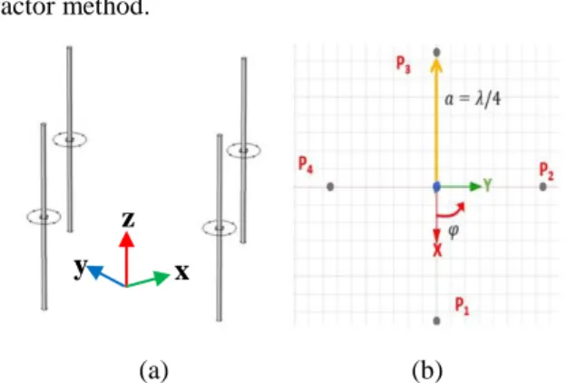
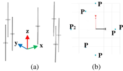
Fig. 1. (a) Circular array of four thin wire antennas with length λ/2. (b) Top view of the system.
However, this requires replacing the original excitations of the array with a new set of excitations. These new excitation values can be found if the scattering matrix of the array is measured or computed.
Here, the Method of Moments [5] is used to compute the scattering parameters of the array. For example, consider the circular array of four thin halfwave dipoles as shown in Fig. 1 (a). The radius of the circle is λ/4 and the radii of the dipoles are λ/200. Assume that the antennas are excited with the same magnitude and with phase progression of 30o. We call
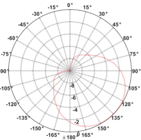
these excitations as the original excitations. The resulting pattern computed using these original excitations and classical array theory is shown in Fig. 2. We will call this result as the desired pattern. It is incorrect because the mutual coupling effects are not included in the classical approach. When mutual coupling effects are included, the pattern shown in Fig. 3 is obtained. We call this pattern the practical pattern and it is quite different than the desired pattern given in Fig. 2.
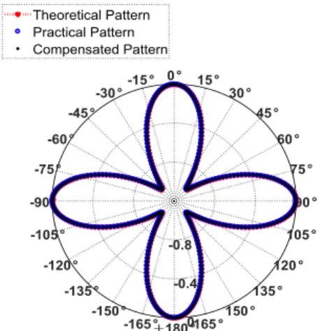
Using the method described in Section II, a set of new excitations for the array is computed. The true practical pattern of the array computed using these new excitations and by including mutual coupling effects is shown in Fig. 4. It is quite similar to the desired pattern
x
z
y
Submitted On: February 22,2018
of Fig. 2. In the next section, we will summarize a numerical method for computing the new excitations.
Several techniques to reduce mutual coupling and improve the isolation between antennas have been investigated [6–11]. Some of these include decoupling networks (DN) which use lumped elements and hybrid couplers to reduce mutual coupling. Another common technique uses the defected ground plane structure (DGS) in which the ground plane is modified by introducing slits of different shapes.
Inductance and capacitance are introduced using electromagnetic band gap (EBG) structures to create forbidden band of frequencies which helps in isolation of the antennas. Metamaterials are also used due to existence of band gaps in their frequency responses. Neutralization lines are also used to feed reverse current to lessen the amount of coupled current. All the techniques mentioned above increase complexity of the network in one way or another. Physical modification of the structure is required, e.g., introduction of lumped
elements, parasitic elements, and sometimes special materials may be required to reduce the mutual coupling.
This paper uses a non-invasive method in which the physical structure or design of the antenna is not changed. Only the excitation voltages of the antennas are changed and these new excitation voltages which are called compensated voltages produce a radiation pattern which is similar to the pattern obtained from pattern multiplication method with the original voltages. The pattern multiplication method uses the original excitations and assumes no mutual coupling between the elements. The resulting theoretical desired pattern is usually much different than the actual practical pattern as shown in the above example. On the other hand, the new pattern, obtained by using the compensated voltages and by assuming the existence of the mutual coupling does agree with the theoretical desired pattern. Only thin wire dipole antennas of lengths less than or equal to λ/2 are considered. Such antennas are usually called as single mode antennas. The individual elements in the array may or may not be identical in dimensions (length, wire radius). A number of similar methods have been suggested for the compensation of mutual coupling [12– 14]. This paper is an extension of the work published in [15]. Here, in addition to simple linear arrays we consider circular and 3-Dimensional arrays. We also consider linear arrays with non-uniform excitations.
II. COMPUTATION OF COMPENSATED
VOLTAGES
Consider a transmitting array of N identical elements. Each element is assumed to be driven by a voltage source,
Vgk, for k = 1,2,...,N. All sources are assumed to have an
Fig. 2. The desired pattern (theoretical pattern using array factor) of circular array of four halfwave dipole antennas excited with uniform phase progression.
Fig. 3. The practical pattern of circular array of four halfwave dipole antennas excited with uniform phase progression.
Fig. 4. Theoretical pattern obtained using the classical pattern multiplication method and the original sources (solid), the true practical pattern obtained using the original sources (dashed-dotted), and the compensated pattern obtained using the compensated voltages (dashed).
identical internal impedance of Zo. When mutual coupling
is ignored, the input impedance, Zin, of all antennas are the
same. Then, the current entering the kth element is simply,
𝐼𝑘 = 𝑉𝑔𝑘
𝑍𝑜+𝑍𝑖𝑛. (1)
The pattern of the kth element is basically fixed by this I k.
The array multiplication method assumes this pattern for the kth element. This is the ideal desired pattern.
In a practical array, because of the existence of mutual coupling, the actual input impedance of the kth
element, 𝑍𝑘′𝑖𝑛, is not anymore equal to Zin. Hence, the
actual current entering the kth element is now given by,
𝐼′𝑘= 𝑉𝑔𝑘 𝑍𝑜+𝑍
𝑘𝑖𝑛′
. (2) Since this current is different than Ik, the pattern of this
antenna will be different. However, if instead of Vgk we
use a new voltage, 𝑉′𝑔𝑘=
𝑉𝑔𝑘(𝑍𝑜+𝑍𝑘𝑖𝑛′ )
𝑍𝑜+𝑍𝑖𝑛 , (3)
then, the current entering the kth element will be equal to
Ik and hence the pattern of the kth element will be the same
as the desired pattern. It is not easy to measure 𝑍𝑘′𝑖𝑛
directly. However, the scattering matrix of the array can be computed or measured easily. As shown in Appendix, the new compensated voltages can be obtained in terms of the original voltages and the S-matrix as follows,
[𝑉𝑔′] = 2𝑍0
𝑍𝑜+𝑍𝑖𝑛{𝑈 − 𝑆}
−1[𝑉
𝑔]. (4)
Where U represents an N × N unit matrix, S is the N × N matrix of the scattering parameters of the array, [Vg]
and are [𝑉𝑔′] column vectors showing the original and
compensated voltages, respectively.
In this work the scattering matrix of the array is computed using the Method of Moments. The feeds are modeled by magnetic frill currents. The unknown currents are approximated by piece-wise sinusoidal functions and Galerkin’s method is used for matching [16]. Using the moment matrix and its inverse, one can compute the open circuit parameter matrix, short circuit parameter matrix and hence the scattering parameter matrix of the array. The details are available in [17–19].
III. NUMERICAL RESULTS
Results are given for three different arrays: (i) Circular array of four wire antennas, (ii) Linear array of five wire antennas, and (iii) 3-Dimensional array of seven wire antennas. For each case three different patterns are computed. The theoretical pattern is computed using pattern multiplication method which uses the original voltages and assumes no mutual coupling. The practical pattern is computed using the original voltages but including the effect of mutual coupling. Finally, the compensated pattern is computed using the newly computed voltages and assuming the presence of mutual coupling. Note that all patterns computed in this work are normalized. The results are
verified using COMSOL Multiphysics® [20]. A. Circular array of four antennas
In this section, four halfwave dipole antennas have been arranged in a circular array of radius a = λ/4. The elements are identical with radius λ/200. The number of expansion functions used for all the MoM simulations are 63 per antenna. In order to find the array factor for the circular array of four dipole antennas, the antennas are replaced by four isotropic sources at their centers, as shown in Fig. 1 (b). The radiation pattern of such an array can be found easily using pattern multiplication method. The element pattern of a halfwave dipole antenna in the H-plane is a unit circle. Since the total pattern is the product of the element pattern and array factor, then the total pattern, in this case, is equal to the array factor. The array factor is given by,
𝐴𝐹 = ∑4
𝑛=1𝑉𝑛𝑒𝑗𝛽(𝑥𝑛sin𝜃cos𝜑+𝑦𝑛sin𝜃sin𝜑), (5)
where β is the wave number and Vn is the complex input
voltage at nth antenna.
A.1. Uniform excitation of circular array
In the first case we excite the array uniformly with
V = 1 V. The compensated voltages were computed to be
equal to 𝑉′= 1.75∠45𝑜 for each antenna element.
Figure 5 shows, the three computed patterns in the H-plane. At first sight, it might be surprising to see that the theoretical and the practical patterns are identical, as if there was no mutual coupling between the elements. Of course there is mutual coupling as indicated by the compensated voltage being different than the original one, however, due to the symmetry of the structure and uniform excitations the effect of mutual coupling is automatically compensated. This can be seen by examining the current distributions on the antennas as shown in Fig. 6. Note that although the magnitude of the currents is different, their distribution and hence their radiation patterns are identical.
Fig. 5. Radiation pattern (H-plane) for four element circular array of halfwave dipole antennas with uniform excitation.
A.2. Non-uniform excitation
In this case the elements (P1, P2, P3, and P4) in Fig.
1 (b) are assumed to be excited with voltages V1 =1∠0𝑜,
V2 =1∠30𝑜, V3 =1∠60𝑜, and V4 =16∠90𝑜, respectively.
The computed compensated voltage values are 𝑉1′=
3.06∠78𝑜, 𝑉
2′= 2.29∠82𝑜, 𝑉3′= 1.32∠134𝑜, and 𝑉4′=
0.29∠ − 92𝑜. The three computed patterns are shown
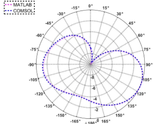
in Fig. 4. The current distribution on the antennas are shown in Fig. 7. It can be seen that the currents are not symmetric which explains the significant difference in the patterns of Fig. 4. Figure 8 compares our computed practical patterns with those of COMSOL and excellent agreement is observed. Figure 9 compares three patterns computed by (i) using (5), (ii) using MoM with compensated voltages, and (iii) using COMSOL with compensated voltages.
IV. LINEAR ARRAY OF FIVE
ANTENNAS
Here we consider a linear array of five identical halfwave dipoles as shown in Fig. 10 with inter-element spacing of 0.1λ. A binomial excitation of the linear array with V1 = 0.25∠180𝑜, V2 = 1∠90𝑜, V3 = 1.5∠0𝑜, V4 = 1∠
90𝑜, and V
5 = 0.25∠180𝑜 was used. Figure 11 compares
the theoretical and the practical patterns for this array.
It is seen that because of mutual coupling the practical pattern is much different than theoretical pattern although both methods use the same original excitations. The computed compensated voltage values are 𝑉1′=
2.05∠84𝑜, 𝑉
2′= 2.47∠126𝑜, 𝑉3′= 3.86∠135𝑜, 𝑉4′=
2.47∠126𝑜, and 𝑉
5′= 2.05∠84𝑜. Figure 12 compares
the compensated pattern, computed using these new voltage values, with the theoretical pattern computed using array factor method with original voltages. It is observed that the use of the new voltages has
x
z
y
Fig. 10. Linear array of five halfwave dipole antennas uniformly spaced with a separation of 0.1λ.
250
0 50 100 150 200
No. of Expansion Functions
0 1 2 3 4 5 6 7 8 9 10 Theoretical Currents Practical Currents Compensated Currents
Fig. 6. Current distribution for uniformly excited four halfwave dipole antennas arranged in a circular array.
250 200 150 100 50 0
No. of Expansion Functions
0 2 4 6 8 10 12 14 Theoretical Currents Practical Currents Compensated Currents
Fig. 7. Current distribution of circular array of four halfwave dipole antennas with a progressive phase excitation.
Fig. 9. Comparison of compensated pattern for four element circular array of halfwave dipole antennas (H-plane).
Fig. 8. Comparison of practical pattern for circular array in H-plane.
compensated the effect of mutual coupling to a considerable extent.
V. COMPENSATION OF 3-DIMENSIONAL
ARRAYS
In this section, a 3-Dimensional array is studied. As shown in Fig. 13 (a), seven dipoles are arranged in two circles.
Four dipoles are placed along a circle in the lower ring and three dipoles in the upper circular ring which is displaced along z-axis. The dipoles are identical, having length L=λ/2 and radius a=λ/200. The centers of the dipoles in the lower ring are at z=0 plane whereas the centers of the upper dipoles are at z=λ/4 plane. When the elements of the array shown in Fig. 13 (b) are excited by V1 = 1∠0o, V2 = 0.5∠180o, V3 = 1.5∠0o, V4 = 0.75∠180o,
V5 = 1∠0o, V6 = 0.5∠0o, and V7 = 0.75∠0o, then the
computed compensated voltages are given by 𝑉1′=
4.9∠89. 6𝑜, 𝑉
2′= 5.8∠ − 94𝑜, 𝑉3′= 6.3∠87. 8𝑜, 𝑉4′=
5.12∠ − 130𝑜, 𝑉
5′= 3.7∠82. 5𝑜, 𝑉6′= 4.56∠ − 128. 6𝑜,
and 𝑉7′= 2.48∠100. 4𝑜. The patterns in the three
principle planes can be seen in Figs. 14, 15, and 16. It is seen that the newly computed voltages compensate the effect of mutual coupling to a large extent.
(a) (b)
Fig. 15. YZ-plane pattern for 3-dimensional array. Fig. 11. Comparison of theoretical pattern and practical
pattern for the five element linear dipole array using binomial excitation (H-plane).
Fig. 12. Comparison of theoretical pattern and compensated pattern for the five element linear dipole array (Fig. 10) using binomial excitation (H-plane).
P 1 P2 P 3 P 4 P 5 P 7 x z y P 6
Fig. 13. (a) Three-dimensional dipole array with seven elements. Four dipoles are placed along a circle of radius 0.5λ and three dipoles along a radius of 0.4λ which are moved in the z-direction by λ/4. (b) Top view of the system.
VI. CONCLUSION
In this work the effect of mutual coupling in transmitting arrays of thin wire antennas has been effectively compensated. This is established without changing the antenna structure but only modifying the excitation voltages. These modified excitation voltages were computed using the scattering matrix of the array which was computed using a simple moment method technique. Three different arrays and different methods of excitations were considered. In some cases, the effect of mutual coupling was drastic compared to others. The effect of mutual coupling was successfully reduced in all cases. The patterns computed were verified with COMSOL. The limitation of this method is that it only applies to transmitting arrays. The extension of this simple method to receiving antenna array is not straight forward. In the transmitting case the excited ports are actual physical ports, whereas in the receiving case the excitation source is far away shown by the (N+1)th port
which brings some complications. We are in the process of developing a simple method for the receiving antenna array.
ACKNOWLEDGMENT
This work was partially supported by TUBITAK (TURKEY) under the project number 215E316.
A. APPENDIX
Using transmission line theory, we know that the current entering the kth antenna can be expressed as,
𝐼𝑘 = 𝑉𝑘+−𝑉𝑘−
𝑍0 , (A.1)
where 𝑉𝑘+is the forward (incident) voltage entering the kth
antenna of the N-port network defined by, 𝑉𝑘+=
𝑉𝑔𝑘′
2 , (A.2)
and 𝑉𝑘− is the reflected voltage from the kth antenna It can
be written as,
𝑉𝑘− = 𝑆𝑘1𝑉1++ 𝑆𝑘2𝑉2++ ⋯ 𝑆𝑘𝑁𝑉𝑁+,
= (𝑆𝑘1𝑉𝑔1′ + 𝑆𝑘2𝑉𝑔2′ + ⋯ 𝑆𝑘𝑁𝑉𝑔𝑁′ )/2.
(A.3) Where, Sij is the element of the scattering matrix for the
system. Substituting the values of (2) and (3) in (1) we get, 𝐼1 = (𝑉1+− 𝑉1−)/𝑍0, = 𝑉𝑔1 ′ (2𝑍0) − (1/𝑍0){𝑆11𝑉1++ 𝑆12𝑉2+… 𝑆1𝑁𝑉𝑁+}, = 1 (2𝑍0) {𝑉𝑔1′ − 𝑆11𝑉𝑔1′ − 𝑆12𝑉𝑔2′ … 𝑆1𝑁𝑉𝑔𝑁′ }, (A. 4) 𝐼2= 1 (2𝑍0){𝑉𝑔2 ′ − 𝑆 21𝑉𝑔1′ − 𝑆22𝑉𝑔2′ … 𝑆2𝑁𝑉𝑔𝑁′ }, (A.5) 𝐼𝑁= 1 (2𝑍0){𝑉𝑔𝑁 ′ − 𝑆 𝑁1𝑉𝑔1′ − 𝑆𝑁2𝑉𝑔2′ … 𝑆𝑁𝑁𝑉𝑔𝑁′ }. (A.6)
The above equations can be written in matrix form as, [ 𝐼1 𝐼2 ⋮ 𝐼𝑁 ] = 1 2𝑍0 [ 𝑉𝑔1′ 𝑉𝑔2′ ⋮ 𝑉𝑔𝑁′ ] − 1 2𝑍0 [ 𝑆11 𝑆12 … 𝑆1𝑁 𝑆21 𝑆22 … 𝑆2𝑁 ⋮ ⋮ ⋮ ⋮ 𝑆𝑁1 𝑆𝑁2 … 𝑆𝑁𝑁 ] [ 𝑉𝑔1′ 𝑉𝑔2′ ⋮ 𝑉𝑔𝑁′ ] ,
or in short hand notation as, [𝐼] = 1
2𝑍0{𝑈 − 𝑆}[𝑉𝑔
′]. (A.7)
Here, [I] is the N×1 column vector of the desired input currents. U is N×N unit matrix and [𝑉𝑔′] is the N×1
column vector of the desired compensated source voltages feeding the antennas. Then, the desired compensated source voltages (in the presence of mutual coupling) are given by, [𝑉𝑔′] = (2𝑍0){𝑈 − 𝑆}−1[𝐼], (A.8) or [𝑉𝑔′] = (2𝑍0){𝑈 − 𝑆}−1 [ 𝑉𝑔1 𝑍0+𝑍1 𝑉𝑔2 𝑍0+𝑍2 ⋮ 𝑉𝑔𝑁 𝑍0+𝑍𝑁] .
Where, 𝑍𝑖, is the input impedance of the 𝑖𝑡ℎ element.
When the elements are identical (A.8) reduces to (4).
REFERENCES
[1] W. L. Stutzman and G. A. Thiele, Antenna Theory
and Design. 3rd Ed., John Wiley & Sons Inc., 2013.
[2] H. T. Hui, M. E. Bialkowski, and H. S. Lui, “Mutual coupling in antenna arrays,” International
Journal of Antennas and Propagation, vol. 2010,
pp. 1-7, 2010.
[3] C. Craeye and D. Gonzlez-Ovejero, “A review on array mutual coupling analysis,” Radio Science, vol. 46, no. 2, 2011.
[4] M. K. Ozdemir, E. Arvas, and H. Arslan, “Dynamics of spatial correlation and implications on MIMO systems,” IEEE Communications Magazine, vol. 42. no. 6, pp. S14-S19, June 2004.
[5] R. F. Harrington, Field Computation by Moment Fig. 16. XZ-plane pattern for 3-dimensional array.
Methods. Wiley-IEEE Press, 1993.
[6] A. C. J. Malathi and D. Thiripurasundari, “Review on isolation techniques in MIMO antenna systems,”
Indian Journal of Science and Technology, vol. 9,
no. 35, 2015.
[7] H. T. Hui, “Decoupling methods for the mutual coupling effect in antenna arrays: A review,”
Recent Patents on Engineering, vol. 1, no. 2, pp.
187-193, Jan. 2007.
[8] C. H. Niow, Y. T. Yu, and H. T. Hui, “Compensate for the coupled radiation patterns of compact transmitting antenna arrays,” IET Microwaves,
Antennas Propagation, vol. 5, no. 6, pp. 699-704,
Apr. 2011.
[9] M. Zamlynski and P. Slobodzian, “Comment on ‘compensate for the coupled radiation patterns of compact transmitting antenna arrays’,” IET
Microwaves, Antennas Propagation, vol. 8, no. 10,
pp. 719-723, July 2014.
[10] A. G Demeryd, “Compensation of mutual coupling effects in array antennas,” IEEE Antennas and
Propagation Society International Symposium. 1996 Digest, vol. 2, pp. 1122-1125, July 1996.
[11] H. Sajjad, S. Khan, and E. Arvas, “Mutual coupling reduction in array elements using EBG structures,”
2017 International Applied Computational Electro-magnetics Society Symposium Italy (ACES), pp.
1-2, Mar. 2017.
[12] S. Henault and Y. M. M. Antar, “Comparison of various mutual coupling compensation methods in receiving antenna arrays,” IEEE Antennas and
Propagation Society International Symposium, pp.
1-4, June 2009.
[13] H. S. Lui, H. T. Hui, and M. S. Leong, “A note on the mutual-coupling problems in transmitting and receiving antenna arrays,” IEEE Antennas Propag.
Mag., vol. 51, no. 5, pp. 171-176, 2009.
[14] H. Steyskal and J. S. Herd, “Mutual coupling compensation in small array antennas,” IEEE
Trans. Antennas Propag., vol. 38, no. 12, pp.
1971-1975, 1990.
[15] S. Khan and E. Arvas, “Compensation for the mutual coupling in transmitting antenna arrays,”
2016 IEEE Asia-Pacific Conference on Applied Electromagnetics (APACE), pp. 84-88, Dec. 2016.
[16] W. L. Stutzman and G. A. Thiele, Antenna Theory
and Design. 1st Ed., John Wiley & Sons Inc., 1981.
[17] G. V. Eleftheriades and J. R. Mosig, “On the network characterization of planar passive circuits using the method of moments,” IEEE Transactions
on Microwave Theory and Techniques, vol. 44, no.
3, pp. 438-445, Mar. 1996.
[18] B. Hamdi, T. Aguili, N. Raveu, and H. Baudrand, “Calculation of the mutual coupling parameters and their effects in 1-D planar almost periodic
structures,” Progress in Electromagnetics Research, vol. 59, pp. 269-289, 2014.
[19] S. Khan, “Compensation of Mutual Coupling in Transmitting Arrays of Thin Wire Antennas,”
Master’s Thesis, Istanbul Medipol University,
Turkey, 2017.
[20] COMSOL Multiphysics, V5.2a, Stockholm, Sweden, 2016.
Sana Khan received her B.S. degree in Engineering Sciences from Ghulam Ishaq Khan Institute (GIKI) of Engineering Sciences and Tech-nology, Topi, KPK, Pakistan in 2013 and M.S. degree from Istanbul Medipol University, Istanbul, Turkey in August 2017. Currently, she is pursuing her Ph.D. degree in Electrical Engineering at the same university. Her research interests include computational electromagnetics, antennas, and optical communication.
Hassan Sajjad received his B.S. degree in Telecommunication Engin-eering from FAST-NUCES Peshawar, Pakistan in 2009 and M.S. degree in Electrical Engineering from Linnaeus University, Vaxjo, Sweden in 2012. Since 2015, he is pursuing his Ph.D. degree in Electrical Eng-ineering at Istanbul Medipol University, Istanbul, Turkey. His research interests include numerical electro-magnetics, RF/Microwave devices, and antennas.
Kemal Ozdemir received the B.S. and M.S. degrees in Electrical Eng-ineering from Middle East Tech-nical University, Ankara, Turkey in 1996 and 1998, respectively, and the Ph.D. degree in Electrical Engin-eering from Syracuse University, Syracuse, NY in 2005. Currently, he is with the Electrical and Electronics Engineering Department of Istanbul Medipol University, Istanbul, Turkey. His research interests include channel modelling, PHY layer design, parameter estimation, and 5G massive MIMO systems.
Ercument Arvas was born in 1953, in Van, Turkey. He received his B.Sc. and M.Sc. degrees in electrical engineering from the Middle East Technical University, Ankara, Turkey, in 1976 and 1979, respectively, and his Ph.D. degree in electrical engineering from Syracuse University, Syracuse, NY, USA, in 1983. From 1983 to 1984, he was with the Department of Electrical Engineering, Yildiz Technical University, Istanbul, Turkey. Between 1984 and 1987, he was with Rochester Institute of Technology, Rochester, NY, USA, and from 1987 to 2014, he was with Syracuse University. He is now teaching at the Electrical and Electronics Engineering Department, Istanbul Medipol University, Istanbul, Turkey. His research interests include electromagnetics scattering and microwave devices. Dr. Arvas is a Fellow of the Electromagnetics Academy.