Deep learning based unsupervised tissue segmentation in histopathological images

DEEP LEARNING BASED UNSUPERVISED

TISSUE SEGMENTATION IN

HISTOPATHOLOGICAL IMAGES

a thesis submitted to

the graduate school of engineering and science

of bilkent university

in partial fulfillment of the requirements for

the degree of

master of science

in

computer engineering

By

Troya C

¸ a˘

gıl K¨

oyl¨

u

November 2017

DEEP LEARNING BASED UNSUPERVISED TISSUE SEGMEN-TATION IN HISTOPATHOLOGICAL IMAGES

By Troya C¸ a˘gıl K¨oyl¨u November 2017

We certify that we have read this thesis and that in our opinion it is fully adequate, in scope and in quality, as a thesis for the degree of Master of Science.

C¸ i˘gdem G¨und¨uz Demir(Advisor)

Hamdi Dibeklio˘glu

Pınar Karag¨oz

Approved for the Graduate School of Engineering and Science:

Ezhan Kara¸san

ABSTRACT

DEEP LEARNING BASED UNSUPERVISED TISSUE

SEGMENTATION IN HISTOPATHOLOGICAL IMAGES

Troya C¸ a˘gıl K¨oyl¨u M.S. in Computer Engineering Advisor: C¸ i˘gdem G¨und¨uz Demir

November 2017

In the current practice of medicine, histopathological examination of tissues is essential for cancer diagnosis. However, this task is both subject to observer variability and time consuming for pathologists. Thus, it is important to de-velop automated objective tools, the first step of which usually comprises image segmentation. According to this need, in this thesis, we propose a novel ap-proach for the segmentation of histopathological tissue images. Our proposed method, called deepSeg, is a two-tier method. The first tier transfers the knowl-edge from AlexNet, which is a convolutional neural network (CNN) trained for the non-medical domain of ImageNet, to the medical domain of histopatholog-ical tissue image characterization. The second tier uses this characterization in a seed-controlled region growing algorithm, for the unsupervised segmentation of heterogeneous tissue images into their homogeneous regions. To test the ef-fectiveness of the segmentation, we conduct experiments on microscopic colon tissue images. Quantitative results reveal that the proposed method improves the performance of the previous methods that work on the same dataset. This study both illustrates one of the first successful demonstrations of using deep learning for tissue image segmentation, and shows the power of using deep learn-ing features instead of handcrafted ones in the domain of histopathological image analysis.

Keywords: Deep learning, convolutional neural networks, transfer learning, histopathological tissue image segmentation, seed-controlled region growing.

¨

OZET

H˙ISTOPATOLOJ˙IK G ¨

OR ¨

UNT ¨

ULERDE DER˙IN

¨

O ˘

GRENME TEMELL˙I ¨

O ˘

GRET˙IC˙IS˙IZ DOKU

B ¨

OL ¨

UTLEMES˙I

Troya C¸ a˘gıl K¨oyl¨u

Bilgisayar M¨uhendisli˘gi, Y¨uksek Lisans Tez Danı¸smanı: C¸ i˘gdem G¨und¨uz Demir

Kasım 2017

G¨un¨um¨uz tıbbında, dokuların histopatolojik incelenmesi, kanserin te¸shisinde ¨

onemli rol oynamaktadır. Fakat bu i¸slem, hem g¨ozlemci de˘gi¸skenli˘gine a¸cık, hem de patologlar i¸cin zaman alıcıdır. Dolayısıyla, otomatik nesnel ara¸cların geli¸stirilmesi ¨onemlidir. Bu ara¸cların ilk basamakları genellikle g¨or¨unt¨un¨un b¨ol¨utlenmesidir. Bu ihtiyaca y¨onelik olarak, bu tez ¸calı¸smasında, histopatolo-jik doku g¨or¨unt¨ulerinin b¨ol¨utlenmesi i¸cin, deepSeg adını verdi˘gimiz iki a¸samalı metodla, yeni bir yakla¸sım sunuyoruz. ˙Ilk a¸sama, AlexNet adlı ve medikal ol-mayan ImageNet alanında e˘gitilmi¸s evri¸simli yapay sinir a˘gında saklanan bil-giyi, medikal alanda bulunan histopatolojik doku g¨or¨unt¨us¨u karakterizasyonu i¸cin aktarmaktadır. ˙Ikinci a¸sama ise bu karakterizasyonu, ¸cekirdek kontr¨oll¨u bir b¨olge b¨uy¨utme algoritmasında kullanarak, heterojen doku g¨or¨unt¨ulerini homo-jen b¨olgelerine ¨o˘greticisiz olarak b¨ol¨utlemektedir. Bu b¨ol¨utlemenin do˘grulu˘gunu test etmek i¸cin, mikroskobik kolon dokusu g¨or¨unt¨ulerinde testler yapılmı¸stır. Elde etti˘gimiz sayısal sonu¸clar, ¨onerdi˘gimiz metodun, aynı veri k¨umesi ¨uzerinde ¸calı¸san di˘ger metodların performanslarını arttırdı˘gını g¨ostermi¸stir. Bu ¸calı¸sma, hem derin ¨o˘grenme tekniklerini doku g¨or¨unt¨u b¨ol¨utlemesi i¸cin kullanan ilk ba¸sarılı ¨

orneklerden biri olarak yerini almı¸s; hem de histopatolojik g¨or¨unt¨u analizinde de-rin ¨o˘grenme temelli ¨ozniteliklerin, elle ¸cıkarılanlara ¨ust¨un geldi˘gini g¨ostermi¸stir.

Anahtar s¨ozc¨ukler : Derin ¨o˘grenme, evri¸simli yapay sinir a˘gları, aktarmalı ¨

o˘grenme, histopatolojik doku g¨or¨unt¨u b¨ol¨utlemesi, ¸cekirdek kontroll¨u b¨olge b¨uy¨utmesi.

Acknowledgement

I primarily want to thank my advisor C¸ i˘gdem G¨und¨uz Demir. Not only she determined the direction of this thesis study, she also provided key guidance and continuous help that made it possible for me to finalize this study. I cannot envisage how this study would be possible without her. Likewise, I would also like to thank my thesis committee members Hamdi Dibeklio˘glu and Pınar Karag¨oz. Their valuable comments helped the improvement of this study and lead it to its final state. I also cannot forget my colleagues in the Computer Engineering department. Starting from my lab piers Can Fahrettin Koyuncu and Simge Y¨ucel, I want to thank all my friends in the department for their invaluable support and friendship.

By completing this thesis study, I come to an end of a phase in my educational life. It has been around seven years since I started studying in Bilkent Univer-sity. My undergraduate study in Electrical and Electronics Engineering and my masters study in Computer Engineering helped me to gain numerous attributes; both academic and social. I therefore want to thank all the students, staff and faculty such as Ebru Ate¸s, Ayhan Altınta¸s, Erman Ayday, Varol Akman, Daniel DeWispelare, Engin Soyupak, ˙Ilgi Ger¸cek; and all the friends that I met here. I feel very privileged to have been here for a such long time.

Of course, I would like to thank the people who helped me to obtain this privilege, namely my previous teachers such as ˙Irfan and S¸ebnem Cant¨urk, my acquaintances from TED Ankara College high-school, my family and especially my mother Meltem Keskin. Without her support and determination for my education throughout my life, I would not be able to achieve any of this. So it is possible to say that she is the real architect behind anything I achieve.

With the eventuality of this thesis study, I feel the joy of making a dribblet of contribution to the scientific literature. This was all possible due to visionaries such as ˙Ihsan Do˘gramacı and Mustafa Kemal Atat¨urk, who valued knowledge and science over all.

Contents

1 Introduction 1

1.1 Motivation . . . 2

1.2 Contribution . . . 3

2 Background 6

2.1 Deep Convolutional Neural Networks . . . 6

2.2 Transfer Learning . . . 11

2.3 Related Work . . . 12

3 Methodology 16

3.1 Tier 1: Transfer Learning from AlexNet to Supervised Homoge-neous Tissue Image Classification . . . 17

3.1.1 CNN Model Training . . . 18

3.2 Tier 2: Unsupervised Heterogeneous Tissue Image Segmentation from Supervised Homogeneous Tissue Image Classification . . . . 24

CONTENTS vii 3.2.2 Region Growing . . . 29 3.2.3 Post-processing . . . 31 4 Experiments 33 4.1 Dataset . . . 33 4.2 Evaluation . . . 35 4.3 Comparisons . . . 37 4.4 Parameter Selection . . . 39 4.4.1 Parameters of Tier 1 . . . 39 4.4.2 Parameters of Tier 2 . . . 41 4.5 Results . . . 42 4.6 Discussion . . . 49 5 Conclusion 56

List of Figures

1.1 Sample tissue image for illustrating adenocarcinoma . . . 5

2.1 A sample CNN model . . . 8

3.1 The end product of Tier 1 . . . 17

3.2 The AlexNet model . . . 20

3.3 Resulting filters of the first convolutional layer . . . 21

3.4 Resulting filters of the second convolutional layer . . . 22

3.5 Resulting filters of the third convolutional layer . . . 22

3.6 Resulting filters of the fourth convolutional layer . . . 23

3.7 Resulting filters of the fifth convolutional layer . . . 23

3.8 Schematic overview of Tier 2 . . . 25

3.9 A sample image from SegmentationSet . . . . 26

3.10 Illustration of initialization and seed identification steps, on a sam-ple image . . . 29

LIST OF FIGURES ix

3.11 Illustration of the region growing step on a sample image . . . 31

3.12 Illustration of the post-processing step on a sample image . . . 32

4.1 An example image for each category in AuxiliarySet . . . . 34

4.2 A sample image from SegmentationSet. . . . 35

4.3 Gold standard version of the image shown in Figure 4.2 . . . 36

4.4 Visual effects of the area threshold . . . 45

4.5 Visual results of the deepSeg method . . . . 48

List of Tables

3.1 Essential layers of the used AlexNet model . . . 19

4.1 Quantitative results on the training set . . . 43

4.2 Comparative quantitative results for the test set . . . 46

4.3 Quantitative results obtained on the test set . . . 50

4.4 Quantitative results on the test set by using Variation 1 . . . 52

Chapter 1

Introduction

In the diagnosis and treatment selection of cancer, accurate interpretation of pathological results plays an important role [1, 2]. With the development of technology, the variety in its treatment has increased; different diagnosis results in a different treatment selection. However there may exist disagreements on the diagnosis among pathologists. Depending on the case, the overall process may be significantly complex and subjective. Additionally, there is a significant increase in the number of cases. Digital pathology on the other hand provides faster and more objective decisions, and thus, they start to play an important role as a diagnostic tool [3].

The typical first step of such a tool is segmentation, which aims to separate regions of different properties in a histopathological image. In this study, for facilitating the diagnosis of colon adenocarcinoma, a cancer type which accounts for 90-95% of all colorectal cancers, we present a deep-learning based two-tier unsupervised segmentation method, which we call deepSeg. In its first tier, we use highly effective deep convolutional neural networks (CNN) to learn the char-acterization of tissue formations. In this tier, we use the available information previously learned from a vast collection of natural images by using a technique called transfer learning. In the second tier, we use the obtained characteriza-tions to divide a histopathological image into its normal and cancerous regions.

This tier uses a seed-controlled region growing algorithm. Our overall end prod-uct method therefore is able to delineate the homogeneous regions in an unseen histopathological colon tissue image. To illustrate the effectiveness of our method, we conduct experiments on annotated images and compare the evaluation results with the previously developed methods. These results show that deepSeg, the method which we propose in this thesis, outperforms previous methods and it is a viable method to be considered in the future of computational pathology.

The overview of this chapter and others as follows; first, the motivations that drove us to devise our segmentation method and our resulting contributions to the literature are mentioned in this chapter. Next, in Chapter 2, background in-formation necessary to follow the discussion in other chapters are presented, with the existing studies in the literature. In presenting the background information, a discussion about artificial neural networks is not included; this topic is assumed to be readily available. Rather, convolutional neural networks are presented as they emerged much more recently. In Chapter 3, our two-tier methodology is presented. Lastly in Chapter 4, the experimental performance of our method is shown in comparison with the other methods, with also including information about the experimental dataset. Analysis and discussion about the results, work done and potential future work concludes the thesis.

1.1

Motivation

In commencing this study, we have two main motivations as driving forces. These are:

• Insufficient usage and exploration of deep learning systems in the domain of digital pathology and especially for its segmentation problem, although they were proven to be effective in many computer vision tasks.

• The need for a top performance system in the domain of pathology that constantly becomes more and more complicated.

The first motivation is explored in more detail when the previous related work is introduced in Section 2.3. However, as a foreword, it can be stated that the use of deep learning and convolutional neural networks in the domain of digital pathology is rare, where especially convolutional neural networks are shown to work effectively in various image related tasks [4]. The second motivation follows the first one, where we believe that using these networks for the purpose of segmentation will both improve upon the results of previous studies, and thus, will form a basis for further improvements. This kind of an improvement is necessary to overcome additional issues created by the never ending development of technology and complication in the domain. Likewise, we also feel that any novel learning system that becomes the state-of-art in image processing must be employed in digital pathology for the hopes of gaining better results, in this case; convolutional neural networks.

1.2

Contribution

Following from our motivations, the main contributions of this study are twofold. First, our proposed deepSeg method uses deep learning features to character-ize histopathological images. Majority of the studies dedicated to image seg-mentation in this domain use hand-crafted features, which makes them highly task-specific. Furthermore, in obtaining deep learning based features, we trans-fer knowledge from a non-medical domain, which is again one of the first such applications. With this study, we showcase the effectiveness of using convolu-tional neural networks in image related tasks, and their ability to learn image characterizations that enables more accurate image processing.

Our second contribution is related to the way we process histopathological images once we obtained deep-learning based characterizations. Our use of this characterization in segmentation is different than the standard approach em-ployed by the previous studies. After dividing the image into its pixels or equal-sized patches that contain a collection of pixels, these studies usually define class labels for their pixels/patches and use these labels for segmentation. In other

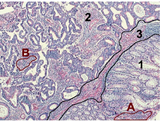
words, in these studies, there is one-to-one correspondence between class labels and region types. They assign each pixel/patch to one of the classes and form connected components with the ones that belong to the same class label. The seg-mentation that they obtain is a result of this straightforward operation. However, this approach can be problematic, because there can be some small regions that are visually different than their regions of interest, meaning that they do not and should not affect the overall region type. Such examples can be seen in Figure 1.1, namely the regions labelled with A and B (see the figure for detailed explanation). Simply defining a class label per region type and using class labels for segmenta-tion in these cases raises addisegmenta-tional issues as training a classifier becomes harder, and the trained classifier may mislabel these pixels/patches that correspond to those subregions. Thus in our proposed method, our classifier learns more classes (including normal and various cancer types) than the types of the regions to be segmented. This extended characterization is used in a region growing algorithm, which is able to use more information to determine patch-region similarity that the region will grow upon, rather than just connecting patches/pixels with the same label.

Figure 1.1: Sample tissue image for illustrating adenocarcinoma. This work focuses on unsupervised segmentation of colon images that contain normal and adenocarcinomatous regions. Colon adenocarcinoma accounts for 90-95% of all colorectal cancers, thus being the most common form of cancer in colon tissues. This cancer type originates from glandular epithelial cells and causes deformations in glands. Nonglandular stromal regions that are found in between glands, are irrelevant in the context of colon adenocarcinoma diagnosis. On the figure, such a subregion (marked with 3) can be included in either a normal (marked with 1) or a cancerous (marked with 2) region, without changing the region’s type. Furthermore, such nonglandular subregions (marked with A and B) are found in both normal and cancerous regions.

Chapter 2

Background

The study in this thesis is constructed on a two-tier operation; unsupervised seg-mentation of histopathological tissue images based on supervised learning of a deep convolutional neural network. The aim of this chapter is to include any necessary background information that will be referred in discussing our method-ology. The structure is as follows; first, deep convolutional neural networks are reviewed (Section 2.1). Then, for the use of the special training method, trans-fer learning in the context of deep convolutional neural networks is examined (Section 2.2). Lastly, related work on the subject is mentioned (Section 2.3).

2.1

Deep Convolutional Neural Networks

Starting with the McCulloch-Pitts artificial neuron model, there have been nu-merous attempts to capture biological computation, which is the essence of human intelligence [5]. Now, neural networks play an important role in the field of ma-chine learning by solving numerous tasks. An emerging issue however; there is no-free-lunch in learning (artificial) intelligence tasks. This means that, there is no single algorithm or model that captures the nature or essence of all possible situations [6, 7]. For standard artificial neural networks (these networks are also

called as fully connected neural networks, due to the fact that all inputs of their layers are connected to all neural/computational elements) this problem emerges for data of large sizes, like images. To capture the nature of large data, a straight-forward application is to increase the depth and width of the network. But when this is done, obtained performance is most generally very poor, where training data evaluation performance is high but test data (the data that was not used during training) evaluation performance is poor. This is a phenomenon called overfitting, and it is related to memorization rather than learning.

To alleviate this problem for image related tasks, a specialized artificial neural network model was devised. Taking its inspirations from biological sensory neu-rons [8], the deep convolutional neural network (DCNN or CNN for short) was proposed. This model can be thought as a (generally) deeper neural network. Like regular neural networks, CNNs must be trained with training data using (typically) backpropagation learning algorithm. After the training phase, the forward-pass operation of this network can be used to evaluate unseen data. The problems arising with increasing depth are solved by using specialized layers for hidden layers, before the regular fully connected ones. One of the most important properties of some of these layers is that they greatly reduce the number of pa-rameters that must be learned. This reduction is an important solution to many learning based issues if done efficiently. Just like a regular neural network, a CNN is a trainable black-box estimation and the important types of layers employed are explained here. Note that each of these layers can be thought as volume trans-formers, where they transform an input volume into an output. Some layers alter the input volume size, while others do not. An example is shown in Figure 2.1.

The sample CNN shown in Figure 2.1 is composed of three convolutional layers and two pooling layers, whose details will be explained shortly. One aspect visible from the image is the transformation of the volume. For instance, the input volume of size 28 × 28 is transformed into a volume of size 24 × 24 × 4 by the convolutional layer. And the pooling layer transforms this volume into a volume of size 12 × 12 × 4. At the end, the aforementioned data size reduction can be observed– namely, a proceeding fully connected layer must process 26 elements rather than 28 × 28. In this understanding, now, the detailed information on

Figure 2.1: A sample CNN model from [9]. This image is used under the permis-sion of the copyright owner: The MIT Press.

individual layers are presented.

• Convolutional layer: This layer is the most essential layer of a CNN. The inspiration for this layer is from the brain anatomy, as it is thought that some layers of sensory neurons perform filtering on their input. Therefore this layer performs filtering, in other words, convolution on its input and learned filter. Apart from the biological connotation, this layer is very efficient in keeping the number of variables to be learned in acceptable levels. A non-specialized fully connected layer has to independently learn all its weight variables, the number of which is H × W × Z × L; where H, W , and Z are input dimensions and L is the number of neurons in the layer. This is necessary as all neurons are connected to all inputs, and there is a weight parameter for each of them. A convolutional layer on the other hand, uses shared weights as filters. The filter is the same for all input patches, and it can be thought as if it slides through the input area. As the training operation proceeds, calculated updates for the same filter positions are aggregated and applied as the same to result in again same weights. Therefore, the number of independent variables to be learned are reduced to Hk× Wk× N ; where Hk, and Wk are filter dimensions and N is

the number of filters. As expected, the latter is much smaller– in our study for instance, images that are inputted to the first (convolutional) layer of our network are of size 227 × 227 × 3 (so naturally L should also be large in

a fully connected layer), but the filters that we use are of dimensions than 11 × 11 × 3 and there are 96 of them.

The output of this layer can be regarded as a volume of filtering outputs for different filters, merged on the third dimension. The obtained volume after this layer’s operation will be of size [(H − Hk+ 2P )/S + 1] × [(W − Wk+

2P )/S + 1], where P is pad– the parameter used to determine the amount of pixels that are added to the borders of the input (with techniques such as mirroring and zero-padding) and S is stride– the parameter that determines the number of pixels that the sliding window slides after each iteration of the convolution. A common practice is to select filter dimensions equal (Hk and Wk). Another common practice is to select P and S such that

the obtained output is the same size with the input, in height and width. One last point in this layer is; a filter’s depth matches the depth of the input. For instance, if the input of the layer is an RGB image, the filters of this layer are of depth three. At each sliding iteration, a three dimensional convolution is applied, where each corresponding input and filter entry are multiplied and their results are added to make a single number.

• Nonlinearity layer: This layer is inspired from the nonlinear input-output behavior of the biological neuron. This layer maps the input to a limited real range nonlinearly. A direct benefit is thus the limitation of the numeric range. Most common used types of nonlinear functions in this layer are Sigmoid and Rectified Linear Unit (ReLU ). Sigmoid function is defined as S(x) = _1+e1−x. ReLU is defined as f (x) = max(0, x). As the only operation

accomplished by this layer is the mapping of input to an output depending on the funciton in use, there is no learning needed.

• Pooling layer: This layer can be viewed as a compressor of information. Again for this layer, stride and kernel size parameters must be selected, just like the convolutional layer. With these selections, a sliding window which has the size determined by the kernel is traversed through the input volume. At each iteration, one number is produced over an area. Then the stride parameter is used to determine the slide of the window. According to these parameters, the input volume is converted to a much smaller output volume.

The common usage is to select these parameters to create a non-overlapping slide, such that the output surface area is four or sixteen times smaller than the input area. An important point here is that the sliding windows in this layer are two-dimensional, where convolutional layer windows are typically three-dimensional (whose third dimension can be of any size). Therefore, the output volume of this layer has the same depth with its input’s volume.

There are two common modes of operation for this layer; maximum and av-erage pooling. Maximum pooling compresses the information by taking the maximum value at each sliding window iteration, whereas average pooling takes the average of the values inside the window. Again note that there is no learning required in this layer.

• Fully connected layer: This layer is the basic neural network layer. For every neuron in this layer, a weight is assigned and learned for each input element. The operation of this layer can be viewed as an inner product between the input vector and the learned weight matrix.

In a typical CNN, one or more convolutional, nonlinearity and pooling layers are paired in this order, before one or more fully connected-nonlinearity layer pair. In a classification system, the last layer is a fully connected (decision) layer, with the number of outputs (or neurons) selected as the number of input classes. Here, each output signifies the class probability of the input (when the softmax function is used on the results of the decision layer). The class with the maximum probability is therefore selected as the class of the input. Another key difference between CNNs and regular neural networks is that in CNNs, the fully connected layer is inputted with a much smaller input size and thus, a much smaller number of fully connected layer parameters like neurons and weights are needed. Overall, this results in a limited number of independent variables that must be learned or adjusted in the training phase– a feature that helps to overcome overfitting.

2.2

Transfer Learning

One can employ different strategies when training a CNN on a dataset. Here, a number of them are presented. Note that these methods are not exhaustive; using other techniques, or using a mixture of these techniques are also viable.

1) Learning from scratch: When the dataset is adequately large, a training

operation that starts on randomized weights can eventually avoid over-fitting [10].

2) No additional training: A pre-trained CNN model can be used without

any further training. Outputs of one of its layers can be treated as features, and they can be used to train other classifiers or evaluators, such as support vector machines (SVMs).

3) Fine-tuning: A pre-trained network can also be used in other ways than

a feature extractor. One can take a pre-trained network, modify it or not, and start (or continue) training iterations on another dataset.

Transfer learning in deep learning is the transfer of knowledge between source and target models [11, 12]. In that context, note that the options two and three described here can be used to relay information between models. In this work, the fine-tuning option is employed (thus we use the words training and fine-tuning interchangeably to refer the learning process of our CNN). When a pre-trained model is selected for fine-tuning, there is no need to use the same dataset, or the exact model. A generally employed scheme is to take a model that was trained on an extensive image dataset, and resume training on a new but limited image dataset. Due to the weight sharing property of convolutional layers, there is no need to scale the new dataset images to the same size, or preserve all layers. Only data size preservation problem arises in the last fully connected layers. Therefore, a plausible strategy is to change and train incompatible last layer(s) from scratch, while training exported layers with a smaller weight update rate. This strategy is plausible because of the inner workings of a CNN– a pre-trained

CNN on natural images shows a phenomenon where early layers learn general and low level features such as Gabor filters and later layers learn task specific high level features [13]. Such kind of transfer learning has been successfully applied for many computer vision tasks; including image recognition [11], segmentation [14], and video classification [15].

2.3

Related Work

Existing studies on tissue segmentation generally rely on using handcrafted fea-tures. These studies typically partition an image into primitives (patches, pixels or objects) and they characterize these primitives using the handcrafted features. These primitives are then merged based on their extracted features to form seg-mentations.

Patch-based studies divide the histopathological images into equal sized patches. From these patches, they extract handcrafted color and texture features from the pixels inside these patches, and classify them based on these features. Then, they form the segmentation by connecting the patches of the same class. In this understanding, Mete et al. extract features from the results of color based clustering [16]. They train a support vector machine (SVM) on these features, and with the patches that this classifier identifies as positive, the delineation is obtained. Wang et al. extract statistical texture features from their slides [17]. Again by using a SVM, they obtain the segmentation as a result of a classifica-tion process consisting of multiple steps. Romo et al. split an image into a grid of blocks, where each block is represented by the feature spaces of color, inten-sity, orientation, and texture [18]. Target and distractor examples are picked for learning, and similarity metrics allow to find clusters of these examples in the feature spaces. A probability map is obtained by integrating similarity maps of each subspace, which allows for the selection of regions of interest.

Pixel-based studies’ follow a similar approach. However, they omit the step of patch divide, and directly classify pixels using their handcrafted features. Then,

they merge the pixels of the same class to form segmented regions. Mosaliganti et al. use a three-step process where in the first step, they label each pixel belonging to one of the four microstructural components based on color [19]. Following this, they obtain correlations, which are eventually used as features for the final classification, that forms the segmentation. Signolle et al. uses wavelet-transform to subsample very large histopathological images. On these samples, they construct hidden Markov tree models for the classification of pixels [20]. This study also includes the merging of classifiers, which are obtained for different hidden Markov trees for different hyper-parameter selections.

Lastly, object-based studies represent an image with a set of objects that corre-sponds to approximate locations of histological tissue components. They charac-terize each object with the spatial distribution of other objects within the specified neighborhood. In these studies, the handcrafted features are obtained for object-level textures, which are used by a region growing algorithm to merge the objects for forming the segmentation. Tosun et al. obtain their objects by locating cir-cular primitives on pixel collections that are grouped by color intensities [21]. The segmentation that follows is obtained based on defined measures of these objects, by using a region growing algorithm. In another study, again Tosun et al. introduce a texture measure to quantify the spatial relations of tissue compo-nents [22]. For that, this study defines a run-length matrix on constructed graph nodes, similar to defining a run length matrix on gray pixel values, and extracts texture features from this graph run-length matrix. S¸im¸sek et al. define their ob-jects similarly and quantify their distribution by defining the cooccurence matrix on this object set [23]. Then they use a multilevel graph partitioning algorithm that uses this quantification to achieve segmentation.

Only a few studies use deep learning based features to segment histopatholog-ical tissue images. In the study by Xu et al., the overall aim is to segment an image into two regions of interest; epithelial and stromal [24]. It accomplishes this task using three handcrafted feature based methods versus variations of CNN feature based methods. The CNN method uses patch based processing (patches can be obtained by simply sliding a window or using other algorithms), paired with classifiers of softmax and support vector machines. In this study, patches are

directly assigned to their classification labels to obtain the final segmentation. In the end, this study shows that CNN based approaches outperform handcrafted feature based approaches. Also, Arevalo et al. use CNNs to detect basal cell carcinoma regions [25]. For this task, the presented method is a four step algo-rithm. In the first step, it uses autoencoders or independent component analysis to obtain a set of feature detectors for the input image. In the second step, the image is characterized with using the obtained feature detectors by using the CNN approach. Here, an interesting point is that this method does not use stan-dard training for the CNN model it uses. The CNN model here is merely used for its forward pass operation, where there is only one convolutional layer and one pooling layer, and its convolutional layer uses the feature detectors obtained in the previous step as filters. Based on the extracted features, in the third step, it trains a binary classifier, that indicates whether cancer is present in an im-age or not. Finally in the last step, it uses visualization techniques to illustrate which regions in the image are related with cancerous patterns, which can also substitute for a segmentation.

Rather than these studies, there also exist other studies that focus on tation using deep learning. However, these ones do not focus on tissue segmen-tation, which aims to segment a heterogeneous tissue image into its biologically meaningful homogeneous regions. Instead, they focus on (segmenting) nuclei in medical images, which aims to differentiate nuclear objects from the background. First, Xing et al. use a CNN based method to segment nucleus regions from the rest of the medical image [26]. In this study, a CNN that is trained on patch size images is used to generate a probability map on pixels, which corresponds to how likely a pixel belongs to a part of a nucleus. Then, an iterative region merging algorithm is used on this map to mark the nuclei. Sirinukunwattana et al. have the aim of detecting nuclei, using a CNN [27]. The CNN is used to assign probabilities to each pixel being the center of a nuclei, in a sliding window manner to process patches. They then finalize the detection using local maxima in the probability map.

Finally, there is only one work to our knowledge that combines deep learn-ing, transfer learning and medical image related tasks. Shin et al. use a cou-ple of known CNN models that have been previously used, for detection and classification tasks in the medical domain [28]. Both transfer learning (includ-ing fine-tun(includ-ing and feature usage without additional train(includ-ing) and train(includ-ing from scratch are used as training strategies on these models. The findings reveal that transfer learning from natural image datasets can be beneficial in medical image processing tasks.

Chapter 3

Methodology

Our proposed method relies on using deep learning for unsupervised tissue seg-mentation. This method, which we call deepSeg, is based on a two-tier operation. In Tier 1, a convolutional neural network (CNN) is used to learn the character-ization of histopathological images. We transfer a CNN that is pre-trained on a natural image dataset with the technique defined in Section 2.2. When trained with homogeneous tissue images in a supervised manner (the details of the used images, namely, differences between homogeneous and heterogeneous images, will be explained shortly), this model characterizes its input image with six posteri-ors, corresponding to six classes. Tier 2 then uses learned characterizations to segment a heterogeneous image into its homogeneous regions in an unsupervised manner. To accomplish that, these heterogeneous images are divided into over-lapping patches. Using the CNN model from the first tier, each patch is char-acterized by six posteriors. This characterization is initially used to determine homogeneous seed regions. These seeds are then grown using our region growing algorithm to encompass the whole image. Lastly, our post-processing algorithm finalizes the segmentation.

Before delving into the details of both tiers, it is beneficial to briefly mention the properties of the images that are used in the first and second tiers. In Tier

1, the images used to train the CNN model belong to a dataset called Auxiliary-Set. This set contains patch size homogeneous images. The images are called as homogeneous, because one image contains normal or cancerous tissue of a single cancer type. In Tier 2, the images used for segmentation are from a dataset called SegmentationSet. These images are heterogeneous and they are much larger than the patch size. As heterogeneity implies, the same image may contain both nor-mal and cancerous regions. The details of these datasets will be provided in Section 4.1.

3.1

Tier 1:

Transfer Learning from AlexNet

to Supervised Homogeneous Tissue Image

Classification

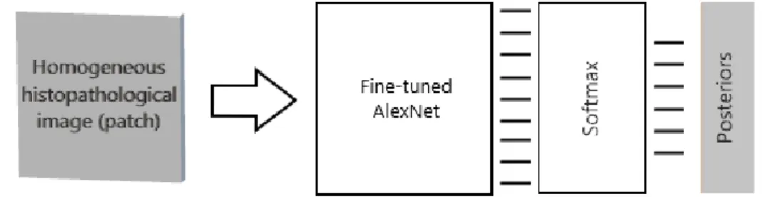
The aim of this tier is to obtain a CNN model that fairly characterizes homoge-neous histopathological images. For this purpose, this tier transfers the knowledge from a pre-trained CNN model to our domain in a supervised manner, by fine-tuning (or further training) this CNN. Figure 3.1 shows the desired operation obtained at the end of this tier. In the following subsection, we first elaborate on the training procedure of the CNN, and then provide a collection of visual results obtained at the end of this tier’s operation.

Figure 3.1: The end product of Tier 1. The desired CNN model after fine-tuning is expected to produce six posteriors that fairly characterize a homogeneous histopathological image. The decision layer indicated by “Softmax” is trained from scratch, to work as a classifier on top of the transferred information from previous layers of fine-tuned AlexNet. Details are specified in Section 3.1.1.

3.1.1

CNN Model Training

The CNN model that we use to train or fine-tune is AlexNet [29], that was originally trained for the ImageNet natural image dataset [4] for the challenge in 2010. The ImageNet dataset was constructed for an annual challenge where teams compete to train models to obtain highest evaluation accuracies in classifying unseen images. According to the numbers of 2010, there were approximately 15 million images and 1000 (high-level) classes. The AlexNet model achieved the best results in many classification categories over 1.2 million evaluation images. Their CNN consists of five convolutional layers, three max-pooling layers, and three fully connected layers to result in 60 million parameters and 650 000 neurons [29].

We use the Caffe [30] framework for CNN training. The AlexNet model they provide is a slight modification, that was trained on the ILSVRC12 challenge dataset for 310 000 iterations. The layers of the used model are given in Table 3.1, in their usage order. For completeness, the input, although not being a layer, is also included.

In Table 3.1, the first column specifies the type of layers. The second column supplies the values of the variables that characterize these layers. As can be seen, there are four different kinds of layers (excluding input information, which is self-explanatory). A convolutional layer is characterized by its filter kernel size, stride and pad it uses, and the number of outputs that it produces. A nonlinearity layer is only characterized by the nonlinear function it uses to produce its outputs. A pooling layer is characterized by its mode of operation, kernel filter size, and stride it uses. Lastly, a fully connected layer is characterized by the number of outputs it produces (more detailed information about CNN layers can be found in Section 2.1). Note that the decision layer in AlexNet produces 1000 posteriors, for the 1000 high-level ImageNet classes. Therefore, as the information learned in this layer is highly task specific; it must be omitted. This layer is learned from scratch– its weights are randomly initialized, and the number of outputs are set to six, which is the number of classes in our AuxiliarySet.

Table 3.1: Essential layers of the used AlexNet model [29]. Other (utility) layers of varying kinds are omitted in this representation.

Layer Name Layer Information

Input 227 × 227 × 3 (RGB) image

Convolutional number of outputs: 96, kernel size: 11, stride: 4, pad: 0 Nonlinearity type: ReLU

Pooling type: MAX, kernel size: 3, stride: 2

Convolutional number of outputs: 256, kernel size: 5, stride: 1, pad: 2 Nonlinearity type: ReLU

Pooling type: MAX, kernel size: 3, stride: 2

Convolutional number of outputs: 384, kernel size: 3, stride: 1, pad: 1 Nonlinearity type: ReLU

Convolutional number of outputs: 384, kernel size: 3, stride: 1, pad: 1 Nonlinearity type: ReLU

Convolutional number of outputs: 256, kernel size: 3, stride: 1, pad: 1 Nonlinearity type: ReLU

Pooling type: MAX, kernel size: 3, stride: 2 Fully Connected number of outputs: 4096

Nonlinearity type: ReLU

Fully Connected number of outputs: 4096 Nonlinearity type: ReLU

Fully Connected number of outputs: 1000

to be set. The first one is the base learning rate baseη, which is the initial rate of

weight update. The second one is the multiplier γ, which is multiplied with the current learning rate η to obtain the new learning rate when a certain number of iterations passes. That certain number of iterations is the stepsize S. The next one is numiter, the number of iterations required for the completion of training.

The last one is the momentum α, which affects the weight update rate. For each weight, if the previous update was large, the current update becomes also large on account of this parameter. Else, it becomes smaller. In our experiments, we use the following values for these parameters: baseη = 0.001, γ = 0.8, S = 2000,

numiter= 15000, α = 0.9.

The AlexNet model whose parameters are defined in Table 3.1 is illustrated in Figure 3.2. In this figure, the volume parameters are written next to appropriate positions. The first volume is the input, and max pooling operations are defined on the figure. The last three operations, where arrows are coded with the word

Figure 3.2: The AlexNet model defined in [29]. Used model parameters are given in Table 3.1. This image is used under the knowledge of NIPS Proceedings and permission of one of the copyright owner authors: Alex Krizhevsky.

“dense” belong to the fully connected layers. Other unmarked operations are convolutions. In this figure, the volumes are divided into two equal portions after the first convolutional layer. This division is intended to divide the operations related to top and bottom volumes into two graphics processing units.

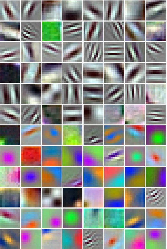
As explained, in Tier 1 of our method, we start with the pre-trained AlexNet model and fine-tune its weights using the images of AuxiliarySet. Fig-ures 3.3, 3.4, 3.5, 3.6, and 3.7 illustrate the learned weights (filters) of each of the five convolutional layers, respectively. Note that the first convolutional layer fil-ters are three dimensional, so they are illustrated as RGB images. An important observation here is a lot among the first layer filters developed into orientations of Gabor filters. These filters are widely applied in image recognition tasks, as they extract orientation dependent frequency contents, such as edges [31]. This development coincides with the understanding that earlier CNN layers extract low-level features like edges. Starting with the filters of the second convolutional layer, the filters lose their connotation as they become more and more high-level and task specific. One last note is that relative dimensions of the filters among different figures are not to scale.

Figure 3.3: Resulting filters of the first convolutional layer, after fine-tuning. As the filter depth in this layer is three, the filters are illustrated as RGB images.

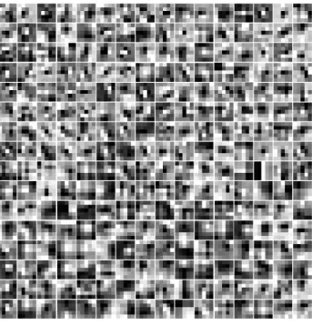
Figure 3.4: Resulting filters of the second convolutional layer, after fine-tuning. As the filter depth in this layer is larger than three, only the first dimension is illustrated.

Figure 3.5: Resulting filters of the third convolutional layer, after fine-tuning. As the filter depth in this layer is larger than three, only the first dimension is illustrated.

Figure 3.6: Resulting filters of the fourth convolutional layer, after fine-tuning. As the filter depth in this layer is larger than three, only the first dimension is illustrated.

Figure 3.7: Resulting filters of the fifth convolutional layer, after fine-tuning. As the filter depth in this layer is larger than three, only the first dimension is illustrated.

3.2

Tier 2: Unsupervised Heterogeneous Tissue

Image Segmentation from Supervised

Ho-mogeneous Tissue Image Classification

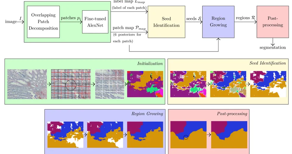
The aim of this tier is to segment a heterogeneous histopathological images into its homogeneous regions, in an unsupervised manner. The overall operation is sum-marized in Figure 3.8. This tier accomplishes this by a four-step seed-controlled region growing algorithm. First, the heterogeneous image is divided/decomposed into overlapping patches. The assumption here is that these patches are small enough to cover only a homogeneous content, and large enough to encompass a meaningful one. Using the trained CNN model from Tier 1, each of these patches is characterized by six posteriors (green box in Figure 3.8 and Algorithm 1). Us-ing these posteriors as a map, we first identify homogeneous seed regions. They constitute regions that we are confident in using them as a basis for segmenta-tion (yellow box in Figure 3.8 and Algorithm 2). Then, these seed regions are grown by an iterative region growing algorithm to cover the entire map, using the embedded posterior information (blue box in Figure 3.8 and Algorithm 3). Lastly, used mapping is converted back to encompass all pixels of the image by a patch-based voting. At the end of this remapping, some extra small regions may emerge. This tier thus ends its operation by merging these extra small regions, in other words, a clean-up is carried out (red box in Figure 3.8). The resulting segmentation is called unsupervised, because this tier only differentiates between regions in the end, there is no associated class label assignment. The following subsections contain the detailed information about the steps of this unsupervised segmentation.

3.2.1

Initialization and Seed Identification

The second tier starts by dividing the heterogeneous image (an example is given in Figure 3.9) into overlapping patches pi, that is of size compatible with the trained

image I Overlapping Patch Decomposition Fine-tuned AlexNet patches pi Seed Identification

(label of each patch)

label map Lmap

patch map Pmap

(6 posteriors for each patch) Region Growing seeds S Post-processing regions R segmentation

Initialization Seed Identification

Region Growing Post-processing

Figure 3.8: Schematic overview of Tier 2. Steps and terms are explained in the subsections of Section 3.2.

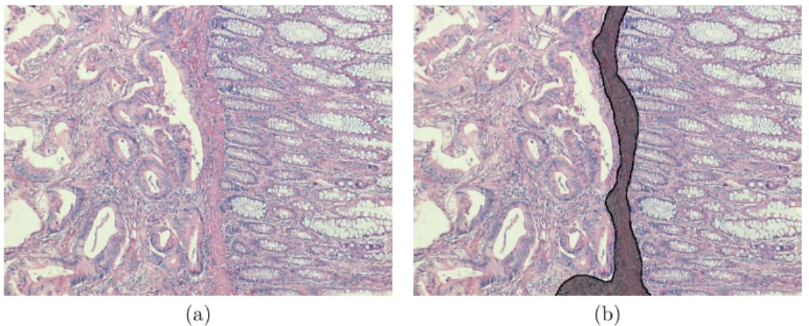
(a) (b)

Figure 3.9: A sample image from SegmentationSet: (a) Original image, (b) gold standard version that indicates homogeneous regions.

six posteriors {πk(pi)}6_k=1 are calculated. According to these posteriors, each

patch is labeled as l(pi) with the class corresponding to the maximum posterior

value.

This initialization phase creates two maps over the image: the first one is the posterior map, Pmap, that is of size m × n × 6 and the second one is the label map,

Lmap, that is of size m × n. Here, m and n are values that depend on parameters,

including patch size (defined by heightP and widthP), image resolution (defined

by heightI and widthI) and overlap distance d. In cases where the combination

of these parameters do not result in a divisible patch number, the last patch takes the respective end points of the image, and encompasses a patch size by taking the necessary number of previous pixels. From this point on, our algorithm works on these maps as they now hold the characterization of all patches. Therefore, when an action is said to be taking place on patches, actually, the action takes place on these maps until the process of remapping which is a part of post-processing (Section 3.2.3). The pseudocode of this initialization phase is given in Algorithm 1.

The next step in our algorithm is seed identification. Here, the aim is to find connected components CC of patches on the image that constitute a homoge-neous region using the constructed maps, that will also be used as a basis for

Algorithm 1 Initialization

Input: Image I, trained CN N , overlap distance d Output: posterior map Pmap, label map Lmap

1: procedure Initialization 2: row ← 0

3: column ← 0

4: while row < heightI do

5: while col < widthI do

6: pi ← I[row : row + heightP − 1, col : col + widthP − 1]

7: {πk(pi)}6_k=1 ← CNNForwardPass(pi) 8: l(pi) = argmax k (πk(pi)) 9: for k = 1 to 6 do 10: P_map(pi, k) ← πk(pi) 11: end for 12: Lmap(pi) ← l(pi) 13: col ← col + d 14: end while 15: row ← row + d 16: end while 17: end procedure

region growing. A pi is selected as a seed patch candidate if it satisfies the

fol-lowing property: The posterior corresponding to its label must be greater than a threshold pthr. The connected components are found on the patch candidates

with the same label and the largest N connected components are determined as initial seeds. This step is detailed in Algorithm 2. The initialization and seed identification steps are illustrated in Figure 3.10.

Algorithm 2 Seed Identification

Input: posterior map Pmap, label map Lmap, number of initial seeds N ,

posterior threshold pthr

Output: initial seeds S

1: _{procedure SeedIdentification}

2: candk ← ∅

3: for k = 1 to 6 do

4: for ∀pi do

5: if Lmap(pi) == lk and Pmap(pi, k) ≥ pthr then

6: candk ← candkSpi 7: end if 8: end for 9: cck ←connectedComponents(candk) 10: CC ← CCS cck 11: end for 12: S ←selectLargest(CC, N ) 13: end procedure

(a) (b)

(c) (d)

Figure 3.10: Illustration of initialization and seed identification steps, on a sample image: (a) Label map (Lmap) of the overlapping patches. (b) Label map when

patches with maximum posterior values smaller than pthr are eliminated. The

eliminated patches are shown with white. (c) Connected components (CC) of the remaining patches. Each connected component is shown with a different color. (d) The N largest connected components. Here, N is selected as 3.

3.2.2

Region Growing

The end product of seed identification step is a collection of seed regions rj,

examples of which are shown in Figure 3.10 (d). The next step is to grow these seed regions over unsegmented regions (which are shown in white in the same figure). To this end, at each iteration, until there is no unsegmented patch to grow upon, all neighboring patches of all grown regions are considered. From

these patches, only one pi is selected for merging into an rj. This pi has the

highest similarity value simpi,rj = Pmap(pi, lrj) where lrj is the class label of the

patches that are initially in region rj (before the growing process takes place).

The pseudocode of the region growing step is given in Algorithm 3, and the operation is visualized in Figure 3.11.

Algorithm 3 Region Growing

Input: seeds S, probability map Pmap, label map Lmap

Output: grown regions R

1: _{procedure RegionGrowing} 2: R ← S 3: for rj ∈ R do 4: lrj ← Lmap( any pi|{pi ∈ rj}) 5: end for 6: while ∃pi|{pi ∈ R} do/ 7: maxsim ← 0 8: for rj ∈ R do 9: for pi|{pi is adjacent to ∃pm ∈ rj, pi ∈ R} do/ 10: simpi,rj = Pmap(pi, lrj)

11: if simpi,rj > maxsim then

12: maxsim ← simpi,rj

13: p∗_i ← pi 14: r_j∗ ← rj 15: end if 16: end for 17: end for 18: r_j∗ ← r∗ j S p∗_i 19: end while 20: end procedure

(a) (b)

Figure 3.11: Illustration of the region growing step, on a sample image. (a) Determined seeds after the seed identification step. (b) Resulting segmentation after the region growing step.

3.2.3

Post-processing

As mentioned, previous steps were carried out on the maps (Pmap and Lmap) that

characterize the overlapping patches. However, due to the overlapping, there is no one-to-one correspondence between this map’s entries and image pixels. Therefore, the first operation that this step accomplishes is the remapping of the segmented map entries back to the image pixels. For this, we use a voting algorithm, where every pi submits a (single) vote in favor of its segmentation

id to all of its pixels. The result is a voting map V, that holds votes for all segmentation ids, for all pixels. When every patch is considered and every pixel’s vote is counted, each pixel is assigned to the segmented region with the highest vote. The result of this remapping procedure (that is applied to the grown regions illustrated in Figure 3.11 (b)) is illustrated in Figure 3.12 (a).

The remapping procedure can produce extra small regions as byproducts (such as the ones indicated by a circle in Figure 3.12 (a)), especially in the region borders. The next procedure therefore in the post-processing step is the clean-up of these small regions. For this, all (now updated by voting) rj are considered. If

the area of a rj is smaller than the area threshold athr, it is merged with its largest

neighbor. Figure 3.12 (b) illustrates the result of this procedure. Notice that there are no small extra regions anymore. This clean-up procedure in post-processing

(a) (b)

Figure 3.12: Illustration of the post-processing step on a sample image: (a) Re-sulting regions after the remapping operation. The circled area includes small regions that are byproducts of the remapping procedure. (b) Resulting segmen-tation after the extra small regions are eliminated by clean-up.

Chapter 4

Experiments

We conduct our experiments on the microscopic histopathological images of colon tissues. We quantatively evaluate our method, comparing its results with those of the others. In this chapter, first, datasets that are used both in the design of our methodology and its evaluation are discussed (Section 4.1). Then, our evaluation technique and metrics are presented (Section 4.2). Next, the methods that we use in comparisons are briefly explained (Section 4.3). Before presenting the results, a discussion is made about the parameters and their selection ranges (Section 4.4). Finally, the results are presented (Section 4.5), followed by a discussion on these experimental results (Section 4.6).

4.1

Dataset

In our experiments, we use two independent datasets: AuxiliarySet, which con-tains patch size annotated homogeneous images, and SegmentationSet, which contains larger unannotated heterogeneous images. In this work, we address the problem of unsupervised segmentation of the heterogeneous images of Segmenta-tionSet. For this aim, we use the supplementary AuxiliarySet in the supervised training/fine-tuning of our convolutional neural network (CNN) model.

(a) (b) (c)

(d) (e) (f)

Figure 4.1: Each image in AuxiliarySet roughly belongs to one of the following categories: (a) Normal, (b) grade 1 cancer, (c) at the boundary between grade 1 and grade 2 cancer, (d) grade 2 cancer, (e) high grade cancer, and (f) medullary cancer.

Both datasets contain microscopic colon tissue images stained with hematoxylin-and-eosin. The biopsies were taken from the Pathology Department Archives of Hacettepe Medical School and their images were acquired by a Nikon Coolscope Digital Microscope. AuxiliarySet contains 900 RGB images acquired by using 20× microscope objective lens. Each image roughly correspond to one of the six categories; containing normal or abnormal formations. An example for each category is given in Figure 4.1. The resolution of these images is 480 × 640. For the usage in Tier 1, these images were cropped (in random positions) to the resolution of 227 × 227, the default input dimension of AlexNet.

The SegmentationSet contains 200 RGB images of resolution 1920 × 2560, acquired by using 5× microscope objective lens. Fifty out of these 200 images were reserved as a training set to estimate method parameters. The remaining 150 were reserved as a test set to evaluate the method’s performance. These heterogeneous images contain both normal and adenocarcinomatous (cancerous) regions of different grades. An example is provided in Figure 4.2. Note that the same training and test sets were used in our previous studies [23].

Figure 4.2: A sample image from SegmentationSet.

The last important point in discussing two sets is their independence. That is, images in AuxiliarySet are not cropped from the larger images of Segmenta-tionSet. This independence is particularly important; because if they were not, the embedded supervised information from Tier 1 would create a positive bias in improving the unsupervised segmentation in Tier 2. Especially, this would result in an (erroneously) improved evaluation, as the segmentation images in that case would not be unseen.

4.2

Evaluation

We quantitatively evaluate the segmentation performance of the proposed deepSeg method using the gold standard versions of the images from SegmentationSet, provided by our medical collaborator. The gold standard versions are delineated by considering the colon adenocarcinoma, which accounts for 90-95% of all col-orectal cancers. This cancer type originates from glandular epithelial cells and

Figure 4.3: Gold standard version of the image shown in Figure 4.2.

causes deformations in colon glands. Non-glandular regions are not important in the context of colon adenocarcinoma diagnosis. Therefore, these regions could be included into either the normal part or the cancerous part. An example is provided in Figure 4.3. In this image, the upper part contains normal regions and the lower one consists of adenocarcinomotous regions. In the middle, which is the shaded part, there exists a region whose characteristics are not important in the context of colon adenocarcinoma diagnosis. Since this thesis focuses on colon adenocarcinoma, such regions will be considered as don’t care regions in the methods’ evaluation.

Our segmentation method, as well as the others used in comparisons, are all unsupervised, so they do not label their segmented regions as normal or cancer-ous. For this reason, for the evaluation, each segmented region rj is attached to

the label of its most overlapping region gk in the gold standard. Then, the

to a cancerous region. If it corresponds to a normal region, these pixels are consid-ered as true negatives (TN). Following the same understanding, non-overlapping pixels of rj are considered as false positives (FP) if gk corresponds to a cancerous

region, and they are considered as false negatives (FN) if gk corresponds to a

normal region. The pixels of the don’t care region in the gold standard are not considered in this evaluation. Using these four numbers, four evaluation metrics are calculated: accuracy, sensitivity, specificity, and f-score; whose definitions are given in the following equations.

accuracy = (T P + T N )/(T P + T N + F P + F N ) (4.1)

sensitivity = T P/(T P + F N ) (4.2)

specificity = T N/(T N + F P ) (4.3)

precision = T P/(T P + F P ) (4.4)

recall = T P/(T P + F N ) (4.5)

f-score = 2 × (precision × recall)/(precision + recall) (4.6)

4.3

Comparisons

In order to compare our results with those of the others, we use the following five methods: MLSeg [23], graphRLM [22], objectSEG [21], graph-based segmentation (GBS ) [32], and J value segmentation (JSEG) [33]. The first three are the ones that were previously developed in our research group for the specific purpose of tissue segmentation. These algorithms all decompose an image into a set of circular objects. They then define handcrafted textural features on these objects to quantify their spatial distribution and use these handcrafted features in the segmentation. The comparison of the proposed deepSeg with these algorithms enables to understand the effects of using deep learning based features instead of the handcrafted ones.

The GBS and JSEG algorithms are known as effective general-purpose seg-mentation algorithms, so they are not specially designed for segmenting tissue images. These algorithms also employ handcrafted features for segmentation. The comparison with these two methods enables to understand the importance of using domain specific knowledge (which we introduce in Tier 1, when we fine-tune our model using tissue images), as well as observe the effects of using deep learning based features. The details of these five algorithms are given below.

• Multilevel segmentation (MLSeg) algorithm: A tissue image is decomposed into a set of circular tissue objects, which approximately represent tissue components. Then the object cooccurence features are extracted on these objects by calculating the frequency of cooccurrence of two object types with different distances. Consequently, a weighted graph is constructed between the objects where an edge in between two objects corresponds to the similarity between the features of these objects. Finally, a multilevel graph partitioning algorithm is used on this graph to obtain the segmentation [23].

• Graph run-length matrix (graphRLM ) algorithm: Similarly in this algo-rithm, an image is decomposed into tissue objects. Then, a graph is con-structed on these objects and its edges are colored according to their end-points. Using these colored edges, a run length matrix is generated on this graph. The features extracted from this run length matrix are used in a region growing algorithm to obtain the segmentation [22].

• Object oriented segmentation (objectSEG) algorithm: This method also defines circular tissue objects and defines two uniformity measures on these objects. These are the object size uniformity and object spatial distribution uniformity, which quantify how the objects are distributed in size and space, respectively. Then those features are used in a region growing algorithm to segment a tissue image [21].

• Graph-based segmentation (GBS ) algorithm: This method constructs a graph on an image, where the nodes are pixels and the edges are the dis-similarity values between the pixels (based on their properties)– with the

overall aim of obtaining low dissimilarity values among the elements in a component, and high dissimilarity values in different components. Based on this predicate, this method uses a greedy algorithm for segmentation [32].

• J value segmentation (JSEG) algorithm: This two-stage method accom-plishes color quantization in the first phase to create a label map of an image. Then, according to a defined spatial criterion J on good segmenta-tion, this method minimizes this criterion in the second phase. For that, it first reconstructs the image based on local J values as pixel values. Then, it performs a region growing algorithm on this reconstructed image by the steps of seed determination, seed growing, and region merge to obtain the segmentation [33].

4.4

Parameter Selection

The first tier of our method contains the hyper-parameters of the used convolu-tional neural network (CNN) model. Its second tier has the parameters related with the seed-controlled region growing algorithm. These parameters and their selected values are explained in the following subsections.

4.4.1

Parameters of Tier 1

We use transfer learning to fine-tune the AlexNet model in Tier 1. If we use a new model, we would need to make decisions for all aspects related to the CNN. This includes, but is not limited to the number and types of layers, the kernel sizes, pads and strides for convolutional and pooling layers, the number of outputs that convolutional and fully connected layers produce, and nonlinearity, pooling operation types– essentially every parameter discussed in Section 2.1. In the context of learning algorithms, these parameters are called hyper-parameters. More formally, a hyper-parameter set is a set H of parameters, which must be chosen (not derived) in order to obtain the actual learning algorithm [34].

In our case however, as we decide to use transfer learning (mainly due to the limited nature of our dataset) on the exact AlexNet model, only model’s size related hyper-parameter that must be altered is the last fully connected (decision) layer’s number of outputs, which is updated as six to correspond to the number of classes represented in AuxiliarySet, so there is no need for a selection. We use the AlexNet model as it is (except its last layer) because of the following reasons. Due to the similarities of our image scales, we do not want to leave out, replace or add any layers, with the logic that a model that has appropriate depth, width and layer properties to fairly learn an image dataset should not fail to learn a different dataset that consists of images which are similar in resolution. Therefore, instead of substantially modifying AlexNet, we crop our AuxiliarySet images at random positions to meet the ImageNet input size. This usage also enables us to transfer the maximum possible amount of information, from the unmodified layers of AlexNet. The rationale for using AlexNet architecture rather than a variation is validated when the evaluation results are presented for multiple models (Section 4.6).

However in fine-tuning, we had to consider the differences of both datasets– ImageNet and our histopathological tissue image dataset, and selected the learn-ing parameters to successfully learn our dataset. We use five learnlearn-ing parame-ters in defining the training operation. These are the base learning rate baseη,

learning rate multiplier γ, learning rate update stepsize S, total number of iter-ations numiter, and momentum α. The selected values of these parameters are:

baseη = 0.001, γ = 0.8, S = 2000, numiter = 15, 000, and α = 0.9. These

param-eters are mainly selected by trial-and-error. When a parameter set was selected, the training is allowed to continue for a limited time. At that time, the changes in the error function output and validation images’ accuracy are observed. If the change is satisfactory, meaning that the classification error is decreasing in a desirable rate, the iterations are allowed to continue. These parameters are taken from the best such operation. Here, note that the validation images are also selected among AuxiliarySet, so SegmentationSet images that are used for evaluation are not used at all. Similarly, the rationale of using transfer learning rather than learning from scratch is validated when the evaluation results of both