TESTING CAUSAL RELATIONSHIPS BETWEEN
ENERGY CONSUMPTION, REAL INCOME AND
PRICES: EVIDENCE FROM TURKEY
C e m S A A T g i O G L U1 H. Levenl K O R A P
ÖZET
Bu çalışmada, enerji tüketimindeki değişimler, ıtel gelir büyümesi ve yurtiçi enflasyon arasındaki nedensellik ilişkileri Türkiye ekonomisi koşullarında araştırılmaktadır. Çağdaş çok değişkenli eş-bütünleşim tahmin yöntemi kullanılarak elde ettiğimiz bulgular, enerji tüketiminin araştırılan nedensellik ilişkilerinin aydınlatılabilmesi için, çeşitli kategorilere ayrıştırılması gerektiğini göstermektedir. Vurgulanması gereken temel bulgularımız, yurtiçi enflasyonıst yapının oluşturulan modeller için oldukça içsel bir yapıya sahip ve özellikle enerji tüketimindeki değişikliklere karşı duyarlı ve sanayi tüketimi uygun enerji tüketim verisi olarak dikkate alındığı zaman, nedensellik çözümlemesi içerisinde birbirlerine karşı oldukça içsel bir yapıda tahmin edilen değişkenlerin uzun dönemli bir nedensellik ilişkisi içerisinde oldukları şeklinde belirtilebilir. Sonuç olarak, l>eklentiler doğrultusunda tasarlanan enerji politikalarının ekonomi içerisinde belirleyici bir şekilde yurtiçi enflasyonu etkileme gücüne sahip olduğu v e ev halkının kullanım amacına yönelik ya da ticari içerikli enerji tüketiminin, toplam enerji tüketiminden ziyade sanayi enerji tüketimi dikkate alındığı zaman, enerji tasarruf politikalarının reel gelir büyüme süreci açısından zararlı olabilecek sonuçlar meydana getirebileceği görülmektedir.
Anahtar Kelimeler: Enerji Tüketimi; Reel Cici ir; fiyatlar; Nedensellik; Türkiye Ekonomisi; JEL sınıflaması: G 2 ; E31; Q43;
ABSTRACT
Jıı this paper, w e examine the causal relationship amongst changes in energy consumption, real income growth and domestic inflation within the conditions of Turkish economy. Based on a contemporaneous multivariate co-integrating estimation methodology, our estimation results indicate that a distinction between various categories of enei'gy consumption needs to l>e made in order for the causality issues of interest to be elucidated. We find as a vital point to be emphasized that domestic inflationary framework is highly endogenous to all the model constructions and thus subject to the changes in especially enei'gy consumption. It is also significant that there seems to be a long-ran causal relationship between the variables when the levels of industrial consumption are used as the relevant enei'gy consumption data since they have highly endogenous characteristics against each other within the causality analysis. We conclude that energy policies ex-ante designed have the power of affecting domestic inflation significantly. We also suggest that, for the case of industrial energy consumption data, energy conservation policies may lead to harmful results for the real income growth process though the latter issue is not the relevant case for the residential and commercial enei'gy consumption and total enei'gy consumption data. R e w o r d s : Enei'gy Consumption; Real Income; Prices; Causality; Turkish Economy; J e L classification: 0 2 ; E31; Q43;
' Ass. P r o f , Istanbul University f a c u l t y and Department of Economics, sa ate i c fe? i sta n hu 1. edu ,tr * Economist. Marmara University, korap ko 1 a v. net
Evidence I r o m Turkey
1. INTRODUCTION
One of the main controversial issues of interest in contemporaneous economics policy debates is to detect the causal relations among energy consumption and economic growth. This has been of special importance for policy makers since both the temporal causality and the knowledge of a possible stationary relationship relating energy consumption and economic growth to each other would have significant implications in policy design and implementation process so as to assess the long-run course of the energy policies within developed as well as developing countries. If a uni-directional causality can be attributed to the energy consumption and economic growth relationship, running from the latter to the Conner, this would mean that no signilicant adverse-causal effect of energy conservation policies must be expected on economic growth. On the other side, if such a causality runs Irorn energy consumption to economic growth, policies aiming at reducing energy consumption may deteriorate the real income growth process since this indicates the energy-dependent characteristic of the economy. If no causality is found between energy consumption and economic growth, referred to as
neutrality hypothesis due to Yu and Choi (1985), this impli es that energy
consumption is not correlated with economic growth, and energy conservation policies may be pursued without adversely affecting the economy (Jumbe, 2004). Therefore, the relations between energy consumption and economic growth are deserved to be examined elaborately and inferences which can be drawn from these analyses would enable policy makers to carry out appropriate energy policies
In this paper, our aim is to examine the long- and the short- run causal relations between the changes in energy consumption represented by electric power consumption, real income growth and domestic inllation in the Turkish economy. For this purpose, the next section gives a large literature review and the third section briefly highlights some stylized facts of the Turkish economy.
The fourth section examines some preliminary daia issues and ihe fifth section discusses some econometric methodological issues to be applied for empirical purposes. The sixth section conducts an empirical model upon the Turkish economy and linally the last section summarizes results, gives policy implications, and concludes.
2. LITERATURE REVIEW
Following the energy crises occured in the 1970s, there has been an extensive research area on the energy consumption - economic growth relation for various country
cases. The literature constructed on this issue of interest follow clearly the developments in modem time series estimation techniques to reveal the extent to which causality is attributed and to examine the direction of this relationship. The seminal paper by Kraft and Kraft using Sims causality tests (1978) find a uni-directional causality running from gross national product (GNP) to energy consumption for the US economy over the period 1947-1974. However. Akarca and Long (1980) indicate that the results in Kraft and Kraft (1980) suffer Iroin temporary sample instability affecting the estimation results when the data sample is shortened. Yu and Hwang (1984) also using US data for the 1947-1979 period estimate no causal relationship between energy consumption and GNP supporting the so-called neutrality hypothesis. Yu and Choi (1985) using Granger causality tests examine such a relationship for a group of countries and lind a causality from GNP to energy consumption for South Korea and Irom the latter to the Conner for Philippiness over the period
1954-1976. while no causality is observed Cor the cases of US, UK and Poland. Erol and Yu (1987) using Sims and Granger causality tests Cind uni-directional causality from energy consumption to income Cor West Gennany, bi-directional causality Cor Italy and Japan and no causal relations Cor UK, Canada and France. Yu and Jin (1992) investigating integration and co-integration properties of energy consumption against industrial output and
Evidence I r o m Turkey
employment lor the US over the period 1974-1990 reveal no long-run stationary relationship between the variables and give support to the neutrality hypothesis lor energy consumption.
Masih and Masih (1996) and Masih and Masih (1998) examine the relation between total energy consumption and real income for a group of Asian economies over the period of 1955-1991. They find no causal relation for Malaysia, Singapore, and Philippines, a uni-directional causality Irom energy consumption to GNP lor India, Sri Lanka and Thailand, a reverse causal relationship lor Indonesia, and a mutual causality for Pakistan. Masih and Masih (1997) also test lor co-integration between total energy consumption, real income and price level lor Korea and Taiwan. Their results using multivariate co-integration and vector error correction (VEC) approach as well as considering some decomposition and impulse-response tests indicate that there exists a jointly interactive causal chain between the variables in line with the estimation results of Hwang and Gum (1992) yielding bi-directional causality between income and energy in Taiwan. Glasure and Lee (1997) examine the causality issue between energy consumption and gross domestic product (GDP) lor South Korea and Singapore with the aid of co-integration and error correction modeling over the period of 1961-1990 and lind a bi-directional causality between GDP and energy consumption. Likewise, Hondroyiannis et al. (2002) using Greece data over the period of 1960-1996 support the endogeneity of energy consumption and real output and emphasize the existence of a bi-directional relationship between these variables. Asal'u-Adjaye (2000) employing a vector error correction methodology estimates that considering the period of 1973-1995 there exists uni-directional short-run causality running Irom energy to income Cor India and Indonesia, while bi-directional Granger causality runs from energy to income for Thailand and Philippines. Soytas and Sari (2003) re-examine the causal relationship between GDP and energy consumption Cor the top ten emerging markets except China
and lor G-7 countries. They discover bi-directional causality in Argentina and causality from energy consumption to GDP in Turkey. France. Germany and Japan, which is attributed to that energy conservation may harm economic growth lor these countries. They also find that the causal relation appears to be reversed lor Italy and Korea.
Based on a production function approach considering output, capital, labor and energy use. Ghali and Sakka (2004) also analyze the causal relations between energy use and output growth in Canada for the period 1961-1997. They indicate that energy enters significantly the long-run stationary relationship constructed between these variables. Moreover, a bi-directional causality between output growth and energy use is found. Oh and Lee (2004) construct demand and production side models using a VEC model to investigate the causal relations between GDP and energy for Korea and find a uni-directional causality running from GDP to energy in the long-run. Following the estimation results obtained, they emphasize that energy conservation policy may be feasible without compromising economic growth in the long-run.
Finally, employing recently developed panel unit root and heterogeneous panel causality and co-integration tests, Lee (2005) investigate co-movement and causality relationship between energy consumption and GDP in 18 developing countries for the period 1975-2001. Results indicate that long- and short-run causalities run from energy consumption to GDP leading to the conclusion that energy conservation may harm economic growth in developing countries. However, Al-Iriani (2006) using data Irom the countries of Gulf Cooperation Council (GCC) and Mehrara (2007) using data from 11 oil exporting countries through panel estimation techniques indicate a uni-directional causality from GDP to energy consumption and suggest that energy conservation policies may be adopted without much concern about their adverse effects on the economic growth. Thus, no clear-cut inference can be
Evidence I r o m Turkey
drawn about the causal relations between energy consumption and real income, and this relation is highly sensitive to the time periods and estimation techniques employed lor empirical purposes even lor the same country cases.
3. SOME STYLIZED FACTS FROM THE TURKISH ECONOMY
As a developing country, a cursory examination of the courses of both economic growth and electric energy consumption, and also dividing this relation as to the sub-periods and sub-components lor the Turkish case are able to yield some stylized facts of the economy. In Tab. I below, we give some knowledge of electric power consumption and economic growth in the Turkish economy:
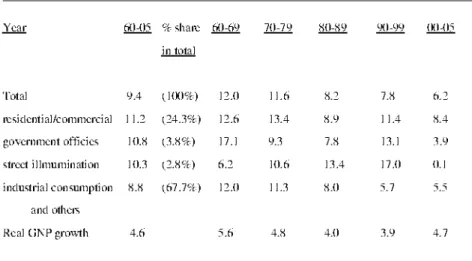
Table 1. Electric Consumption and Real GNP Growth
(10-years average of annual per cent growth rates for the sub-periods)
Year 60-0? % share 60-69 70-79 80-89 90-99 00-05 in total Total 9.4 (.100%) 12.0 11.6 8.2 7.8 6.2 resident ial/commcrci al 1 1.2 (24.3%) 12.6 13.4 8.9 1 1.4 8.4 government officies 10.8 (3.8%) 17.1 9.3 7.8 13.1 3.9 street illmumination 10.3 (2.8%) 6.2 10.6 13.4 17.0 0.1 industrial consumption 8.8 (67.7%:) 12.0 11.3 8.0 5.7 and others Real GNP growth 4.6 5.6 4.8 4.0 3.9 4.7
Source: Statistical Indicators 1 923-2(X)5. Prime Ministry Republic of Turkey Turkish Statistical Institute. T h e relative shares of sub components of the total electricity power consumption growth rates may not lie summed to 100% due to rounding problems.
In Tab. 1 above, we see that the Turkish economy has been subject to a 4.6% annual real income growth rate for the 1960-2005 whole period. However, there exist some fluctuations in the growth rates as to the sub-periods in the
sense that ihe 1960s and 1970s have an average of about 5% or higher annual average growth rates, while the 1980s and 1990s witness a substantial drop to the 4% in the growth rates. There seems to be a revival in the real income growth rates lor the post-2000 period, which has an annual real income average growth rate of 4.7%. The course of total electricity power consumption data coincides somewhat with the real income growth rates. We can easily notice that the 1960s and 1970s have the largest growth rates in the total electricity consumption and these growth rates even exceeds considerably real GNP growth rates indicating the pace of industrialization as well. But substantial drops in the energy use growth rates occur in the 1980s and 1990s such as the drops in real income growth rates. The two main items in the total electricity energy use are the residential plus commercial and the industrial consumption data, lor which the latter dominates the total electricity consumption and has highly similar trends to the total consumption. The shares of other two items in the total electricity use, i.e. the shares of government offices and street illumination, take highly trivial values so that we will omit below these latter items in our empirical model estimation.
4. PRELIMINARY DATA ISSUES 4.1. Data
We now test for the existence of a potential long-run stationary relationship between energy consumption and real income for the Turkish economy. Following Masih and Masih (1997) and Hondroyiannis et al. (2002), we consider the effects of prices on this relationship as well. Hondroyiannis et al. (2002) attribute the inclusion of prices into the energy consumption - real income relationship to that prices would represent a proxy for the efficient functioning of the economy and that such an inclusion may reveal the role of prices in affecting the use of energy especially for a developing country such as Turkey. Thus prices may provide us the knowledge of whether energy
Evidence I r o m Turkey
policies can affect the efficiency and the lechnological progress in the economy.
In Tab. 1, we see that the two main components in the total energy consumption are residential-commercial energy consumption and industrial consumption. To examine the sensitivity of the results, we therefore analyse the relationship between energy consumption and real income as to these sub-consumption categories separately. The empirical model is carried out for the investigation period of 1968-2005 of 38 annual observations. The real income variable (Y) is represented by real gross national product (GNP) data at 1987 constant prices. For the energy consumption data, we use total energy consumption (TOT), residential and commercial energy consumption (RC) and industrial consumption (IND), while GNP-dell at or (DEF) is considered for the relevant price variable. All the data are taken from the Statistical Indicators
1923-2005 published by the Prime Ministry Republic of Turkey Turkish Statistical Institute and are in their natural logarithms. Besides, we include three impulse-dummy variables into the model specilication as exogenous variables which take on values of unity for the years 1980, 1994 and 2001 concerning the financial crises and the political breaks and instabilities overwhelming the Turkish economy.
Unit Root Characteristics
We now investigate the time series properties of the variables. Spurious regression problem introduced by Yule (1926) and further analysed by Granger and Newbold (1974) indicates that using non-stationary time series steadily diverging Irom long-run mean will produce biased standard errors, which causes to unreliable correlations within the regression analysis leading to unbounded variance process. In this way, when a non-stationary 1(d) process identifies any time series, the standard OLS regression in the level form will possibly produce a good lit and predict statistically signilicant relationships between the variables where none really exists (Mahadeva and Robinson,
2004). This means ihai the variable must be differenced (d) limes to obtain a eovarianee-stationary process. Therefore, individual time series properties of the variables should be elaborately considered. Dickey and Fuller (1979. 1981) provide one of the commonly used test methods known as augmented Dickey-Fuller (ADF) test of detecting whether the time series are of stationary form. This can be formulated such as:
A
AX, = a + pi + (p-l)X,, + ^ , , • + £ , (1)
1=1
of which ihe null hypothesis is the presence of a unit root (p=l) against the alternative stationary hypothesis. For X, to be stationary, (p-1) should be negative and significantly different Irom zero. We compare the estimated ADF statistics with the simulated MacKinnon (1991, 1996) critical values, which employ a set of simulations to derive asymptotic results and to simulate critical values for arbitrary sample sizes. We expect that these statistics must be larger than critical values in absolute value and have a minus sign.
Besides the conventional ADF test in Eq. (1), Elliot et al. (1996) propose a more powerful modified version of the ADF test in which the data are detrended so that explanatory variables are taken out of the data prior to running the test regression. Elliot et al. (1996) define a quasi-difference of X, that depends on the value a representing the specific point alternative against which we wish to test the null. Following QMS (2004), we can write down:
X, i f i = 1
d(X, | a ) = (2) X, - otX, i if t > 1
An OLS regression of the differenced data d(X, | a ) on the quasi-differenced d(Z, | a ) yields:
d(X, | a ) = d(Z, | a)'8(a)+r), (3)
Evidence I r o m Turkey
where Z, consists of deterministic constant or constant and trend terms and let 8(a) be the estimated value from an OLS regression. For the value of a, Elliot et al. (19%) consider:
1 - 7 / T i ! ' Zt= { l }
a = (4) 1 - 13.5/T iI Z, = {l.t}
Following these specification issues, generalized least squares (GLS) deirended d a t a X / are:
Xtd = X, - Zt'5i a ) (5) The DFGLS substitutes the GLS detrended Xtd data lor the original Xt data in
Eq. 1 above. While the DFGLS t-ratio follows a Dickey-Fuller distribution in the constant only case, the asymptotic distribution differs when included both a constant and trend. Elliot et al. (1996) simulate the critical values of the test statistic in this latter setting f o r T = (50, 100, 200, M}.
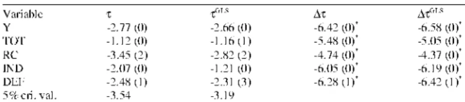
For the MacKinnon critical values, we consider 5% level critical values for the null hypothesis of a unit root. The numbers in parantheses are the lags used for the ADF stationary test and augmented up to a maximum of 8 lags. The choice of the optimum lag for the ADF and DFGLS tests was decided on the basis of minimizing the Schwarz information criterion. For all the unit root tests, we report below in Tab. 2 the results with a linear time trend in the test equation:
Table 2. Unit Root Tests
Vari ah] e t •t™ A t A t ™ Y -2.77 (0) -2.66 (0) -6.42 (0)* -6.58 (0)* t o r - 1 . 1 2 ( 0 ) - 1 . 1 6 ( 1 ) -5.48 (0)* -5.05 (0)* R C -3.45 (2) -2.82 (2) -4.74 (0)* -4.37 (0)* IND -2.07 (0) -1.21 (0) -6.05 (0)* -6.19 (0)* DEI'' - 2 . 4 8 ( 1 ) -2.31 (3) -6.28 ( ] ) ' -6.42(1)* 5 % c r i . val. -3.54 -3.19
Above, T and Tg l s arc the icsi statistics with allowance lor constant and trend terns in the ADF and DFf'LS unit root tests, respectively. 'A' denotes the first difference operator, while ' means that the data are of stationary form. For all the variables, the null hypothesis that there is a unit root cannot be rejected. From now on. we thus assume that all the variables are difference-stationary, and that they are integrated of order 1. i.e. 1(1). which have an invertible ARMA representation after applying to lirst differencing.
5. ESTIMATION METHODOLOGY 5.1. Meaning of Co- Integration
The classic paper by Nelson and Plosser (1982) reveals that many macroeconomic time series data have a stochastic trend plus a stationary component, that is. they are difference stationary processes, and as Enders (2004) stated numerious economic theories suggest the importance of distinguishing between temporary and permanent movements in a series. Besides, economic theory assumes that at least some subsets of economic variables do not drift through time independently of each other and some combination of the variables in these subsets reverts to the mean of a stable stochastic process (Anderson et al., 1998).
In this sense. Granger (1986). Engle and Granger (1987) and Granger (1988) indicate that even though economic time series may be non-stationary in their level forms, there may exist some linear combination of these variables that converge to a long run relationship over time, which also requires that there must be Granger causality in at least one direction in an economic sense as one variable can help forecast the others. That is, if the series are individually stationary after differencing but a linear combination of their levels is stationary then the series are said to be co-integrated. In such a case, they cannot move too far away from each other in a theoretical sense (Dickey, Jansen and Thornton, 1991).
Evidence I r o m Turkey
Therefore, error-correcliori modeling derived from a co-integration analysis enables researchers to track both short- and long- run dynamics between the variables in the long-run variable space and provides long-run stability by the introduction of error correction term in order to adjust for departures from equilibrium. Otherwise, by analysing only the differences of economic time series all information about potential long-run relationships between the levels of economic variables would be lost (Hendry, 1986). Contemporaneous co-iniegration techniques, e.g. proposed by Johansen (1988) and Johansen and Juselius (1990) as a further development to co-integration methodology, which enables researchers to test that more than one stationary long-run equilibrium relation can be lying in the long-run variable space, take account of the non-stationariiy characteristics of the most economic aggregate time series. Whereas, employing conventional estimation techniques based on an OLS estimation would not possibly lead to a constant mean and a linite variance and therefore diverge after a shock. In line with these developments in econometrics theory, contemporaneous economic theories make use of these estimation tools in constructing and testing the theories based on model specilication issues conditioned upon econometrics.
5.2. J oh an sen-Juselius Co-Integration Methodology
In order to test for a stationary relationship among the variables for empirical purposes in our paper, we apply to the multivariate co-integration and vector error correction (VEC) techniques proposed by Johansen (1988) and Johansen and Juselius (1990) and search for whether it is possible to extract any steady-state knowledge from the long-run variable space. Gonzalo (1994) indicates that this method performs better than other estimation methods even when the errors are non-normal distributed or when the dynamics are unknown. This methodology constructs an error correction mechanism among the same order integrated variables, which enables that a stationary combination of the variables do not drift apart without bound even though all have been
individually subject ıo a non-sıaıionary 1(d) process, therefore ruling out the possibility that estimated relationships tend to be spurious. Besides, this technique is superior to the regress i on-based techniques, e.g. Engle and Granger (1987) two-step methodology, for it enables researchers to capture all the possible stationary relationships lying within the long-run variable space.
Let us assume a z, vector of non-stationary n endogenous variables and model this vector as an unrestricted vector autoregression (VAR) involving up to k-lags of z,:
z, = Hi z, +
n
2z,
2+...
+
n
kz,
k + e, (6)where et follows an i.i.d. process N(0, c2) and z is (nxl) and the n i an (nxn) matrix of parameters. Eq. 6 can be rewritten leading us to a vector error correction (VEC) model of the form:
Az, = F|Az, | + r2Az, 2 + ... + rt |Az, t+1 + üz, t + £, (7)
where:
r, = -i + n , + ... + i l (i = i, 2, ...,k-i) and n = i - n , - n2 ... nk (8) Eq. 7 can be arrived by subtracting z,-i Irom both sides of Eq. 6 and collecting terms on z, ı and then adding -(H| - 1)X, ı + (H| - 1)X, Repeating this process and collecting of terms would yield Eq. 7. This specilication of the system of variables carries on the knowledge of both the shon- and the long-run adjustment to changes in z,. via the estimates ol' T, and n . Following Harris (1995). n = a|i' where a measures the speed of adjustment coefficient of particular variables to a disturbance in the long-run equilibrium relationship and can be interpreted as a matrix of error correction terms, while (3 is a matrix of long-run coefficients such that p'z, k embedded in Eq. 7 represents up to
(n-1) cointegrating relations in the multivariate model which ensure that z, converge to their long-run steady-state solutions. Note that all terms in Eq. 7 which involve Az, i are 1(0) while FIz, k must also be stationary for e, ~ 1(0) to be white noise of an N(0. c( 2) process.
Evidence I r o m Turkey
As a next step, we estimate the long run eo-integrating relationships between the variables by using two likelihood test statistics known as maximum eigenvalue lor the null hypothesis of r versus the alternative of r+1 eo-integrating relationships and traee lor the null hypothesis of r eo-eo-integrating relations against the alternative of n eo-integrating relations, lor r = 0,1, ... ,n-l where n is the number of endogenous variables. Following Johansen (1992), lor the co-integration test we restrict intercept and linear trend factors into our long run variable space in line with so-called Pantula principle. This requires a test procedure which moves through from the most restrictive model and at each stage compares the trace or max-eigen test statistics to its critical value and only stop the first time the null hypothesis is not rejected. Doornik et al. (1998) also indicate that restricting the trend factor into the co-integration space is preferable. However, we give the estimation results below with the case of unrestricted trend in the co-integration analysis for comparison purposes.
5.3. Causality Analysis
We will test the possible causality relationships between change in energy consumption, real income growth and domestic in 11 a don data through the Granger causality tests considering also the knowledge of co-integrating relationship included into the causality analysis. In this way, we examine both the long-run causality captured by the significance of the error-correction term and the short-run causality derived by testing the signilicance of sum of the lags of explanatory variables. If we write down the variable system in a VEC form:
n n n r
AY, = +Ey.MAXti + £r|-MAYt , + IKMADEF, , + D^ECT,., + £1t (9)
i=l i=l i=l i=l
n n n r
AX, = ()>,+ £y2lAX,, + Ir|2lAY, , + IK2IADEF, , + IX2IECT,„ , + £2, (10)
i=l i=l i=l i=l
ri ri ri r
ADEF^ifi, +Ly; iAXt l + Lr|;iAYtl +lK; iADEFt l +LX; iECTl ? t, + (11) i=l i=l i=l i=l
where Y, is the real income. X, ihe energy consumption data which represent either total energy consumption or residential and commercial energy consumption or industrial consumption, and DEF, the relevant GNP-dellator data, n is the choosen lag length lor the order of autoregressive models and £,./s lor i = 1.2.3 are disturbance terms assumed whitening the error structure of the models with a N(0. of 2) process. ECTs stand lor the error correction terms taken Irom long-term co-integrating space.
Eqs. 9-11 are used below to evaluate the causality analysis between changes in energy consumption, real income growth and domestic inflation. In Eq. 9 we search lor whether there exists a causal relationship running Irom change in energy consumption and domestic inflation to the real income, while in Eq. 10 and Eq. 11 causal relationships running from real income growth and domestic inflation to the changes in energy consumption and also running Irom real income growth and changes in energy consumption to the domestic inflation are c on si d ered. re spec ti v e 1 y.
Error correction mechanisms included in the autoregressive models given above provide researchers additional knowledge of causal relations between the variables ignored by the initial Granger (1969) and Sims (1972) tests, which allow to distinguish short- and long-run causality from each other. The Wald- or F-tests applied to joint significance of the sum of the lags of each explanatory variable and the t-tests of the lagged error correction terms will highlight us for the knowledge of Granger exogeneity or endogeneity of the each dependent variable in a statistical sense. If the dependent variables can be driven by the error term yielded in the stationary co-integrating vector, which explains speed of feedback effects towards the long-term steady-state
Evidence I r o m Turkey
relationship correcting short-term dynamic disequilibrium conditions, this implies the existence of a long-run causal relationship. Such a finding is equivalent to say that the variable considered has not been found weakly exogenous with respect to stationary co-intagrating variable space. This can be done by testing H,,: Xtl = 0 through t-tests of the lagged error correction terms. If the non-significance of the error correction terms is accepted, this means the dependent variable responds only to short-term shocks to the stochastic environment (Masih and Masih, 1997; Oh and Lee, 2004). In this sense, the rejection of the non-significance of differenced explanatory variables by the Wald- or F-tests will be referred to as short-term causality. This can be done by testing the null hypothesis of the non-signilicance of yti, T|ti or k, in Eqs.
9-11 through Wald- or F-tests. Finally, we test jointly non-significance of all the explanatory variables including both differenced-stationary variables and the lagged error correction terms in the VEC mechanism for the absence of Granger causality, that is what Hondroyiannis et. al. (2002) call "strong exogeneity of the dependent variable".
6. RESULTS
We report first below the estimation results for the co-integrating rank test between energy consumption, real income and general price level. For the energy consumption, we take into account these relationships separately as for the total energy consumption, residential and commercial energy consumption and industrial consumption data. The lag length of the unrestricted vector auioregressive (VAR) models upon which co-integrating models, if any, are tried to be constructed is determined by using five lag order criterions i.e., sequential modified LR statistics employing small sample modification, minimized Akaike information criterion (AIC), final prediction error criterion (FPE), Schwarz information criterion (SC) and Hannan-Quinn information criterion (HQ) to select appropriate model between different lag specifications. Considering the maximum lag of four for the unrestricted VAR models of
annual observations, all the eriterions suggest to use two lag orders lor three models using different energy consumption data. The rank test results are given in Tab. 3 below, denotes rejection of the hypothesis at the 0.05 level:
Table 3. Co - Integration Rank Tests
Model 1 no linear trend restricted linear trend restricted
T O T - Y - D E E Null hypothesis r=<) i<] i<2 r=0 I<1 i<2
Eigenvalue 0.43 0.25 0.01 0.51 0.42 0.11
X trace 29.93* 10.04 0.02 4 8 . 2 3 23.29 4 . 2 2
5 % cri. val. 29.80 15.49 3.84 42.92 25.87 1 2.52
X max 19.89 10.01 0.02 24.94 19.07 4.22
5% cri. val. 21.13 14.26 3.84 25.82 19.39 12.52
Model 2 no linear trend restricted lineartrend restricted
R C - Y - D E E Null hypothesis 1^0 |<1 i<2 1^=0 I<1 i<2 Eigenvalue 0 . 5 8 0 . 2 8 0.02 0.65 0 . 4 8 0.16
X trace 42.82* 12.20 0.55 65.13' 28.87' 6.19
5 % cri. val. 29.80 15.49 3.84 42.92 25.87 12.52
X max 30.62* 1 1.65 0.55 36.25' 22.68' 6.19 cri. val. 21.13 14.26 3.84 25.82 19.39 12.52
Model 3 no lineartrend restricted lineal' trend restricted
JND-Y-DEI Null hypothesis r=0 i<] i<2 r=0 I < 1 i<2
Eigenvalue 0.40 0.25 0.01 0.59 0.36 0 . 0 8
trace 28.11 10.44 0.22 49.48' 18.49 2.90
5 % cri. val. 29.80 15.49 3.84 42.92 25.87 12.52
X max 17.67 10.22 0.22 30.99* 15.59 6.19
5 % cri. val. 21.13 14.26 3.84 25.82 1 9.39 12.52
In Tab. 3 above, we find that there exists a stationary long-run relationship through the trace-test statistics between total energy consumption, real income and general price level when we do not restrict the trend factor into the long-run variable space. Likewise, for the Model 3 the null hypothesis of no co-integration can be rejected in favor of one co-integrating vector but now assuming a restricted deterministic linear trend factor in the co-integrating space. Finally, the rank test results for Model 2 reveal that two potential stationary vectors lie in the variable space. It is not uncommon to find more than one co-integrating relationship in a system with more than two variables using Johansen procedure. In this case, we choose to consider the
Evidence I r o m Turkey
integrating vector which yields the largest eigenvalue in order to avoid the identification problems occuring when the cointegrating rank r>l. Otherwise, following Harris (1995). what the reduced rank regression procedure provides is information on how many unique integrating vectors span the co-integration space, while any linear combination of the stationary vectors is itself a stationary vector. In that case, the estimates produced for any particular column in p would not be necessarily unique, which requires the identilication of each vector in line with economics theory or arbitrarily by imposing restrictions to obtain unique vectors lying within that space. Considering these difficulties and to avoid imposing any arbitrary identification restriction for the second potential vector, we follow for the case of Model 2 the first vector with the largest eigenvalue. Besides, we estimate Model 1 by assuming no deterministic linear trend lying in the long-run variable space, but due to the Pantula principle expressed above and following Johansen (1992) we estimate Model 2 and Model 3 by restricting a deterministic linear trend in the co-integration analysis.
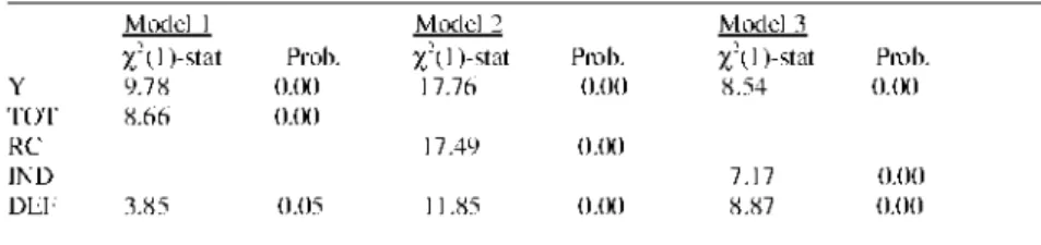
Under the assumption o f r = 1, we can easily notice in Tab. 4 below that all the variables have statistical significance and belong to the relevant integrating relationship by using zero restriction LR tests on the long-run co-integrating coefficients:
Table 4. Significance of Co-Integrating Coefficients
Model 1 Model 2 Model 3
)-stat Proh. % \ l )-stat Proh. )-stat Proh.
Y 9.7 X (UK) 17.76 0.00 8.54 <).<K)
t o r 8.66 (UK)
R C 17.49 ().(K)
IND 7.17 0.00
DEI; 1 X 5 0.05 11.85 ().(K) 8.87 0.00
In Tab. 4, we find that both real income, energy consumption and general price level data enters the co-integrating vectors in a statistically significant
way. For ihis purpose, we assume chi-square i'/J) lesi siaiisiies using one d.o.f. and relevant probability (Prob.) values under the null hypothesis of insignificance of each variable in the long-run.
We report below the two way of eausal relationships considering both short-term characteristics represented by differenced data and long-short-term knowledge through the lagged error-correction term taken from co-integration relationship, which is of special concern for a long-term equilibrium relationship since it requires that it is essentail to reduce the deviations from stationary relationship each period gradually to reduce the existing disequilibrium over time. For this purpose, the dynamic properties of the causal relations is constructed on the lag structure identified by the information criterions when we estimate the unrestricted VARs. For all the equations, the co-integrating vectors from which the lagged error-correction terms are extracted have been normalized on the energy consumption data, which enable us to impose economic meaning upon the co-integrating regression equations. The estimation results are given below:
Table 5. Granger Causality Analysis For Model I
Dep. var. Short-inn dynamics
H.-.: there is no causal relation isouree of causation is independent variables) A T O T AY ADLL L C I ' A'l'OT 0.23 (0.89) 3 . 6 3 ( 0 . 1 6 ) 2 . 6 0 ( 0 . 1 1 ) AY 0 . 4 0 ( 0 . 8 2 ) 1.77(0.41) 1.61(0.21) ADLI•' 11.85 (0.00) 4.05 (0.13) 9.26 (0.00) Joint tests of both short-run d y n a m i c s and LLCI'
Dep. var. H.-.: there is no causal relation [source of causation is independent variables) A'I'O'I' AY and ADLI •' AY, ADLL and L C I '
W a l d y j tests 6.12 (0.19) 6.63 (0.25)
AY A'I'O'I' and ADLL A'I'O'I'. ADLLand L C I ' Wald %- tests 1.81 (0.77) 2.49 (0.78)
ADLL A'I'O'I' and AY A'I'O'I'. AY and L C I ' Wald %- tests 16.74 (0.00) 16.79 (0.00)
Evidence I r o m Turkey
Table 6. Granger Causality Analysis For Model II
Dep. var. Short-ran d y n a m i c s
H,: there is no causal rel at i on (causation from independent variables) A R C AY ADEI •' E C T A R C 13.42 (0.00) 0.41 (0.81) 0.84 (0.36) AY 1.95 (0.38) 0 . 2 9 ( 0 . 8 6 ) 0.01 (0.99)
ADEI; 31.02 (O.(K)) 41.22 (0.00) 59.02 (0.00)
Joint tests of both short-run d y n a m i c s and E C T
Dep. var. H,,: there is no causal relation (causation from independent variables) A R C AY and ADEI •' AY, ADEE and E C T
Wald y; tests 22.19 (0.00) 23.16 (0.00) AY A R C and ADEE ARC, ADEEand E C T
Wald y; tests 1 . 9 8 ( 0 . 7 4 ) 4 . 8 9 ( 0 . 4 3 ) ADEI • A R C and AY ARC, AY and E C T
Wald tests 57.73 (0.00) 8 7 . 7 2 ( 0 . 0 0 )
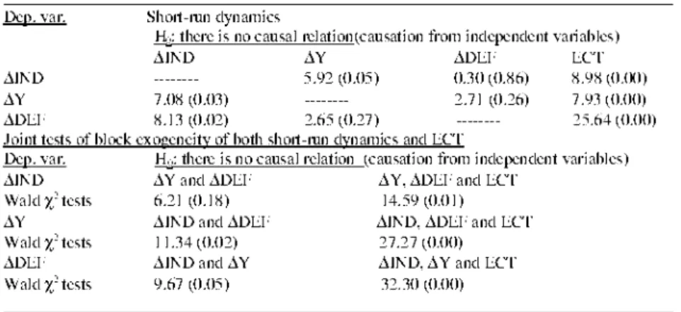
Table 7. Granger Causality Analysis For Model III Dep. var. Short-ran dynamics
H j there is no causal ¡elation(causation from independent variables) A I M ) AY ADEE E C T AI K D 5 . 9 2 ( 0 . 0 5 ) 0 . 3 0 ( 0 . 8 6 ) 8 . 9 8 ( 0 . 0 0 ) AY 7.08 (0.03) 2 . 7 1 ( 0 . 2 6 ) 7.93 (0.00)
A D E f 8.13 (0.02) 2.65 (0.27) 2 5 . 6 4 ( 0 . 0 0 ) Joint tests of block exogeneity of both short-ran dynamics and E C T
Dep. var. I-E: there is no causal relation [causation from independent variables) AI K D AY and ADEE AY, ADEE and E C T
Wald tests 6 . 2 1 ( 0 . 1 8 ) 14.59(0.01) AY A I N D and ADEE A1ND, ADEE and E C T
Wald y; tests 1 1.34 (0.02) 27.27 (0.00) ADEI • A I N D and AY AIND, AY and E C T Wald y; tests 9.67 (0.05) 32.30 (0.00)
From Tab. 5 to Tab. 7, wc examine causal relationships derived Irom Granger causality tests assuming both exogeneity of each variables with lagged dynamic structure and block exogeneity of all the variables under the null hypothesis in each equations. In the upper part of the tables, we examine separately statistical significance of the sum of the lags of each explanatory variables as well as the significance of one-period lagged error-correction term (ECT) taken Irom the long-tem co-integrating relationship, while lower part of
the tables is devoted ID testing LIOIH the block exogeneity of all ihe differenced
explanatory variables and those plus the signilicance of lagged error-correction term as a whole, which, for the latter case, tests the strong exogeneity of dependent variable under the null hypothesis. The test statistics in the tables are yielded by the Wald %2 tests distributed with d.o.f. the number of restrictions. The numbers in paranthesis are probability (Prob.) values of relevant statistics, for which we accept that Prob. values lower than 0.05 would indicate the rejection of the null hypothesis in favor of the statistical signilicance of the restrictions applied for causality tests.
In Tab. 5. we lind that short-run causality runs from total energy consumption to the changes in the general price deflator, and such a case is supported by the fact that the only significant error correction coefficient is that of the changes in price dell at or, i.e., that of the domestic inllation. This reveals also the endogenous characteristic of general price level as for the total energy consumption so that we can easily assume that shocks on energy prices are directly transmitted into the changes in general price level when we consider the short-run causal relations between the variables of interest. These results are strongly verilied by the rejection of the strong exogeneity for the only domestic inllation data in the lower part of the Tab. 5. Therefore, the lack of evidence in favor of the causal relationship between changes in total energy consumption and real income growth gives support to the neutrality hypothesis explained above. Besides, the estimation results for the causal relationships between changes in total energy consumption, real income growth and domestic inllation are nearly same as the causal relations between the changes in residential and commercial energy consumption, real income growth and domestic inllation data used in Tab. 6 except the finding that strong exogeneity of the changes in residential and commercial energy consumption has now been rejected in the lower part of the Tab. 6. As for the short-run dynamics, though there seems to be a signilicant shon-run Granger causality running
Evidence I r o m Turkey
from real income growth rale 10 changes in residential and commercial energy consumption data lor the Model 2. the insignificance of the error-correction term precludes any long-run knowledge of causal relationship. Thus, the causality in the system of variables is carried out in general by affecting the domestic inllationary Iramework of the economy. In a different sense, these results emphasize that for the Model 1 and Model 2 changes in energy consumption and real income should be considered exogenous to the course of domestic inllation at least when we consider the shon-run dynamics.
In Tab. 1 above, we can easily notice that the predominant component of the energy consumption data in the Turkish economy is to a greater extent that of the industrial consumption. In Tab. 7 assuming industrial consumption as the relevant energy consumption data, all the error-correction coefficients have statistical significance, while there seems to be a short-run mutual causal relationship between real income growth and changes in industrial consumption. We also find that the strong exogeneity of all variables can now be rejected when the causal effects of error-correction terms are taken into account by the Wald test statistics, which leads us to extract the knowledge of that all the variables tend to be in this case in a long-run as well as in a short run causal relation by imposing each other an endogenous characteristic.
Following these estimation lindings, we can conclude that the Turkish data requires for the causality issues between changes in energy consumption, real income growth and domestic inflation that we need to make a distinction between different groups of energy consumption data considered in these relations. There exists a mutual relationship in both short and long- run between all the variables in so far as the industrial consumption data is used for relevant energy consumption data, and following this finding is that the neutrality hypothesis between changes in energy consumption and real income growth in addition to the domestic inflation variable used in this paper can be rejected provided that industrial energy consumption data are of special
c one cm lor the empirical purposes. Bui when the loial energy consumption or residential and commercial enery consumption data are considered, the main causal relations and the feedback effects leading us to the existence ol a steady-state relationship run Iroin changes in energy consumption and real income to the changes in general price level. Thus the main policy conclusion extracted from the analysis implemented thus far can be summarized such that energy policies ex-artte designed have the power of affecting the domestic in nation in a predominant way in the economy, for we find that the main endogenous factor upon which other factors in the causal system, i.e.. real income growth and changes in energy consumption, have the tendency to lead to the causal effects is the changes in the price level, i.e.. domestic inllation.
7. CONCLUDING REMARKS
The potential links between energy consumption and real income have been of special importance in designing discretionary macroeconomic policies for stabilization purposes, and impact of this relation upon the issue of how changes in energy consumption and the course real income growth affect the purpose of price stability needs to be examined elaborately for developed as well as developing countries. Thus revealing the direction of causal relations between these macroeconomic aggregates give economic agents and policy makers significant knowledge in policy design and implementation process so as to assess the long-run course of the energy policies.
In our paper, we try to examine the long- and the short-run causal relations between change in energy consumption, represented by electric power consumption, real income growth and domestic inllation in the Turkish economy. Based on a contemporaneous multivariate co-integrating framework, our estimation results indicate that a distinction between various categories of energy consumption needs to be made when the causality issues are to be highlighted. For this purpose, we construct three distinctive models as for the energy consumption data considered, i.e.. total energy consumption, residential
Evidence I r o m Turkey
and commercial energy consumption and industrial energy consumption. We lind that the so-called neutrality hypothesis that means no causal relations found between change in energy consumption and economic growth cannot be rejected for the model using total energy consumption data. For the model using residential and commercial enery consumption data we have some conflicting results for the long- and the short-run dynamics, but can express briefly that there seems to be a causal link towards the changes in energy consumption through the real income growth. But the vital point to be emphasized can be generalized such that domestic inflationary Iramework is found highly endogenous to all the model constructions and thus subject to the changes in especially energy consumption data in addition to the real income growth. Besides, both short- and long-run causal relations verify these findings. For the special case of Model 3 using industrial consumption as the relevant energy consumption data, there seems to be a long-run causal relationship between all the variables, for they have highly endogenous characteristics against each other within the causality analysis. Thus, we reject the neutrality hypothesis for this model.
All in all, we conclude that energy policies ex-ante designed have the power of affecting the domestic inflation in a predominant way and for the case of industrial energy consumption data energy conservation policies may lead to harmful results for the real income growth process though the latter issue is not the relevant case for residential and commercial energy consumption and total energy consumption data.
REFERENCES
1. AKARCA, A T. and LONG, T.V. (1980), "On the Relationship between Energy and GNP: A Reexamination", Journal of Energy and Development, 5, 326-33}.
2. AL-IRIANI, M. (2006), "Energy-GDP Relationship Revisited: An Example from GCC Countries Using Panel Causality", Energy Polity, 34, 3342-3350. 3. ANDERSON, R. G., HOFFMAN, D. and RASCHE, R. H. (1998), ",4 Vector Error Correction Forecasting Model of the U.S. economy", The Federal Reserve Bank of St Louis Working Paper, 98-008A, May.
4. ASAFU-ADJAYE, J. (2000), "The Relationship between Energy Consumption, Energy Prices and Economic Growth: Time Series Evidence from Asian Developing Countries", Energy Economics, 22, 615-625.
5. DICKEY, D.A. and FULLER, W.A. (1979), "Distribution of the Estimators for Autoregressive Time Series uith a Unit Root", Journal of the American Statistical Association, 74, 427-431.
6. DICKEY, D.A. and FULLER, W.A. (1981), "Likelihood Ratio Statistics for Autoregressive Time Series with Unit Roots", Econometrica, 49, July,
1057-1072.
7. DICKEY, D. A., JANSEN, D. W. and THORNTON, D. L. (1991), ".4 Primer on Cointegration uith an Application to Money and Income", The Federal Reserve Bank of St. Louis Review, March/April, 58-78.
X. DOORNIK, J.A., HENDRY, D.F. and NIELSEN, B. (1998), "Inference in Cointegrating Models: UK Ml Revisited", Journal of Economic Surveys, 12/5,
533-572.
9. ELLIOTT, G„ ROTHENBERG, T.J. and STOCK, J.H. (1996), "Efficient Tests for an Autoregressive Unit Root" , Econometrica, 64, 813-836.
10. ENDERS, W. (2004), Applied Econometric Time Series, John Wiley &
Sons, Inc.
Evidence I r o m Turkey
11. ENGLE, R. F. and GRANGER. C. W. J. (1987), "Co-integration and Error Correction: Representation, Estimation, and Testing", Econometrica, 55, 251-276.
12. EROL, U and YU, E.S.H. (¡987), "On the Causal Relationship between
Energy and Income for Industrialized Countries", Journal of Energy and Development, 13, 113-122.
13. GHAU, K.H. and EL-SAKKA, M.I.T. (2004), "Energy Use and Output
Growth in Canada: A Multivariate Cointeg ration Analysis", Energy Economics, 26, 225-238.
14. GLASURE, YONG U. and LEE, Aie-Rie (1997), "Cointegration,
Error-correction, and the Relationship between GDP and Energy: The Case of South Korea and Singapore ", Resource and Energy Economics, 20, 17-25.
15. GONZALO, J. (1994), "Five Alternative Methods of Estimating Long-run Equilibrium Relationships ", Journal of Econometrics, 60, 203-233.
16. GRANGER, C.W.J. (1969), "Investing Causal Relations by Econometric
Models and Cross Spectra! Methods", Econometrica, 37, 424-438.
17. GRANGER, C. W. J. (1986), "Developments in the Study of Cointeg rated
Economic Variables", Oxford Bulletin of Economics and Statistics, 48/3, 213-228.
IS. GRANGER, C.W.J. (1988), "Some Recent Developments in a Concept of
Causality", Journal of Econometrics, 39, 199-211.
19. GRANGER, C.W.J, and NEWBOLD, P. (1974), "Spurious Regressions in
Economics, Journal of Econometrics, 2/2, 111-120.
20. HARRIS, R.I.D. (1995), Using Cointegration Analysis in Econometric Modelling, Prentice Hall.
21. HENDRY, D. F. (1986), "Econometric Modelling with Cointegrated Variables: An CX'ei~view", Oxford Bulletin of Economics and Statistics, 48/3, 201-212.
22. HONDROYIANNIS. G„ LOWS. S. and PAPAPETROU. E. (2 002). "Energy Consumption and Economic Growth: Assessing the Evidence from Greece", Energy Economics, 24, 319-336.
23. HWANG, D.B.K. and GUM, B. (1992), "The Causal Relationship between Energy and GNP: The Case of Taiwan", Journal of Energy and Development, 16, 219- 226.
24. JOHANSEN, S. (1988), "Statistical Analysis of Cointegration Vectors",
Journal of Economic Dynamics and Control, 12, 231-254.
25. JOHANSEN, S. (1992), "Determination of Cointegration Rank in the
Presence of a Linear Trend", Oxford Bulletin of Economics and Statistics, 54/3, 383-397.
26. JOHANSEN, S. (1995). Likelihood-based Inference in Cointegrated
Vector Autoregressive Models, Oxford University Press.
27. JOHANSEN, S. and JUSELIUS, K. (1990), "Maximum Likelihood Estimation and Inference on Cointegration-with Applications to the Demand for Money", Oxford Bulletin of Economics and Statistics, 52, 169-210.
28. JOHANSEN, S. and JUSELIUS, K. (1992), "Testing Structural Hypotheses in a Multivariate Cointegration Analysis of the PPP and the UIP for UK", Journal of Econometrics, 53, 211-244.
29. JUMBE, C.B.L, (2004), "Electricity Consumption and GDP: Empirical
Evidence from Malawi", Energy Economics, 26, 61-68.
30. KRAFT, J. and KRAFT, .4. (1978), "On the Relationship between Energy
and GNP", Journal of Energy and Development, 3, 401-403.
31. LEE, C.-C. (2005), "Energy Consumption and GDP in Developing Countries: .4 Cointegrated Panel Analysis", Energy Economics, 27, 415-127. 32. MACKINNON, J.G. (1991), "Critical Values for Cointegration Tests", Long-run Economic Relationships: Readings in Cointegration, Ch. 13 (Eds. R. F. Engle and C. W. J. Granger) , Oxford: Oxford University Press.
Evidence I r o m Turkey
33. MACKINNON, J.G. (1996), "Numerical Distribution Functions for Unit Root and Coin! eg ration Tests", Journal of Applied Econometrics, 11, 601-618.
34. MAHADEVA, L. and ROBINSON. P. (2004), "Unit Root Testing to Help Model
Building", Handbooks in Central Banking, (Eds. Andrew Blake and Gill Hammond), Centre for Central Banking Studies, Bank of England, No. 22, July.
35. MASIH, A.M.M. and MASIH, R. (1996), "Energy Consumption, Real Income and Temporal Causality: Results from a Multi-country Study Based on Cointegration and Error-correction Modelling Techniques", Energy Economics, 18, 165-183.
36. MASIH, A.M.M. and MASIH, R. (1997), "On the Temporal Causal Relationship between Energy Consumption, Real Income, and Prices: Some New Evidence from Asian-Energy Dependent NICs Based on a Multivariate CointegrationA7ector Error Correction Approach", Journal of Policy
Modeling, 19/4, 417-440.
37. MASIH, A.M.M. and MASIH, R. (1998), "A Multivariate Cointegrated Modelling Approach in Testing Temporal Causality between Energy Consumption, Real Income and Prices with an Application to Two Asian LDCs", Applied Economics, 30, 1287-1298.
3<S. MEHRARA, M. (2007), "Energy Consumption and Economic Growth: The
Case of Oil Exporting Countries", Energy Policy, 35, 2939-2945.
39. NELSON, C. and PLOSSER, C. (1982), "Trend and Random Walks in Macroeconomic Time Series: Some Evidence and Implications", Journal of Monetary Economics, 10, 130-162.
40. OH, W. and LEE, K. (2004), ''Energy Consumption and Economic Growth
in Korea: Testing the Causality Relation", Journal of Polity Modeling, 26, 973-981.
41. Prime Ministry Republic of Turkey Turkish Statistical Institute (2006),
Statistical Indicators 1923-2005, December.
42. QMS (2004), EViews 5 User's Guide. April.
43. SIMS, C. (1972), "Money, Income and Causality", A men can Economic Review, 62, 540-552.
44. SOTTAS, U. and SARI, R. (2003), "Energy Consumption and GDP: Causality Relationship in G-7 Countries and Emerging Markets", Energy Economics, 25, 33- 37.
45. YU, E.S.H. and JIN, B.K. (1984), "The Relationship between Energy and GNP: Further Results", Energy Economics, 6, 168-190.
46. YU, E.S.H. and CHOI, J.Y. (1985), "The Causal Relationship between
Energy and GNP: An International Comparison", Journal of Energy and Development, 10, 249-272.
47. YU, ES.H. and JIN, J.C. (1992), "Cointegration Tests of Energy Consumption, Income and Employment", Resources and Energy, 14, 259-266. 4H. YULE, G. (1926), "Why do We Sometimes Get Nonsense Correlations between Time Series? .4 Study in Sampling and the Nature of Time Series", Journal of Royal Statistical Society, 89, 1-64.