THE CONDITIONAL EFFECTS
OF EXTERNAL DEBT ON INFLATION
Mustafa Uğur KARAKAPLAN*
Abstract
Although the literature on the determinants of inflation is voluminous, no particular at-tention has been paid to the role of external debt as a specific component of the government debt stock. Also the question of whether and how the effect of external debt on inflation varies with financial market development needs an empirical investigation. Using an unbalan-ced panel data and GMM estimation method, this paper aims to fill this gap by testing two main hypotheses: The first is that the external debt is less inflationary when financial markets are well developed. The second is that the effects of the determinants of inflation are hetero-geneous across countries in extent and in sign. This paper presents robust empirical support for these hypotheses.
Key terms: External Debt, Inflation JEL classification codes: E31, H63
Özet
Enflasyonun etkenleri hakkındaki literatürün oldukça geniş olmasına rağmen devletin borç stokunun belirli bir unsuru olan dış borcun etken rolüne literatürde pek değinilmemiştir. Ayrıca finansal piyasalardaki kalkınmanın dış borcun enflasyon üzerindeki etkisini ne derece etkilediği de araştırılması gereken bir konudur. Bu makale dengelenmemiş panel veri ve GMM metodu kullanarak iki hipotezi test etmektedir: Finansal piyasaları daha gelişmiş ülke-lerde dış borç enflasyona daha az sebep olur; enflasyonun etkenlerinin işaretleri ve dereceleri ülkelere göre değişkendir. Bu makale bu hipotezleri güçlü bir şekilde desteklemektedir.
Anahtar terimler: Dış borç, Enflasyon JEL sınıflandırma kodları: E31, H63
Introduction
Sargent and Wallace (1981: 6-7) show that in an economy where go-vernment taxes and spending are exogenous, bond-financed deficits are not
sustainable, and the central bank is ultimately forced to monetize the deficit. In the long run, the consequential increase in the money supply is inflatio-nary. Associated with this seminal idea, there has been a growing literature, which aims to identify the impact of fiscal policy on inflation in developed and developing countries. More specifically, the empirical relationship between the deficit and inflation in developed countries has been studied by King and Plosser (1985: 147-149), Ho (1988: 34-36) and Burdekin and Wo-har (1990: 50-53). Empirical studies on developing countries include those of Choudhary and Parai (1991: 1117), Dogas (1992: 367), Sowa (1994: 1105-1106), and Metin (1995: 513-514).
Metin (1998: 412-413) uses a multivariate co-integration analysis to examine the relationship between budget deficit and inflation in Turkey and finds that inflation in Turkey is significantly affected by budget deficits. Another line of research deals with the relationship between sovereign debt and inflation. Kenc et al. (2001: 366-367) is a theoretical study of the relati-onship between inflation and sovereign insolvency. They use a continuous-time model of government budget constraint, and present that it is not the nominal or domestic currency debt but the total debt which generates infla-tion. The authors explain that higher indexed debt or foreign debt should have the same outcome on inflation as the nominal debt due to crowding out of the resources that could have been allocated to help nominal debt.
The idea that financial market development may play an essential role in how monetary and fiscal policies affect inflationary pressures has some empirical support in the literature. For example, Liu and Adedeji (2001: 41-43) study the determinants of inflation in the Islamic Republic of Iran using a structure where they assume an underdeveloped financial market for the country with limited financial assets, functioning under an administratively controlled interest rate. They present evidence that inflation is a monetary phenomenon in Iran. Neyapti (2003: 458-461) uses a panel data set including developed and less developed countries, and finds that the independence of the central bank and financial market development is effectual on the effects of budget deficit on inflation.
When assessing the role of financial market development on inflation rates, one should be cautious about a reverse causality. Huybens and Smith (1999: 283-287) provide evidence that there is a negative correlation between financial market development and inflation. The authors also
pre-sent a threshold effect that the negative relationship between financial mar-ket development and inflation weakens if inflation continues to be above a critical rate. Boyd et al. (2001: 221-226) suggests that the direction of causa-lity goes from inflation to financial activity. They test the theoretical expec-tation that an increase in inflation rates hampers financial market allocation efficiency. They show that higher levels of inflation impede both equity market activity and the banking sector development. They also find thres-hold effects in the relationship that economies with an inflation rate higher than 15 percent are likely to experience discrete reduction in the performan-ce of the financial sector. In a more reperforman-cent study Khan et al. (2006: 165-170) tests the existence of a threshold rate of inflation at which the sign of the effect of inflation on financial deepening is changed. The authors utilize a cross-country sample, and depending on the measures used to proxy finan-cial depth, they find empirical support for the presence of a threshold rate of inflation around 3-6 percent per year. For the purpose of this study, these findings point out to a potential problem of endogeneity that has to be dealt with when assessing the impact of financial market development on the rela-tionship between external debt and inflation.
Akinboade, Niedermeier and Siebrits (2002: 213) analyze the determi-nants of inflation in South Africa using a model where inflation is potentially affected by changes in the money, labor and foreign exchange markets. They find that inflation in South Africa is generally a structural phenomenon whe-re incwhe-reases in unit labor costs and broad money supply awhe-re likely to incwhe-rease inflation. Unlike those studies where the main interest is to study the deter-minants of the rate of inflation, Boschen and Weise (2003: 323-325) look at a slightly different aspect of the factors associated with inflation. They in-vestigate the beginnings of inflationary periods utilizing a pooled data set including 73 inflation episodes in OECD countries since 1960. They find that national elections and high real growth targets are the most important factors in initiating inflation episodes. They also suggest that the inflation in the U.S. generates concurrent outbreaks of inflation in these counties. Anot-her aspect of inflation that varies across countries is volatility. Aisen and Veiga (2008: 207-209) examine the determinants of the inflation volatility using a linear dynamic panel data models and GMM estimation methodo-logy. They find that higher political instability and lack of central bank inde-pendence result in more unstable inflation rates.
Finally, political stability is another factor that is hypothesized to affect inflation. An important study along these lines is Desai, Olofsgard and You-sef (2003: 391-392). They study the effect of political openness and income inequality on inflation. They present robust evidence that democracy is asso-ciated with higher inflation in higher-inequality countries but with lower inflation in lower-inequality countries. Aisen and Veiga (2006: 1379-1382) estimate the relationship between inflation and political instability control-ling for the endogeneity. They propose that higher degrees of political insta-bility cause higher seigniorage and inflation rates. Moreover, it is presented that the system is more pervasive and stronger in developing countries, espe-cially in those with high inflation rates.
The first goal of this study is to shed some light on the role of foreign debt on inflationary pressures and how this role is influenced by the degree of financial market development. With a parallel idea to that in Neyapti (2003: 458-461), which examines the relationship between budget deficits and inflation rates, this paper investigates the specific effect of external debt on inflation, and hypothesizes that the effect is not necessarily positive and is subject to the level of financial market development within the countries. In particular, this paper tests the validity of the idea that if the financial market is well developed, the debt may be less inflationary or even not inflationary at all. The second goal is to check the robustness of the results with respect to differences in main country characteristics. If the relationship between the determinants of inflation and the inflation rates varies across countries, the coefficients of the determinants of inflation would be expected to be diffe-rent in extent and in sign for diffediffe-rent country groups. To test this hypothesis the effects are allowed to vary by whether the country is a Latin American country, a high inflation country, a European Union country or a transition country.
1. Models
Neyapti (2003: 461) formulate money demand as:
where denotes time, is money, is price level, is both interest ra-tes and real income, and is inflationary expectations. is assumed to be
constant and bigger than . Equation presents that there is a negati-ve relationship between real money demand and expected inflation rate. Neyapti (2003: 461) also assumes rational inflationary expectations. By first differencing the continuous forward substitutions for the expectational diffe-rence equation for price level, the following equation can be derived:
where is the operator for differencing such that for every . In this equation the positive relationship between current price level and present value of the expected changes in the money supply is expressed.
Neyapti (2003: 461) presents the budget constraint equation of the go-vernment, and states that the deficits are financed by new debt or issuing money. Subsequently, the relationship between deficit and inflation is asser-ted to be subject to financial market development:
where denotes government expenditures, is revenues from tax, is the nominal interest rate, B is government debt, denotes the lack of financial market development, and is financing requirements of the government. When the expectation of equation is integrated in equation
one gets:
This article analogously formulates the inflation with growth rate of money, growth rate of real output and lagged inflation rates. Furthermore, it is assumed that the budget deficit is financed by external debt. Hence, the effect of external debt is expected to be subject to the development in finan-cial markets. Considering the extreme cases, if the finanfinan-cial markets are fully developed the degree of monetary accommodation of external debt is equal to zero, which in turn states that external debt is not inflationary at all. Conversely, if there is a perfect lack of financial market development monetary expansion satisfies all of the financing of the budget constraint, that is, external debt results in inflation.
Hence, the first hypothesis of this paper is that the external debt is less inflationary where financial markets are well developed. In order to control this hypothesis, interactive terms of external debt with financial market de-velopment (FMD) indicators are added to the basic model. Equation presents the basic model:
The model predicts the effect of lagged inflation and growth of money on inflation to be positive, and the effect of growth of real output on inflation to be negative. External debt is expected to be inflationary, but less inflatio-nary in more developed financial markets.
Moreover, the effects of all variables are controlled for heterogeneity across countries. Latin American countries (LA), European Union (EU) co-untries, high inflation1 countries (HI) and transition countries2 (TR) are gro-uped, and the effects of all variables are checked for country groups in sepa-rate models. The second hypothesis is that the effects of variables on infla-tion are heterogeneous across countries, which means that the regression results of the basic model cannot be generalized. Country group (CG) mo-dels are represented by equation (6):
2. Data
This study uses a panel data set obtained from two sources: Main eco-nomic indicators are obtained from World Development Indicators (WDI) Online and IMF international financial statistics (IFS). Due to the
1 Annual inflation that is bigger that %50 is assumed to be high. A country with a high inflation
period is thus assumed to be a high inflation country.
lity from these sources, the data set covers only the period of 1960−2004 and it is composed of 121 countries. Since there are some missing observations for some variables in different time periods for different countries, the data is unbalanced.
The main variables employed in the basic model consist of inflation, external debt, growth of gross domestic product (GDP) and growth of mo-ney. Annual inflation in consumer prices (inf) is converted to D, which is the loss in the real value of money as in Cukierman et al. (1992: 370)3, and is
used as the endogenous variable. Share of external debt in GDP (sEDebt) is taken as the debt measure. Moreover, in order to control the effects of past inflation on current inflation, the first lag of D (D (−1)) is inserted as an explanatory variable. Growth in GDP (gGDP) and growth in money (gM) are added to models to control for the effects of growth of GDP and growth of money on inflation.
In addition to all these control variables, there are interaction terms of sEDebt with FMD indicators. This study uses three FMD indicators. These indicators report to what extent the financial market is developed and higher values mean better financial market conditions. FMD indicators are normali-zed between 0 and 1. These indicators are share of money and quasi money in GDP (sM2); share of total claims of deposit money banks in GDP (sCR); and share of claims of deposit money banks on private sector in GDP (sCRpr). FMD interaction terms appearing in the models are the product of sEDebt with FMD indicators (sEDebt × FMD). Moreover there are four CG which are LA, EU, HI and TR which are interacted with all variables to check the effects for country groups in separate models.
3. Methodology
The general static single-equation panel model is:
where is a vector of explanatory variables, is the time specific effect, is the country specific effect, is the error term, is the time ran-ge and is the number of countries. When explanatory variables include
some of the lagged values of dependent variables, the model becomes dyna-mic. A dynamic model can be written as:
where lagged values of dependent variables are available, is a vector of K explanatory variables, is the country specific effect, is the error term, is the number of time periods for country , and is the number of countries.
Nickell (1981: 1425) explains that the dynamic character of the model and existence of individual specific fixed effects result in inconsistent esti-mates in OLS estimation of the models, and the asymptotic biases are shown to be large and matching with the estimates in Nervole (1967: 42) and Mad-dala (1971: 341). Since the models in this study have explanatory variables including some lagged values of the dependent variable and the panel data set is unbalanced; dynamic panel data estimation method developed by Arel-lano and Bond (1988: 5) is found to be the appropriate econometric tech-nique to estimate the models4. Doornik, Arellano and Bond (2002) is utilized
to apply the unbalanced panel data set in a proper way, and to use the gene-ralized methods of moments (GMM).
In order to remove country specific fixed effect biases, the estimations take the first differences of all variables in the equation. This transformation causes a decrease in the number of observations by the number of cross-section observations, and in turn a loss in degrees of freedom in estimation. Although, the basic model assumed to have white-noise errors; the transfor-mation causes first order serial correlation in the error terms. Hence, instru-mental variables technique is employed to avoid this serial correlation. In all regressions, the set of instrument variables is composed of first lag of all explanatory variables except D (−1). The first and second moments of the rest of the lags of the dependent variable that is not used in the explanatory part of the model, is built with GMM technique in Arellano and Bond (1988: 5) and applied as the GMM instrument.
4 In order to verify the dynamic nature of the model, individual effects are controlled. Since the
hypothesis on dummies including individuals is rejected with Wald test statistic, the model is found to be valid for a dynamic study.
The Sargan test is used to test the validity of instrumental variables. The hypothesis being tested is that the instrumental variables are uncorrela-ted with a set of residuals, and hence instruments are suitable. If the null hypothesis is not rejected by the statistic, the instrumental variables are valid to be used.
AR (m) tests are used to test the existence of mth order serial
correla-tion. The hypothesis being tested is that there does not exist mth order serial
correlation. If the null hypothesis is rejected, there exists mth order serial
correlation. Since dynamic panel data involves an AR (1) process for the error terms, the lack of second order autocorrelation is the main concern, which thus requires the non-rejection of H0 = no AR (2) or H0 = no m2 as in
Arellano and Bond (1991: 288-293).
Moreover, Wald tests are used to test the significance of groups of vari-ables. Wald (Joint) test in the tables are on all explanatory variables except dummies. The null hypothesis being tested with Wald (Joint) test is that none of the coefficients, excluding the constant, in the model is statistically signi-ficant. If the null hypothesis is rejected by the statistic, then at least one of the coefficients is statistically significant. Wald (Dummy), Wald (terms) tests are similar tests to check the significance of dummies including cons-tant term, and significance of all specified terms respectively.
4. Estimation Results
In all models, Sargan test results report that instrumental variables are found to be uncorrelated with the error terms, m2 tests present that there is no
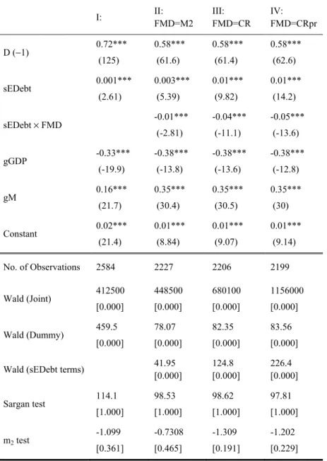
second order serial correlation, and Wald test results indicate that at least one of the coefficients is significantly different than zero. Table 1 reports the regression results of basic model. In the first column of Table 1, no interac-tion terms of sEDebt is inserted. As being expected, coefficients of D (−1), sEDebt and gM are found to be positive and significant at 1% level and hig-her GDP growth is found to lower inflation.
In the second, third and fourth column of Table 1, interaction terms of sEDebt with sM2, sCR and sCRpr are integrated respectively. Supporting the first hypothesis, interactive terms of sEDebt are found to have a signifi-cant and negative effect on D, which means that when the financial markets are well developed, external debt is less inflationary. Effects of other variab-les are significant and similar to results in the first column.
Table 1: Regression results of the basic model Dependent Variable: D I: II: FMD=M2 III: FMD=CR IV: FMD=CRpr D (−1) 0.72*** (125) 0.58*** (61.6) 0.58*** (61.4) 0.58*** (62.6) sEDebt 0.001*** (2.61) 0.003*** (5.39) 0.01*** (9.82) 0.01*** (14.2) sEDebt × FMD -0.01*** (-2.81) -0.04*** (-11.1) -0.05*** (-13.6) gGDP -0.33*** (-19.9) -0.38*** (-13.8) -0.38*** (-13.6) -0.38*** (-12.8) gM 0.16*** (21.7) 0.35*** (30.4) 0.35*** (30.5) 0.35*** (30) Constant 0.02*** (21.4) 0.01*** (8.84) 0.01*** (9.07) 0.01*** (9.14) No. of Observations 2584 2227 2206 2199 Wald (Joint) 412500 [0.000] 448500 [0.000] 680100 [0.000] 1156000 [0.000] Wald (Dummy) 459.5 [0.000] 78.07 [0.000] 82.35 [0.000] 83.56 [0.000]
Wald (sEDebt terms) 41.95
[0.000] 124.8 [0.000] 226.4 [0.000] Sargan test 114.1 [1.000] 98.53 [1.000] 98.62 [1.000] 97.81 [1.000] m2 test -1.099 [0.361] -0.7308 [0.465] -1.309 [0.191] -1.202 [0.229] Notes: Numbers in parentheses are the t-ratios; numbers in brackets are the p-values. *** indicates significance at 1% level.
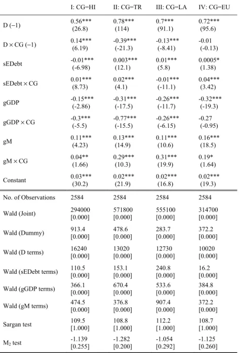
In Table 2, regression results from country group models are reported. Most of the coefficients in Table 2 are found to be statistically significant. However the effects of some of variables are found to be different than that of initial variables in magnitude and in sign which supports the second hy-pothesis.
In all country groups effect of D (−1) is found to be positive as in Table 1. Nevertheless, the interaction term of D (−1) with TR and LA are found to be negative and significant, which means that although previous inflation is positively effectual on current inflation, if the country is a transition or a Latin American country, the effect may be smaller.
Interestingly, for high inflation countries the effect of sEDebt is found to be negative where coefficient of interaction term of sEDebt with HI is positive, which suggests that if the country is a high inflation country, exter-nal debt is positively effectual on inflation whereas it is negatively effective in general. For LA group, the results are the opposite that is the effect of sEDebt is positive whereas the effect of interaction term of sEDebt with LA is negative. This indicates that external debt is not necessarily positively effectual on inflation. If the country is a Latin American country, the effect may be negative.
For the other coefficients the results are not different in sign from Table 1. gGDP is found to be negatively effectual on inflation regardless of co-untry group. Coeffecient of gM is found to be significant and positive in all columns which are similar to results in Table 1. However, these coefficients are different in extent for country groups which should be taken into acco-unt.
Table 2: Regression results of the CG model Dependent Variable: D
I: CG=HI II: CG=TR III: CG=LA IV: CG=EU
D (−1) 0.56*** (26.8) 0.78*** (114) 0.7*** (91.1) 0.72*** (95.6) D × CG (−1) 0.14*** (6.19) -0.39*** (-21.3) -0.13*** (-8.41) -0.01 (-0.13) sEDebt -0.01*** (-6.98) 0.003*** (12.1) 0.01*** (5.8) 0.0005* (1.38) sEDebt × CG 0.01*** (8.73) 0.02*** (4.1) -0.01*** (-11.1) 0.04*** (3.42) gGDP -0.15*** (-2.86) -0.31*** (-17.5) -0.26*** (-11.7) -0.32*** (-19.3) gGDP × CG -0.3*** (-5.5) -0.77*** (-15.5) -0.26*** (-6.15) -0.27 (-0.95) gM 0.11*** (4.23) 0.13*** (14.9) 0.11*** (10.6) 0.16*** (18.5) gM × CG 0.04** (1.66) 0.29*** (10.3) 0.31*** (19.9) 0.19* (1.64) Constant 0.03*** (30.2) 0.02*** (21.9) 0.02*** (16.8) 0.02*** (19.3) No. of Observations 2584 2584 2584 2584 Wald (Joint) 294000 [0.000] 571800 [0.000] 555100 [0.000] 314700 [0.000] Wald (Dummy) 913.4 [0.000] 478.6 [0.000] 283.7 [0.000] 372.2 [0.000] Wald (D terms) 16240 [0.000] 13020 [0.000] 12730 [0.000] 10020 [0.000]
Wald (sEDebt terms) 110.5 [0.000] 153.1 [0.000] 240.8 [0.000] 16.2 [0.000]
Wald (gGDP terms) 366.1 [0.000] 670.4 [0.000] 533.6 [0.000] 384.8 [0.000]
Wald (gM terms) 474.5 [0.000] 376.8 [0.000] 907.4 [0.000] 372.2 [0.000]
Sargan test 109.5 [1.000] 108.8 [1.000] 112.2 [1.000] 108.7 [1.000]
M2 test -1.139 [0.255] -1.282 [0.200] -1.054 [0.292] -1.125 [0.260]
Notes: Numbers in parentheses are the t-ratios; numbers in brackets are the p-values. *** indicates significance at 1% level. ** indicates significance at 5% level. * indicates significance at 10% level.
Conclusion
Two hypotheses are tested in this paper: The first hypothesis is that the external debt is less inflationary if financial markets are well developed; the second hypothesis is that the effects of the determinants of inflation are hete-rogeneous across countries in extent and in sign. An unbalanced panel data set including 121 countries and the period of 1960−2004, where available, is used in the empirical analysis. The analysis accounts for changes in the level of FMD, and LA, HI, EU and TR country groups explicitly. Since the model includes first lag of inflation and data set is unbalanced, in order to prevent estimation problems, GMM technique is utilized.
When the effects of determinants are assumed to be homogenous across countries, the results support the first hypothesis proposing that the debt is less inflationary in economies with well developed financial markets. Hence, the findings in the literature are subject to the development level of the fi-nancial sectors of the countries. Also, the results present that the coefficients of variables differ in country groups, which support the second hypothesis suggesting that the relationships are heterogeneous across countries. There-fore contrary to the suggestions in the literature, the effects of determinants on inflation cannot be assumed to be homogeneous, that is, the results in the homogeneous model cannot be generalized.
References
Aisen, A; Veiga, F. J. (2006). “Does Political Instability lead to higher inflation? A Panel Data Analysis”. Journal of Money, Credit, and Banking, 38, (5), 1379-1389.
Aisen, A. and Veiga, F. J. (2008), “Political instability and inflation volatility” Public Choice, 135, 207–223.
Akinboade, O.A; Niedermeier, E.W; Siebrits, F.K. (2002). “The Dynamics of Inflation in South Africa: Implications for Policy”. South African Journal of Economics, 70 (3): 213-223.
Arellano, M; Bond, S. (1988). “Dynamic Panel Data Estimation Using DPD”. Institute of Fiscal Studies. Working Paper Series no: 88/15..
Arellano, M; Bond, S. (1991). “Some Tests of Specification for Panel Data: Monte Carlo Evidence and an Application to Employment Equations”. The Review of Economic Studies. 58 (2): 277-297.
Boschen J. F. and Weise C. L. (2003), “What Starts Inflation: Evidence from the OECD Countries”, Journal of Money, Credit and Banking, 35 (3), 323-349.
Boyd, J. H., R. Levine and B. D. Smith (2001), “The impact of inflation on financial sector performance”, Journal of Monetary Economics 47, 221-248.
Burdekin, R. C. K., and Wohar, E. M. (1990)," Deficit Monetisation, Output and Inflation in the United States, 1923-1982," Journal of Economic Studies, 17, 50-63.
Choudhary, M. A. S., and Parai, A . K. (1991)," Budget Deficit and Inflation: The Peruvian Experience," Applied Economics, 23, 1117-1121.
Cukierman, A., Webb, S., Neyapti, B, (1992). “Measuring the Independence of Central Banks and Its Effect on Policy Outcomes”. World Bank Economic Review, 6: 353–98. Desai, R. M; Olofsgard, A; Yousef T. M. (2003), “Democracy, Inequality, and Inflation”,
American Political Science Review, 97 (3), 391-406.
Dogas, D. (1992)," Market Power in a Non-monetarist Inflation Model for Greece," Applied Economics, 24, 367-378.
Doornik, J. A; Arellano, M; Bond, S. (2002). “Panel Data estimation using DPD for Ox”. http: //www.doornik.com.
Ho, L. S. (1988),"Government Deficit Financing and Stabilisation,"Journal of Economic Studies, 15, 34-44.
Huybens E., B. D. Smith (1999), “Inflation, Financial markets and long-run real activity”, Journal of Monetary Economics 43, 283-315.
Kenc, T., W. Perraudin and P. Vitale (2001), “Inflation and Sovereign Default”, IMF Staff Papers, 47 (3), 366-386.
Khan, M.S., A. S. Senhadji,, B. D. Smith (2006), “Inflation and Financial Depth”, Macroeconomic Dynamics, 10, 165–182.
King, R. G., and Plosser, C. I. (1985), "Money Deficits and Inflation," in Understanding Monetary Regimes (Carnegie-Rochester Conference Series on Public Policy, 22), pp. 147-196. Liu, O., Adedeji, O. S. (2001), “Determinants of Inflation In The Islamic Republic of Iran - A
Macroeconomic Analysis”, Macroeconomic Issues and Policies in the Middle East and North Africa. International Monetary Fund, 2001.
Maddala, G. S. (1971). “The Use of Variance Components Models in Pooling Cross Section and Time Series Data”. Econometrica. 39: 341-358.
Metin, K. (1995), "An Integrated Analysis of Turkish Inflation," Oxford Bulletin of Econo-mics and Statistics, 57, 513-533.
Metin, K. (1998), “The Relationship between Inflation and the Budget Deficit in Turkey,” Journal of Business and Economics Statistics, 16 (4), 412-422.
Nervole, M. (1967). “Experimental Evidence on the Estimation of Dynamic Economic Relati-ons from a Time Series of Cross-SectiRelati-ons”. Economic Studies Quarterly. 18: 42-74. Neyapti, B. (2003). “Budget Deficits and Inflation”. Contemporary Economic Policy. 21 (4):
458-475.
Nickell, S. (1981). “Biases in Dynamic Models with Fixed Effects”. Econometrica. 49: 1417-1426. Sargent, T. J., and Wallace, N. (1981), "Some Unpleasant Monetarist Arithmetic," Quarterly
Review, Federal Reserve Bank of Minneapolis, 5, 1-18.
Sowa, N. K. (1994)," Fiscal Deficits, Output Growth and Inflation Targets in Ghana," World Development, 22, 1105-1117.
APPENDIX A1: Country groups
LA countries:Argentina, Bolivia, Brazil, Chile, Colombia, Costa Rica, Cuba, Domi-nican Republic, Ecuador, El Salvador, Guatemala, Haiti, Honduras, Mexico, Nicaragua, Panama, Paraguay, Peru, Uruguay, Venezuela.
HI countries:
Albania, Angola, Argentina, Armenia, Azerbaijan, Belarus, Bolivia, Brazil, Bulgaria, Chile, Democratic Republic of Congo, Costa Rica, Croatia, Dominican Republic, Ecuador, Estonia, The Gambia, Georgia, Ghana, Gui-nea-Bissau, Iceland, Indonesia, Israel, Jamaica, Kazakhstan, Lao PDR, Lat-via, Lithuania, FYR Macedonia, Malawi, Mexico, Mongolia, Mozambique, Myanmar, Nicaragua, Nigeria, Peru, Poland, Romania, Russian Federation, Sierra Leone, Sudan, Suriname, Syrian Arab Republic, Turkey, Uganda, Ukraine, Uruguay, RB Venezuela, Republic of Yemen, Zambia, Zimbabwe.
EU countries:
Austria, Belgium, Cyprus, Czech Republic, Denmark, Estonia, Finland, France, Germany, Greece, Hungary, Ireland, Italy, Latvia, Lithuania, Luxembourg, Malta, The Netherlands, Poland, Portugal, Slovakia, Slovenia, Spain, Sweden, United Kingdom.
TR countries:
Albania, Armenia, Azerbaijan, Belarus, Bosnia and Herzegovina, Bul-garia, Croatia, Czech Republic, Estonia, Georgia, Kazakhstan, Kyrgyz Re-public, Latvia, Lithuania, FYR Macedonia, Moldova, Mongolia, Romania, Russian Federation, Slovak Republic, Slovenia, Tajikistan, Turkmenistan, Ukraine, Uzbekistan.