A test of Black-Litterman portfolio optimization : evidences from bist

(1)

THE REPUBLIC OF TURKEY

BAHCESEHIR UNIVERSITY

A TEST OF BLACK-LITTERMAN PORTFOLIO

OPTIZATION ; EVIDENCES FROM BIST

Master’s Thesis

(2)

(3)

THE REPUBLIC OF TURKEY

BAHÇEŞEHIR UNIVERSITY

GRADUTE SCHOOL OF SOCIAL ACIENCES

CAPITAL MARKETS & FINANCE

A TEST OF BLACK-LITTERMAN PORTFOLIO

OPTIZATION ; EVIDENCES FROM BIST

Master’s Thesis

FARSHAD MIRZAZADEH BARIJOUGH

Supervisor: PROF. DR. MEHMET HASAN EKEN

(4)

THE REPUBLIC OF TURKEY BAHÇEŞEHIR UNIVERSITY

GRADUATE SCHOOL OF SOCIAL SCIENCES CAPITAL MARKETS & FINANCE

Name of the thesis: A TEST OF BLACK-LITTERMAN PORTFOLIO OPTIZATION ; EVIDENCES FROM BIST

Name/Last Name of the Student: Farshad Mirzazadeh Barijough Date of the Defense of Thesis:

The thesis has been approved by the Graduate School of Social Sciences. Yrd. Doc. Burak KUNTAY Graduate School Director

Signature

I certify that this thesis meets all the requirements as a thesis for the degree of Master of Arts.

Doc. Dr. Asli YUKSEL

Program Coordinator Signature

This is to certify that we have read this thesis and we find it fully adequate in scope, quality and content, as a thesis for the degree of Master of Arts.

Examining Comittee Members Signature____

Thesis Supervisor --- Prof. Dr. Mehmet Hasan EKEN

Member ---

Prof. Dr. Umit EROL

Member ---

(5)

ACKNOWLEGMENT

First of all, I would like to express my gratitude to my advisor Prof. Dr. Mehmeh Hasan EKEN, for encouraging and guiding me throughout this study.

Also, I am grateful to my lovely and compassionate parents Najibeh, Ebrahim, and all my precious family, for their endless love and support.

I want to appreciate Financial Research Center of Bahçeşehir University, for providing Bloomberg terminals and other informatics.

Last, I want to thank all of the academic staff working in the Institute of Social Sciences of Bahçeşehir University, who contributed to the synergy around me.

(6)

ABSTRACT

A TEST OF BLACK-LITTERMAN PORTFOLIO OPTIMIZATION; EVIDENCES FROM BIST

Mirzazadeh Barijough Capital Markets And Finance

Thesis Supervisor: Prof. Dr. Mehmet Hasan Eken June 2014, 56 Pages

Harry Markowitz published his Nobel wining article Portfolio Selection in 1952 which is usually seen as genesis of Modern Portfolio Theory. Previous to his works investors were selecting asset portfolios just by their feelings on stock markets return, typically thought of an optimal portfolio as the one who maximized expected return. Markowitz developed a quantitative method to help investment managers to find out optimum weight of assets in portfolio by considering Expected Return and Risk of an investment. This classic Mean-Variance optimal portfolio selection is the foundation of Modern Portfolio Theory. Although Markowitz approach is very popular among investors and fundamentally significant, however since mean-variance optimization in very sensitive to expected returns, and expected returns are very difficult to estimate, the resulting portfolios are unbalanced in most of the cases. It may be the case that an investor wants to impose his or her views depending on a present news. Fisher Black & Robert Litterman were studying on a model to combine historical data and investor’s point of view. Their research published by Goldman Sachs & Company in 1991 as Black-Litterman model.

This study tests these two approaches of asset allocation. First, a detailed description of and CAPM and pitfalls of Mean-Variance model are given. Next we discuss the needs to better model and an overview of Black & Litterman model will be given. Finally, we compare performance of these two models with an empirical test in Istanbul Stock & Exchange (BIST) stocks. Views vector for Black-Litterman model estimated by EGARCH-mean equation in univariate context.

(7)

(8)

Table of Contents Tables ... vii Figures ... viii Abbreviation ... ix Symbols ... x 1.INTRODUCTION ... 1 2. THEORETICAL FRAMEWORK ... 7 2.1 ASSET PROPERTIES ... 7 2.1.1 Classes ... 7

2.1.2 Expected Return And Risk ... 7

2.1.3 Portfolio of Assets ... 9

2.2 THE MARKOWITZ MEAN-VARIANCE OPTIMIZATION ... 11

2.2.1 Model Evolution ... 11

2.2.2 The Mathematics Of The Model ... 14

2.2.3 Drawbacks Of MV Optimization ... 14

2.2.3.1 Utility theory ... 14

2.2.3.2 Normally distributed returns ... 15

2.2.3.3 Deficiencies of mean-variance optimization ... 15

2.2.4 The Separation Theorem ... 16

2.3 CAPITAL ASSET PRICING MODEL ... 18

2.3.1 Assumptions ... 18

2.3.2 Equilibrium ... 18

2.3.3 CAPM Formula ... 19

2.4 THE BLACK-LITTERMAN MODEL ... 20

2.4.1 Model Background ... 21

2.4.2 The Mathematics Of Model ... 23

2.4.2 Expressing The Views ... 26

2.4.2 The Factor Tau ... 29

2.4.3 Following Studies On The Basic Model ... 29

3. LITERATURE REVIEW ... 31

4. DATA SPECIFICATION AND MODEL ... 38

4.1 DATA SPECIFICATION ... 38

4.2 Methodology ... 39

4.2.1 The Original Mean-Variance ... 39

4.2.2 The Black-Litterman Model ... 40

4.2.2.1 The prior set ... 41

4.2.2.2 The views ... 42 4.2.2.3 Mixing in BL formula ... 44 5. EMPRIRCAL FINDINGS ... 48 5.1 Portfolio Return ... 48 5.2 Sharpe Ratio ... 50 6. CONCLUSION ... 53 References ... 57

(9)

APPENDICES ... Error! Bookmark not defined. Appendix A.1 Monthly return of all stocks 2013 ... Error! Bookmark not defined. Appendix A.2 Market capitalization weights ... Error! Bookmark not defined.

(10)

TABLES

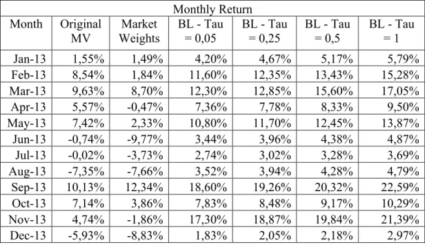
Table 5.1 Monthly Retuns ... 49 Table 5.2 Monthly Sharpe Ratio ... 50

(11)

FIGURES

Figure 2.1 Normal Distribution ... 9

Figure 2.2 Efficient Frontier ... 13

Figure 2.3 Capital Allocation Line ... 17

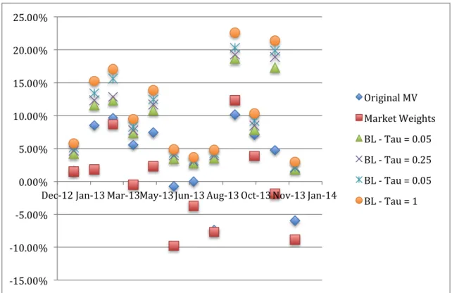
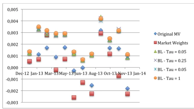
Figure 5.1 Monthly Return Of Each Strategy ... 51

(12)

ABBREVIATION MV : Mean-Variance

BL : Black-Litterman

GARCH : General Autoregressive Conditional Heteroskedasticity EGARCH : Exponential GARCH

(13)

SYMBOLS

Return of asset 𝑖 : 𝑟_!

Variance of asset 𝑖 : 𝜎_!!

Standard deviation – Volatility of asset 𝑖 : 𝜎! Covariance between assets 𝑖 𝑎𝑛𝑑 𝑗 : 𝐶𝑜𝑣(𝑖, 𝑗) Correlation coefficient of assets 𝑖 𝑎𝑛𝑑 𝑗 : 𝜌_!,!

Risk Aversion : 𝛿

(14)

1.INTRODUCTION

One of the major concerns in investment literature is to find out the best way to allocate the assets. All investors concerned about how to select optimal portfolio that fulfill the investment objectives over the investment horizon. Asset allocation is a complex process for couple of reasons. Great number of opportunities to invest-in and inability to prognosticate the future are obstacles of this process. Aside from the many different investment opportunities that are available, nowadays information technology and world wide connections make it easy to invest whether in domestic opportunities or in an international project. For instance it is possible to invest European Markets and Emerging countries simultaneously. Investment is always a risky concept. Initial Investment is made for certain amount of money, but it is never certain about value of return in future. Furthermore, it is impossible to forecast future financial and economic events with certainty. These two problems make it difficult to have optimum and certain asset allocation.

Fundamentally there are two methods in portfolio selection, heuristic and quantitative. In heuristic method, asset allocation is made just with investor feeling and point of views about future performance of the investment that he or she collected from the news and media. This type rarely relies on a model. On the other hand, quantitative approaches apply a mathematical model in portfolio selection process. The model evaluates the investments and determines which one should select in process.

Due to the scarcity of resources as one the basic rules of the economics, all economic and also financial decisions are made in the context of trade-off. The main quantitative model provided by Harry Markowitz (1952). He recommends that in asset allocation process should not only look at the possible pay-off of the investment, but also take into account how certain one is that this payoff will actually be acquired. Markowitz identified the trade-off facing the investor: risk versus expected return. The investment decision is not necessarily which securities to buy, but how to divide the wealth amongst securities. In that article and subsequent works, Markowitz extended the techniques of linear programming to develop the critical line algorithm. The critical line algorithm identifies all feasible portfolios that minimize risk, as measured by variance or standard deviation, for a given level of expected return or maximize expected return

(15)

for a given level of risk. When graphed in standard deviation versus expected return space, these portfolios form the efficient frontier. The efficient frontier represents the trade-off between risk and expected return faced by an investor when forming his or her portfolio. The intuition behind the efficient frontier represents well-diversified portfolios. By this reason diversification plays an important role for achieving risk reduction in portfolio concept. Therefore, mean-variance model gives precise analysis of mathematical meaning to the common proverb “Don't put all of your eggs in one basket.” Markowitz developed mean-variance analysis in the context of selecting a portfolio of common stocks. Over the last decades, mean-variance analysis enormously used in applied asset allocation. By formulating agued issues he proposed the Mean-Variance optimization process. Mean-variance model requires not only knowledge of the expected return and standard deviation on each asset, but also the correlation of returns for each and every pair of assets. Whereas a stock portfolio selection problem might involve hundred of stocks and then thousands of correlations, an asset allocation problem typically involves a bunch of asset classes i.e. stocks, bonds, real state and derivatives. Furthermore, the opportunity to reduce total portfolio risk comes from the lack of correlation across assets.

One might expect mean-variance model currently plays a dominant role in assets allocation process. However, this is not happening completely. Although this model inspired a rich field of science and used by many, it has couple of weak points. Firstly, the utility maximization process of Markowitz is highly sensitive to the input data set. Small changes in the estimated returns or volatilities can result in drastic changes in the final allocation. Secondly, the investors may have their estimations about future returns in hand and want to impose them in the optimization process. An investor may have different subjective views for some of the assets in addition to estimations coming from a quantitative model. He or she wants to merge the feelings with the estimated return came from quantitative model.

For more explanation, the input values for this model are estimated and the optimization procedure assumes that they are true specifications of assets. However, future returns are random variables and their true values differ from their expected values. Commonly, mean-variance optimization process results in extreme short sale positions or minus weights. However if portfolio weights are bounded between zero and one, majority of

(16)

assets take the zero weights and only a few will be incorporated into the optimal portfolio. Furthermore, if the parameters estimated correctly, the resulting portfolio weights obviously lead to the highest preference level. In contrast, if the parameters deviate from the forecast, the poorly diversified portfolio could achieve a poor preference level. By the same way, the optimal weight vector is very sensitive towards input parameters. Small changes in expected returns can result in large variations of portfolio weights.

These deficiencies encountered when using the Mean-Variance optimization in the real investment situation, motivated Black Fisher and Litterman Robert to develop better models on asset allocation. Black and Litterman while analyzing investment portfolios in Goldman Sachs, provided a model to combine Heuristic approach & Quantitative approach (1990). The first publication on the model was in 1990, and subsequently in 1991, 1992. Their proposed model allows investor to incorporate his or her feelings and views on optimization process. The difference between two main models, is rather than applying investors expected returns of all assets into the formula of the Markowitz Model to get optimal portfolio directly, the Black-Litterman Model defines a view portfolio, which specifies investors expected returns of some assets and the degree of confidence in each view. Based on this view portfolio, market equilibrium returns are adjusted to express views of investors. Instead of the view portfolio, the adjusted market equilibrium returns -the new Combined Return in Black-Litterman formula- is applied into the Markowitz Model to get optimal portfolio. The core idea of their model is to use market equilibrium as a neutral reference and then adjust equilibrium values in accordance with an investor’s views to get the optimal portfolio for the investor. They simply use the CAPM equilibrium as the initial reference point and blend this prior information with the subjective analyst views in accordance with the confidence level of the investor about these views.

The traditional manager may form views from news about performance of companies, markets, interest rates and currencies. A view could be that Food industry will outperform Automobile industry. More over the view may also be that the Turkish companies will outperform Swedish companies or Arçelik will outperform Vestel. Using these views without a quantitative model, may have limited help in portfolio

(17)

construction. Usually traditional investors, with lack of mathematic background, are reluctant to use quantitative models, as they feel that techniques of mean-variance analysis and related procedures do not produce value-added effectively. In contrast, the quantitative investor just uses the extreme mathematical methods to capture more return from portfolio. The Black-Litterman model integrates these two approaches and allows traditional investors to express their views and forecasts to consider in a quantitative model, to produce optimum portfolio with both viewpoints.

Black and Litterman (1990) (1991) emphasized on two strengths of their approach: First, they believe that the subjective views of the investors can be easily incorporated in the portfolio construction process. Secondly, their mean-variance optimization does not generate unreasonable solutions, as the original mean-variance framework does. The former point emerges from the feature of the model that investors’ subjective views are expressed as linear combinations of expected returns of assets, rather than as expected returns of individual assets. That is, the subjective view need not be an exact value of the expected return of an individual asset, but rather can be expressed as the expected return of two assets or more in relation to each other. This type of formulation is easier for investors to apply. The later point comes from the feature that the investors’ subjective views are bended with an equilibrium model that tilts the portfolio weights away from the market capitalization weights based on the relative uncertainty in the investor’s views.

Despite numerous advantages of Black-Litterman model, which overcome drawbacks of the original Mean-Variance optimization, specifications of inputs were less straightforward. In other words, the initial publications were written on intuition and proof of formulas on their proposed model. Scowcroft & Satchell (2000) and Idzorek (2004), published their studies on demystification and step-by-step guide to apply Black-Litterman model in real world portfolios.

The Black-Litterman model provides the flexibility of combining the market equilibrium with additional market views of the investor. In the Black-Litterman model, the user inputs any number of views or statements about the expected returns of arbitrary portfolios, and the model combines the views with equilibrium, producing both the set of expected returns of assets as well as the optimal portfolio weights. In practice,

(18)

Black-Litterman model requires two sets of data to input. The first set of comes from CAPM equilibrium expected returns and historical variance-covariance, same is used in Original Mean-Variance optimization. The second one and the most significant set used in application of that model is to construct a vector of views on assets’ expected rate of return.

The analyst may have views on all of the assets or construct a vector of views for selected assets. Investment analysts track the stock’s behavior, markets, general economy criteria, news etc. and apply the realities in fundamental and technical analysis to make prognostication on future returns. In contrary, the model also could be used with quantitative forecast of assets either. Initially, Beach and Orlov (2007) suggested using GARCH models to create inputs for Black-Litterman model. Martellini and Ziemann (2010) include non-normally distributed returns and consider fat tails, to apply the model in special financial instruments i.e. hedge funds and derivatives.

The purpose of the research is to test the performance of the portfolios obtained from the Original Mean-Variance and Black Litterman models over a 5 year period. For former model it uses utility function for building optimum portfolio weights. For later model, it applies reverse optimization to construct the initial equilibrium returns as a neutral starting point, then uses estimation of the variance matrix for views as described in Walters (2007).

One of the features of this study, is the use of EGARCH derived views as proxies for investor views for the Black-Litterman model. Similarly, as Beach and Orlov (2007), however, forecasting the return for each asset has done individually. EGARCH-mean forecasting applied for each of the stocks in univariate context. The benefit of employing this model is that more objective views are obtained, i.e. they are not dependent on the subjective projections of the portfolio manager. In addition, GARCH type models are able to capture characteristics of stock returns. The outcome of this paper should be interesting both for private portfolio managers and institutions participating in Turkish market, and who wants to use an objective methodology for predictions of future returns and volatilities.

(19)

BL model and explores the behavior of Black-Litterman’s results for different valued of Factor Tau, which is used to scale the investors uncertainty in their prior estimate of the returns.

As outline of this thesis, the first chapter gives a theoretical background and notation that will be used. In second chapter it moves to the basis of portfolio selection with the model of Markowitz and the subsequently developed capital asset pricing model. Furthermore, it will discuss the focus of this thesis: the Black-Litterman model. Next chapter will review related recent literatures. Afterward data specification and methodology of this thesis will be described in forth chapter. Chapter five will discuss empirical findings and results. Eventually conclusion and further studies will be included in the last chapter.

(20)

2. THEORETICAL FRAMEWORK

The study of asset allocation process has its own vocabulary. The most important vocabulary and concepts and notation will be discussed in this chapter. In addition, background of two portfolio optimization models will be explained later.

2.1 ASSET PROPERTIES

Terms used in this part are derived from Dictionary of Finance and Banking. (2008) 2.1.1 Classes

An investor can choose from wide variety of different assets. These opportunities can be divided in classes of assets with the same characteristics. The most well known asset class is equity. Equity or stock is the ownership of a part of a company. Equity of public companies can be traded on a stock exchange. Another asset class is fixed-income securities, also known as bonds. A bond is debt investment in which an investor loans money to an entity that borrows the funds for a defined period of time at a fixed or variable interest rate. Bonds used by companies, municipalities, governments to finance variety of projects and activities. Bonds, as every investment, vary in the degree of risk attached to them. The length of the borrowing period and the entity that issues the bonds are important risk factors. Short-term government bonds are generally regarded as very safe investments and generally referred to risk-free investment. The final class under consideration is cash equivalents. It derives from investing in foreign currency, either to bet on a change in the exchange rate or to insure, or hedge, investments in that currency against changes in the exchange rate.

2.1.2 Expected Return And Risk

The motivation behind investment in assets is to get profit in future. The ratio of profit or value-added to initial investment is known as the rate of return. Return defined for a period in the past, but in portfolio selection investor interested in the future behavior of an asset. Markowitz (1959) agues the future or forecasted return as expected value of the return. If rt known as the return of asset up to time t, Expected Return or 𝐸 𝑟 is shorthand of 𝐸(𝑟_!!!| 𝐼_!) which means the forecast of the return at time 𝑡 + 1 given all

(21)

information up to and including time t. The expected return is on of two important characteristics of an asset for mean-variance optimization. Risk is the next important property of an asset for evaluation in portfolio selection process. By definition, risk is the chance to loose on an investment. Markowitz (1952) defined the risk quantitatively by variance of return over a period. Variance measures deviation around a point, so in case of investment deviation of return around expected return. Therefore in mean variance optimization process for an asset, investor should consider its Expected Return and its Risk, measured in variance.

Expected Value: The expected value also known as population mean and defined as the average value of sample and generally denoted by 𝜇.

𝐸 𝑥 = 𝜇 =

1 𝑛

𝑥

!

!!!

Variance : The variance is a measure of how much variable varies around expected value µ. Variance is denoted by 𝜎!_.

𝜎

!

₌

1 𝑛

(𝑥

!

− 𝜇)

!

!!!

Standard Deviation: The standard deviation (𝜎), is square root of the variance, in finance it is often called volatility. Since standard deviation is directly related to normal distribution, it is more intuitive measure of variability than variance.

Covariance The covariance provides a measure of the degree to which returns on two risky assets move in tandem. A positive covariance means that asset returns move together. A negative covariance means returns move inversely. Covariance between asset 𝑖 and 𝑗 is denoted by 𝐶𝑜𝑣(𝑖, 𝑗).

𝐶𝑜𝑣 𝑖, 𝑗 =

1 𝑛

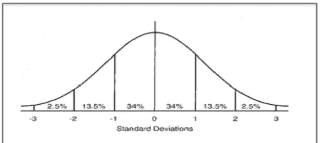
Normal Distribution In finance, it is assumed that the distribution of the asset returns have normal distribution, e.g. by Black & Litterman (1991)

Figure 2.1 Normal Distribution

_!

)

! !!!

= 𝒘

!

_{𝐸 𝑟}

𝑣𝑎𝑟 𝑟

_!

= 𝑣𝑎𝑟

𝑤

_!

𝑟

_! ! !!!

=

𝑐𝑜𝑣 𝑤

_!

𝑟

_!

, 𝑤

_!

𝑟

_! ! !!! ! !!!

=

=

𝑤

_!

𝐸(𝑟

_!

)

! !!!

=

1 𝑛

𝐸 𝑟

! !!!

= 𝐸 𝑟

Thus, the expected return of a portfolio in this equation in independent of the number of assets in the portfolio. However, the variance of portfolio return depends on the number

Obviously by increasing the number of uncorrelated assets in a portfolio, the volatility of portfolio gets closer to Zero:

lim

!→!

𝑣𝑎𝑟 𝑟

!

= lim

!→!

𝜎

!

𝑛

= 0

2.2 THE MARKOWITZ MEAN-VARIANCE OPTIMIZATION

In contemporary history of finance Markowitz’s work plays a significant role in investment. Mean-Variance model is still basis for quantitative asset allocation. This optimiztion holds for Black-Litterman model, as well. Therefore, there would be an in-depth study of Mean-Variance model. In this chapter we are going to discuss model development and mathematics of Mean-Variance. Capital Asset Pricing Model can be used to determine expected return of an asset. CAPM will be discussed, too.

2.2.1 Model Evolution

To develop an investment model there should be an idea of the way which investor select a portfolio. Although majority of investors follow the news and economic conditions to form views and make prediction on future performance of markets, sectors and specific companies, however, these views alone is not enough to do asset allocation. The better way to select portfolio is to use quantitative models. Quantitative models can guide investors to asset allocation. In addition to its inputs, like other quantitative models portfolio selection model needs an objective function.

To make an objective function we should consider that investor aims to make positive return on the investment. Therefore, expected return function is an objective function. To have maximized expected return portfolio we can simply invest in a single asset portfolio with the highest expected return. However, it is against the concept of

(25)

diversification. When the performance of portfolio solely depends on the one asset this makes expected return very risky. On the other hand, monitoring and measuring risk in portfolio selection is other part of objective function. Diversification leads the portfolio to more steady expected return and acceptable risk. An investor that only takes on additional risk in trade-off between risk and return for additional expected return is called risk averse investor. Risk aversion is taken to best description of human investment behavior.

Markowitz Harry Markowitz (1952), identified the forecasted return with expected return and risk with variance of return. He went on to suggest that the above objective is the one to strive for and developed a mathematical model for portfolio selection. The objective, in terms of variance becomes to minimize the variance of return for a certain level of expected return. The expected value is often called the mean value. Therefore, this kind of optimization is Mean-Variance (MV) optimization. He defines a portfolio that minimizes variance for a certain level of expected return, or equivalently maximizes variance for a certain level of variance an efficient portfolio (Markowitz, 1987).

Utility Theory basically categorizes the preferences and formalizes the principle of risk aversion. A utility function is a function 𝑢: 𝑍 → ℝ it is a non-decreasing, continuous function that captures the investors preferences. An investor will prefer portfolio 𝑃_! to 𝑃_! if the expected utility of portfolio 𝑃_!_{is greater than the expected utility of portfolio} 𝑃_!. The specific utility function used varies among individuals, depending on their individual risk tolerance and their individual financial environment. The simplest utility function is a linear one u(x) = x. An investor using this utility function ranks portfolios by their expected values, risk does not play a role. The linear utility function is said to be risk neutral since there is no trade off between risk and expected return in the order of preferences. There is wide range of utility functions, however in practice certain standard types are popular. The most commonly used utility functions are Exponential 𝑢 𝑥 = −𝑒𝑥𝑝 −𝑎𝑥 with 𝑎 > 0, Logarithmic 𝑢 𝑥 = log (𝑥), Power 𝑢 𝑥 = 𝑏𝑥!_for 𝑏, 1 and 𝑏 ≠ 0, and the Quadratic function 𝑢 𝑥 = 𝑥 − 𝑏𝑥!_{for 𝑏 > 0. Utility score of a} portfolio not only uses the risk-return characteristics, but also it should take the investor’s risk aversion into account. For simplicity, many practitioners such as CFA

(26)

institute (2012) professionals use 𝑈 = 𝐸 𝑟 −!_!𝛿𝜎!_{, as a general utility function. In this} equation 𝛿 stands for the risk aversion coefficient. Every unit of return is rewarded while every unit of volatility is penalized by the negative sign depending of the degree of risk aversion of the investor.

Efficient Portfolio A set of portfolios with returns that are maximized for a given level risk or vice versa given that there is not any other portfolios with a higher mean and no higher variance or less variance and no less mean. Markowitz (1987) defines Efficient Portfolio as A set of portfolios with returns that are maximized for a given level risk or vice versa given that there is not any other portfolios with a higher mean and no higher variance or less variance and no less mean.

Figure 2.2 : Efficient Frontier

Following the construction of the efficient frontier, the favorite portfolio should be chosen based of investors risk aversion parameter, because different risk aversion levels

(27)

results in various indifference curves. That is to say, assorted investors may select different portfolios from the efficient frontier.

2.2.2 The Mathematics Of The Model

The main idea of mean-variance analysis has been explained in the previous parts. In general, the model should the model should minimize volatility of the portfolio for given level of expected return or maximize the expected return for a certain level of risk. In addition it must consider all weights add up to one. Hereby we review the general model of Markowitz Mean-Variance optimization problem.

𝑀𝑎𝑥𝑖𝑚𝑖𝑧𝑒

𝑤

_!

𝑟

_! ! !!!

1

2 𝛿𝜎

!! 2.2.3 Drawbacks Of MV Optimization 2.2.3.1 Utility theory

The mean-variance criterion makes the exchange between risk and expected return explicit. The criterion states a preference for portfolios with a higher expected return relative to portfolios with a lower level of expected return (for the same level of risk). This seems a reasonable criterion for portfolio selection. However, care has to be taken in applying the criterion, since in some cases the criterion results in unlikely

(28)

preferences.

Hanoch and Levy (1969) analyzed this failure. They analyze preferences with the help of utility theory and subsequently compare these preferences with those obtained from mean-variance optimization. They conclude that in certain cases the preferences resulting from mean-variance optimization differ from those obtained by utility theory. 2.2.3.2 Normally distributed returns

Hanoch and Levy (1969) studied the question when the mean-variance criterion is a valid efficiency criterion for a risk avers investor. An efficiency criterion is said to be valid if it produces the same efficient set for all concave utility functions. The ranking of the elements in the efficient set still depends on the specific utility function. As Tobin (1958) already suspected that the mean-variance criterion is valid if and only if the distribution of the returns is of a two-parameter family. They concluded that the mean-variance criterion is optimal, when the distributions considered are all Gaussian normal. But the symmetric nature of this distribution seems to deny its usefulness as a good approximation to reality, for at least some types of risky portfolios. Even for symmetric distributions, the mean-variance criterion is not valid, when the distribution has more than two parameters.

2.2.3.3 Deficiencies of mean-variance optimization

The theoretical background of mean-variance optimization has been described, in which setting it makes good sense. However, when applying it to real live problems some flaws do arise.

In general diversification is thought of as a reasonable approach to spreading risk. Adding assets to a portfolio that are less than perfectly correlated to the assets already in the portfolio reduces the variance of the portfolio. Black and Litterman (1992) stated the Mean-variance optimization however, can result in portfolios with large long and short positions in only a few assets, which opposes the notion of diversification. If the parameters that are used in the optimization, like the vector of expected return and the covariance matrix, would be known with certainty, it would be reasonable to invest in such concentrated portfolios, but as the expected returns are just forecasts this seems a

(29)

very risky investment choice. Michaud (1989) concentrated portfolios are very counterintuitive, which is one of the reasons for the lack of popularity of using unconstrained mean-variance optimizers in making investment decisions

In A more practical problem is that the model requires input of expected return, variance and covariance of every asset under consideration. If an investor has 1000 assets in her portfolio; it becomes a very cumbersome task to give estimates for all the input parameters. There are solutions to this problem: historical data could be used to give an estimate of the expected return. But historical estimates are often bad predictors of future behavior (Black & Litterman, 1992). Another problem is how the investor should formulate her believes about future performance. Often an investor holds relative views on asset performance, for example that asset a will outperform asset b. Mean-variance analysis needs a specific estimate of the expected return of a single asset and cannot handle relative views.

Furthermore, The model is not robust. This implies that a small change in the values of the input parameters can cause a large change in the composition of the portfolio. The mean-variance model assumes that the input data is correct, without any estimation error. The model does not address this uncertainty and sets out to optimize the parameters as if they were certain. Michaud (1989) describes mean-variance optimizers even as estimation-error maximizer. Best and Grauer (1991) analyzed the behavior of the mean-variance optimizer under changes in the asset mean. They show that a small increase in an asset mean can cause a very different portfolio composition.

2.2.4 The Separation Theorem

_!"!

_{= 𝑐𝑜𝑣 𝑟}

!

, 𝑟

!

= 0

𝜎

_{!"# !""#$#%&'}

= 𝑤

_!

𝜎

_!

Figuer 2.3 : Capital Allocation Line

(31)

Separation. All investors purchase the same portfolio of risky assets where the line from Risk-Free point touches the Efficient Frontier at the highest Expected Rate of Return possible. Because investors can borrow or lend at the risk-free rate, they move along the new line called, Capital Allocation Line. Alternatively, more risk-averse investors will lend funds and achieve a lower rate of return. And vice versa, less risk-averse investor will borrow fund and achieve a higher rate of return. But because of separation, each investor holds the same portfolio of risky assets.

2.3 CAPITAL ASSET PRICING MODEL

The Markowitz’s study on portfolio selection became relevant with the publication of the Capital Asset Pricing Model (CAPM). William Sharpe (1964), John Lintner (1965), Jan Mossin (1966) and Jack Treynor (1961) worked separately on this theory. CAPM helps the mean-variance analysis of Markowitz to develop a model that can compute the expected return of an asset if equilibrium would exist in the market.

2.3.1 Assumptions

Luenberger (1998) states CAPM model is built based on some assumptions. Under these assumptions, equilibrium can be established in the market. This equilibrium is required to derive the pricing formula:

a) All investors use mean-variance analysis to select a portfolio.

b) All investors have homogeneous believes about the future return, variance and covariance of assets.

c) There is a unique risk free rate of borrowing and lending available for all investors. 2.3.2 Equilibrium

From Tobin (1958) separation theorem, it is known that everyone will invest in a single portfolio of risky assets. In addition, investors can borrow or lend at the risk free rate, to adjust the portfolio to the desired risk level. Since everyone uses the same means, variances and covariance, to determine the optimal portfolio, everyone will compile the same risky portfolio. Some investors will seek to avoid risk and will have a high percentage of the risk free asset in their portfolios. Other, who is more aggressive, will have a high percentage of the risky portfolio. However, every individual will form a

(32)

portfolio that is a mix of the risk free asset and the same risky portfolio.

If all investors purchase the same portfolio of risky assets, this portfolio leads to insight underlying the CAPM. As all investors share the same view, and at that moment there is only one optimal portfolio, it will result in a rising price of the assets in the optimal portfolio and hence a downward adjustment of the expected return. The opposite happens with the assets not in the portfolio. These price changes lead to a revision of the portfolios. And this goes on and on, until equilibrium is reached. In this equilibrium the optimal portfolio is the one that contains all assets proportional to their capitalization weights, that is the market portfolio. This means that the market portfolio is mean-variance efficient in equilibrium. The conclusion of the mean-mean-variance approach and Tobin’s separation theorem is that the optimal portfolio, in which everyone invests, must be the market portfolio (𝒘_!).

2.3.3 CAPM Formula

If the market portfolio 𝑀 is mean-variance efficient, this equation holds for the expected return of an asset 𝑖 satisfies the equilibrium:

𝐸 𝑟

_!

− 𝑟

_!

=

(33)

The first part 𝛽_!!_𝜎

!! is called systematic risk. This is the risk associated with the market as a whole. This risk cannot be reduced by diversification because every asset with non-zero beta contains this risk. The second part,var(ϵ!) is termed the unsystematic, idiosyncratic, or specific risk. This risk is uncorrelated with the market and can be reduced by diversification. It measured by beta, that is most important, since it directly combines with the systematic risk of other assets. A result of CAPM is that expected return depends on this beta. On other hand, strong assumptions of CAPM, make this model poor. For example, to reach the real market portfolio non-tradable assets should be included. In addition, since different investors may use various methods to estimate the expected returns they all may not have homogeneous expectations. However, CAPM is an effective equilibrium, if it can be combined with active methods such as Black-Litterman, it may become more functional in an investment decision process. CAPM can provide a solid reference path while the oscillations from this path can be captured by the active methods. Probably this is the main reason of preferring CAPM as the prior model in the original paper of Black and Litterman.

2.4 THE BLACK-LITTERMAN MODEL

The original mean-variance model was an innovative model in portfolio selection. It guides investors to allocate asset quantitatively in their portfolio. But as explained in the previous part, the model has its deficiencies. Investors who make use of this model may face many limitations. The mean-variance model unrealistically requires expected returns of all assets as input data. For investors, it is almost impossible to know expected returns with certainty. Even for portfolio managers, reliable return forecasts are only available for a small subset of assets. Drobetz & Köhler (2002) discuss while it is impossible to accurately predict the returns of all assets in practice, results of the Markowitz Model are very sensitive to small changes in expected returns. Small changes in expected returns can cause remarkable changes in the optimal portfolio weights. In addition, the MV model usually leads to extreme portfolio weights, which are unreasonable to be implemented in investors’ portfolios. Black and Litterman (1990) describe when running the model without constraints, it almost always recommends portfolios with large negative weights in several assets; when optimizing a portfolio with constraints, the model gives a solution with zero weights in many of the

(34)

assets and therefore takes large positions in only a few of the assets. Moreover, Mankert (2006) states the mean-variance does not distinguish strongly held views from vague assumptions. Therefore, the optimal portfolio weights have no intuitive relation with the views investors actually wish to express.

2.4.1 Model Background

Initially Fischer Black and Robert Litterman, (1991) (1992) whilst working at Goldman Sachs Investment Company, initially proposed to improve the MV model. They ask some investors’ perspective to develop a model that could be used to Goldman Sachs for portfolio selection. They made their portfolio selection model by considering invertors’ feeling and views on the market. They have published some articles for their proposed model, However, none of them were describe the mathematics of the model precisely. Thereafter couple of researchers tried to clear the ambiguity of the model. Satchell and Scowcroft (2000) attempted to demystify BL’s math model in their study. Lee (2000) made a short description of the model in the tactical asset allocation. Idzorek (2004) provides a comprehensive review of all the articles on the model and describes a new method for setting conditions.

Black and Litterman tried to build a more intuitive portfolio by computing a better estimate for the expected return vector. Then use this vector directly for better asset allocation in mean-variance optimizer. They identified two sources of information about the expected returns and they combined these two sources of information. The first source of information is obtained quantitatively, i.e. from CAPM if the market is in equilibrium. The CAPM returns form a frame to the modeling procedure, and use to modify extreme views of the second source of information. The second source of information is the point views and feelings of the investor. The investment manager has access to various information centers and may have different ideas about the market equilibrium. The main idea of BL model is to combine these to two sources of information, which results in a new vector of expected returns. This improved vector of expected returns leads to better asset allocation in portfolios.

The Black-Litterman original model (1991) uses an international index such as S&P 1200 as a proxy to reflect global benchmark in CAPM, to compute the equilibrium

(35)

returns in global context. In addition, investor has views on the expected return of assets. The BL-model allows investors to express their views in an absolute sense, as well as in a relative sense. For example asset 𝑋 will have an expected return of 𝑟, or asset 𝑋 will outperform asset 𝑌. Expressing views in relative way is much closer to investor’s feelings. Furthermore investor may not equally certain about every view. The model made it possible to considers a level of certainty to each view separately. The number of views of investor on about the asset is flexible. It ranges from no view at all, to as much views as there are assets to invest in. This makes the model much better to use. It is important to note that the process of specifying views about the assets in the investment universe is not a compulsory job. The investor may provide the model with no views, one view or one hundred views but is never obliged to provide a view for every asset class. This fact separates the Black-Litterman model from the classic mean-variance approach. Intuitively, it offers a great strength since it is implausible to assume that the investor can express a particular view for every asset class in the investment universe at all times.

The view specification process relies on two assumptions. Walters (2007) explains: first, that each view is unique and uncorrelated with the other views and second, that each view is fully invested so that the sum of weights in a view is zero if the view is relative or one if the view is absolute. Investors often focus only on a small part of the potential investment universe, choosing assets that they feel are undervalued, finding assets with positive momentum, or identifying relative value trades. In Black-Litterman model, it is only necessary to specify a view if the investor holds one. Different authors use different weighting schemes for the view matrix. Satchell and Scowcroft (2000) used an equal weighting scheme on the other hand. He and Litterman (1999) use a market capitalization-weight scheme. Idzorek (2004) argues that the method used by Satchell and Scowcroft may result in undesired and unnecessary tracking error. Instead, he suggest using the market capitalization scheme which means that the relative weighting of each asset in the P matrix will be proportional to that assets market capitalization divided with the whole market capitalization of either the outperforming asset or the underperforming asset. Consequently, views on small cap assets will receive a smaller relative weight than large market cap assets.

(36)

2.4.2 The Mathematics Of Model

Having discussed in previous parts, the Black-Litterman model assumes that there are two sources of information about the expected returns; market equilibrium and investor views. Both sources of information are assumed to be uncertain and are expressed in terms of probability distributions. The main challenge of this model for building one vector of expected returns is to merge these sets of information. Empirically, investors may combine the expected returns with their feelings heuristically. For example if investor has positive feelings regarding an asset, then simply increase the weight of the asset in portfolio, and vice versa for assets with negative outlook may decrease its share. Thereafter the amount of increase or decrease would be asked. Furthermore, assets may correlated: if one asset is expected to do well and therefore the weight is increased, then the weights of other positively correlated asset should also be increased. It would be very complicated to do this all by hand. Black and Litterman (1991) combined these two separate sources of information in a constructive manner and suggested two methods to accomplish this. First, the mixed estimation method of Theil (1971) which is related to the generalized least square method to estimate dependent parameters. Secondly, they suggest that the new vector of expected returns should be “assumed to have a probability distribution that is a product of two normal distributions”.

In these studies, not only the mathematical method to compute the combined vector of expected returns is crudely described, but also the characteristics of the variables are debatable. Litterman (2003) shows that even the view is not related to the third asset, the corresponding weight is affected by the views, depending on the covariance structure among the assets. Although there are brief discussions about the estimation method and the variables, the full setup is not given in a clear and detailed manner. Intermediate steps and the derivations are also absent in the paper. Therefore, to keep simple, the mathematical procedure will be summarized in a different notation than the original papers.

Meucci (2010) describes Theil’s mixed method in Black-Litterman application. For two sources of information they assign 𝝅 = 𝛿Σ𝐰! to equilibrium excess returns with the risk element of 𝜏Σ, and 𝑄 to the investor views, with the risk element of Ω . Investors derive these expected returns by a common factor 𝐄(𝐫) .

(37)

𝝅 = 𝐼 . 𝐄(𝐫) + 𝑢

𝑄 = 𝑃. 𝐄(𝐫) + 𝑣

𝐼 is the identity matrix,

𝑢 is the error term with mean of zero and variance of 𝜏Σ 𝑃 is the matrix corresponding views

𝑣 is the error term with mean of zero and variance of Ω 𝛑 ~ 𝑁 𝐼 . 𝐄(𝐫) ; 𝜏Σ

𝑄 ~ 𝑃. 𝐄(𝐫) ; Ω

With Theil’s mixed estimation, two equations are consolidated to estimate the common factor 𝐸 𝑅 :

𝛑

𝑄 =

_𝑃

𝐼

. 𝐄(𝐫) +

𝑢

_!"

= 𝜏Σ

!!

_{+ 𝑃′Ω}

!!

_𝑃

!!

The formula derivation omitted in this study , however it can be found in Idzorek’s step by step guide (Idzorek, 2004).

𝜇!" is the new(posterior) combined vector 𝜏 is a scalar

Σ is the covariance matrix of excess returns

(38)

Ω is a diagonal covariance matrix of error terms from the expressed views representing the uncertainty in each view

𝛑 is the implied equilibrium vector

𝑄 is the vector of view in terms of relative or absolute changes

By applying the new combined return (𝜇_!") into Markowitz model optimal portfolio weights are solved.

It is unclear what the parameters represent and how they should be specified. This makes model very confusing to use. Of the two approaches suggested by Black and Litterman the most widely used approach is the Bayesian one, especially after the publication of an article by Stephen Satchell and Alan Scowcroft (Scowcroft & Satchell, 2000) about the derivation of the BL formula. They use Bayes’s Probability Density Function to merge the views of the investor with equilibrium expected returns.

They assumed investor has 𝑘 < 𝑛 views, expressed as a linear relationship

𝑃𝐄(𝐫) = 𝑄 + 𝝐

Where 𝑃 ∈ ℝ!×!_{,𝑄 ∈ ℝ}!_,_{𝝐 ∈ ℝ}!_{~𝑁(0, Ω) and Ω ∈ ℝ}!×!_{is a diagonal covariance} matrix. Here, 𝑃 is the matrix that identifies the asset involved in the views, 𝑄 is the vector of view in terms of relative or absolute changes, 𝝐 is the uncertainty of the views, 𝐄(𝐫) is an unknown vector and needs to be estimated from equilibrium. Bayes’ Theorem is mathematically not very challenging. To apply the theorem to the problem at hand is less straightforward. Here to distinguish between notations, 𝒫 represents the probability density distribution of Bayesian theorem. It is assumed that the investor forms his or her views using knowledge of the equilibrium expected returns 𝛑. Therefore, the equilibrium expected returns are considered the prior returns and these will be updated with the views of the investor. The posterior distribution combines both sources of information. Using Bayes’ formula in this context yields:

𝒫 𝑃𝐄 𝐫 |𝛑 =

𝒫 𝛑|𝑃𝐄 𝐫 𝒫 𝑃𝐄 𝐫

𝒫 𝛑

(39)

!!

_𝑄

Σ

_!"

= 𝜏Σ

!!

_{+ 𝑃′Ω}

!!

_𝑃

!!

The formula derivation proof could be found in demystification of the Black–Litterman (2000).

2.4.2 Expressing The Views

As discussed in previous part, the major challenge of Black and Litterman model is to incorporate the quantitative expected returns and views of the investor. Main part of the job is expressing views. Idzorek (2004) emphasized that the investor can express relative views, for example that asset A will outperform asset B by 2%. This manner of expressing is an important improvement of the BL-model over traditional mean-variance optimization, as this manner of expressing views is more intuitive than expressing absolute views.

Let us move to the mathematical description of the manner of expressing views and the view matrix P. An investor often holds views about performance of assets, asset classes or markets. The mathematical representation of these views needs to meet a few

(40)

characteristics. The views have to be specified relative to the vector of expected return E(r), the views have to be specified relative to each other and it has to be possible to express a level certainty in the view. These prerequisites lead to the following specification.

𝑃𝐸(𝑟) = 𝑄 + 𝜀 𝑤ℎ𝑒𝑟𝑒 𝜀~𝑁(0, 𝛺),

𝑃 ∈ ℝ!×!_{in known , 𝑄 ∈ ℝ}!_{in known, 𝜀 ∈ ℝ}!_{is and error vector with know variance}

Ω ∈ ℝ!×!_{, 𝐸(𝑟) ∈ ℝ}!_{in unknown and needs to be estimated.}

Assets that are under consideration can be specified in the matrix 𝑃, the vector 𝑄 expresses the relative change in performance and the vector of random variables 𝜀 expresses the uncertainty of the view. The vector 𝜀 is normally distributed with mean zero and variance Ω. That the mean is zero means that the investor does not have a standard bias against a certain set of assets. It is assumed that the views are mutually uncorrelated and therefore the covariance matrix Ω is diagonal. A variance of zero represents absolute certainty about the view. The vector 𝐸(𝑟) is the unknown expected return vector that needs to be estimated. What is often not noted is that Black and Litterman let the manner of formulating views in the matrix P completely free, they not did give any characteristics. Scowcroft & Satchell (2000) described a more general idea about expressing views on a portfolio of assets. Then the matrix P is considered as a series of portfolios and the vector 𝑄 holds the expected return of the corresponding portfolio. It is difficult for a person to estimate the expected return of a portfolio of assets. However, this more general definition does capture all manners of expressing views.

A portfolio could exist of one asset, which would correspond to expressing an absolute view on an asset; a portfolio could be zero-investment, this would correspond to expressing a relative view, and finally one has the possibility to express views on more than two assets. It is important to note that the vector 𝑄 denotes the forecasted relative performance of the assets.

An example can make this manner of expressing views more clear. There is four class of assets to invest:

(41)

I.Turkish Treasury Bonds

II. Real State Investment Trust (REIT) III. Borsa Istanbul (BIST)

IV. International Bonds V. Euro Bonds

Here investor could have view with maximum number of four. Suppose investor made relative and absolute views in this respect:

View 1 : REITS will have absolute return of 2.5% View 2 : BIST will out perform REIT by 5 %

View 3: Turkish Bonds will outperform International Bonds and Euro Bonds By 3 % This views can express in matrices in following way:

0

1

0 0 −1 1

1

0

0 −0.5 −0.5

𝐸 𝑟 =

2.5%

5%

3%

+ 𝜀

Obviously, there is 3 rows and 5 columns in matrix 𝑃. Each row belongs to one view. The first view which is an absolute view , related asset is REIT , thus it tak e the value of 1 and other take zero. Second view expressed in relative form, the outperformer take the value of 1 and denominator takes -1. For the last view which is also stated in relative for the Turkish Treasury Bonds, take the value of 1 , then International Bonds and Euro Bonds take the value of -0.5 equally. There is a significant point in dividing denominator assets. Here equally spreading is used. However, Market Capitalization weights could be used , as well. Matrix 𝑃, which is called the Link Matrix, links the views to corresponding assets.

In vector 𝑄, there is two rows for each view. Therefore the first view 2.5% places in first row and 5% in second one respectively. So views will have a vector of 𝑛×1, 𝑛 as the number of views. The next matrix in the link matrix which links the views to the asset. After constructing the 𝑃 𝑎𝑛𝑑 𝑄 matrices the remainder is just to put these value in BL combining formula.

(42)

2.4.2 The Factor Tau

The factor 𝜏 (Tau) is probably the single most confusing aspect of the Black-Litterman model. Many authors use different values, or just ignore it. Christodoulakis (2002) states originally it is used to specify the relation between the distribution of the asset returns and the distribution of the mean of the asset returns. Walters (2007) 𝜏 is used to scale the investors uncertainty in their prior estimate of the returns. There are several different approaches to calibrating it, or even including it described in the literature. Just to illustrate the difference of opinion, here is comments from three authors. He and Litterman (1991) set 𝜏 on 0.05. Satchell and Scowcroft (2000) state that many people use a value of τ around 1. Koch (2005) on the other hand takes a position somewhat in the middle and finds that values of τ = 0.3 are reasonable. All these differing opinions require an investigation into the value of τ. Meucci (2010) proposes a formulation of the Black-Litterman model without 𝜏. The main difference between the original reference model and other reference models is uncertainty. The posterior estimates include an updated covariance matrix. This model requires the investor to estimate an additional parameter τ which impacts the posterior covariance matrix as well as the estimated returns.

2.4.3 Following Studies On The Basic Model

He and Litterman (1999) proved a computationally more stable version of the posterior mean and covariance. Both the Original Reference Model approach used in Black and Litterman (1991) and He and Litterman (1999) and the Alternative Reference Model approach used in Satchell and Scowcroft (2000) is mathematically described in vague manner. Idzorek (2004) offers step-by-step instructions for practitioners to the Black-Litterman approach. Meucci (2010) discusses the original reference model and made comments on the first of two extensions made by Satchell and Scowcroft mentioned above and argues that Factor Tau should be set between 0 and 1 in practice rather than using the extension. Author described posterior distribution building on the formulas derived by He and Litterman (1999) and used in the original framework presents two puzzles, when views are stated with extreme confidence so that the variance of the views goes to infinity or zero, in other words investor confidence in views are zero or 100%. Walters (2007) presents a complete walkthrough and derivations of the