EUROPEAN ORGANIZATION FOR NUCLEAR RESEARCH (CERN)
CERN-EP-2020-017 2020/09/18
CMS-JME-18-001
Pileup mitigation at CMS in 13 TeV data
The CMS Collaboration
∗Abstract
With increasing instantaneous luminosity at the LHC come additional reconstruc-tion challenges. At high luminosity, many collisions occur simultaneously within one proton-proton bunch crossing. The isolation of an interesting collision from the ad-ditional “pileup” collisions is needed for effective physics performance. In the CMS Collaboration, several techniques capable of mitigating the impact of these pileup collisions have been developed. Such methods include charged-hadron subtraction, pileup jet identification, isospin-based neutral particle “δβ” correction, and, most re-cently, pileup per particle identification. This paper surveys the performance of these techniques for jet and missing transverse momentum reconstruction, as well as muon isolation. The analysis makes use of data corresponding to 35.9 fb−1 collected with the CMS experiment in 2016 at a center-of-mass energy of 13 TeV. The performance of each algorithm is discussed for up to 70 simultaneous collisions per bunch crossing. Significant improvements are found in the identification of pileup jets, the jet energy, mass, and angular resolution, missing transverse momentum resolution, and muon isolation when using pileup per particle identification.
”Published in the Journal of Instrumentation as doi:10.1088/1748-0221/15/09/P09018.”
c
2020 CERN for the benefit of the CMS Collaboration. CC-BY-4.0 license
∗See Appendix A for the list of collaboration members
1
1
Introduction
At the CERN LHC, instantaneous luminosities of up to 1.5×1034cm−2s−1[1] are sufficiently large for multiple proton-proton (pp) collisions to occur in the same time window in which proton bunches collide. This leads to overlapping of particle interactions in the detector. To study a specific pp interaction, it is necessary to separate this single interaction from the over-lapping ones. The additional collisions, known as pileup (PU), will result in additional par-ticles throughout the detector that confuse the desired measurements. With PU mitigation techniques, we can minimize the impact of PU and better isolate the single collision of interest. With increasing beam intensity over the past several years, identification of interesting pp col-lisions has become an ever-growing challenge at the LHC. The number of additional colcol-lisions that occur when two proton bunches collide was, on average, 23 in 2016 and subsequently in-creased to 32 in 2017 and 2018. At this level of collision density, the mitigation of the PU effects is necessary to enable physics analyses at the LHC.
The CMS Collaboration has developed various widely used techniques for PU mitigation. One technique, charged-hadron subtraction (CHS) [2], has been the standard method to mitigate the impact of PU on the jet reconstruction for the last few years. It works by excluding charged particles associated with reconstructed vertices from PU collisions from the jet clustering proce-dure. In this technique, to mitigate the impact of neutral PU particles in jets, an event-by-event jet-area-based correction [3–5] is applied to the jet four-momenta. Further, a PU jet identifi-cation (PU jet ID) technique [6] is used to reject jets largely composed of particles from PU interactions.
These techniques have limitations when attempting to remove PU contributions due to neutral particles. For the jet-area-based correction, the jet four-momentum correction acts on a whole jet and is therefore not capable of removing PU contributions from jet shape or jet substructure observables. To overcome this limitation, a new technique for PU mitigation, pileup per particle identification (PUPPI) [7], is introduced that operates at the particle level. The PUPPI algorithm builds on the existing CHS algorithm. In addition, it calculates a probability that each neutral particle originates from PU and scales the energy of these particles based on their probability. As a consequence, objects clustered from hadrons, such as jets, missing transverse momentum (pmiss
T ), and lepton isolation are expected to be less susceptible to PU when PUPPI is utilized.
In this paper, the performance of PU mitigation techniques, including the commissioning of PUPPI in pp collision data, is summarized. After a short description of the CMS detector in Section 2 and definitions of the data set and Monte Carlo (MC) simulations used in these studies in Section 3, the CHS and PUPPI algorithms are described in Section 4. In Section 5.1 performance in terms of jet resolution at a high number of interactions is presented. Section 5.2 summarizes the impact on noise rejection of PU mitigation techniques. Section 5.3 presents the rejection of jets originating from PU with PU jet ID and PUPPI. Jets reconstructed with a larger cone size are often used to identify the decay of Lorentz-boosted heavy particles such as W, Z, and Higgs bosons, and top quarks. Pileup significantly degrades the reconstruction performance, and the gain from PU mitigation techniques for such large-size jets is discussed in Section 6. The measurement of pmissT also benefits from PU mitigation techniques, which is discussed in Section 7. Mitigation of PU for muon isolation variables is presented in Section 8.
2
The CMS detector
The central feature of the CMS apparatus is a superconducting solenoid of 6 m internal di-ameter, providing a magnetic field of 3.8 T. Within the solenoid volume are a silicon pixel
and strip tracker, a lead tungstate crystal electromagnetic calorimeter (ECAL), and a brass and scintillator hadron calorimeter (HCAL), each composed of a barrel and two endcap sections.
The ECAL covers the pseudorapidity range |η| < 3, while the HCAL is extended with
for-ward calorimeters up to|η| <5. Muons are detected in gas-ionization chambers embedded in
the steel flux-return yoke outside the solenoid. The silicon tracker measures charged particles within|η| <2.5. It consists of 1440 silicon pixel and 15 148 silicon strip detector modules. For
nonisolated particles with transverse momentum of 1 < pT < 10 GeV and|η| <1.4, the track
resolutions are typically 1.5% in pTand 25–90 (45–150) µm in the transverse (longitudinal) im-pact parameter [8]. A more detailed description of the CMS detector, together with a definition of the coordinate system used and the relevant kinematic variables, can be found in Ref. [9]. The particle-flow (PF) event reconstruction [2] reconstructs and identifies each individual par-ticle in an event, with an optimized combination of all subdetector information. In this process, the identification of the particle type (photon, electron, muon, charged or neutral hadron) plays an important role in the determination of the particle direction and energy. Photons (e.g.,
com-ing from π0 decays or from electron bremsstrahlung) are identified as ECAL energy clusters
not linked to the extrapolation of any charged particle trajectory to the ECAL. Electrons (e.g., coming from photon conversions in the tracker material or from B hadron semileptonic decays) are identified as a primary charged-particle track and potentially many ECAL energy clusters corresponding to this track extrapolation to the ECAL and to possible bremsstrahlung pho-tons emitted along the way through the tracker material. Muons are identified as tracks in the central tracker consistent with either tracks or several hits in the muon system, and associated with calorimeter deposits compatible with the muon hypothesis. Charged hadrons are iden-tified as charged particle tracks neither ideniden-tified as electrons, nor as muons. Finally, neutral hadrons are identified as HCAL energy clusters not linked to any charged-hadron trajectory, or as a combined ECAL and HCAL energy excess with respect to the expected charged-hadron energy deposit.
The energy of photons is obtained from the ECAL measurement, corrected for zero-suppression effects. The energy of electrons is determined from a combination of the track momentum at the main interaction vertex, the corresponding ECAL cluster energy, and the energy sum of all bremsstrahlung photons attached to the track. The energy of muons is obtained from the corresponding track momentum. The energy of charged hadrons is determined from a combi-nation of the track momentum and the corresponding ECAL and HCAL energy, corrected for zero-suppression effects and for the response function of the calorimeters to hadronic showers. Finally, the energy of neutral hadrons is obtained from the corresponding corrected ECAL and HCAL energy.
The collision rate is 40 MHz, and the events of interest are selected using a two-tiered trigger system [10]. The first level (L1), composed of custom hardware processors, uses information from the calorimeters and muon detectors to select events at a rate of around 100 kHz within a fixed time interval of less than 4 µs. The second level, known as the high-level trigger (HLT), consists of a farm of processors running a version of the full event reconstruction software optimized for fast processing, and reduces the event rate to around 1 kHz before data storage. All detector subsystems have dedicated techniques to reject signals from electronic noise or from particles that do not originate from the pp collisions in the bunch crossing of interest, such as particles arriving from pp collisions that occur in adjacent bunch crossings before or after the bunch crossing of interest (so called out-of-time PU). While these rejection techniques are not the focus of this paper, some false signals can pass these filters and affect the PF reconstruction. Particularly relevant is residual noise from ECAL and HCAL electronics that may add to the
3
energy of reconstructed photons, electrons, and hadrons. Algorithms for the rejection of this noise are further discussed in Section 5.2.
3
Data and simulated samples
In this paper, data corresponding to an integrated luminosity of 35.9 fb−1[1] taken in 2016 are used. Figure 1 shows the PU conditions in the years 2016–2018. The number of pp interactions is calculated from the instantaneous luminosity based on an estimated inelastic pp collision cross section of 69.2 mb. This number is obtained using the PU counting method described in the inelastic cross section measurements [11, 12]. In the following sections of this paper, we distinguish between two definitions: “mean number of interactions per crossing” (abbreviated “number of interactions” and denoted µ) and “number of vertices” (denoted Nvertices). Vertices are reconstructed through track clustering using a deterministic annealing algorithm [8]. The number of interactions is used to estimate the amount of PU in simulation. The number of vertices can be determined in both data and simulation. Further details on the relationship between µ and Nverticesare provided in Section 5.3. The studies presented in this paper focus on the PU conditions in 2016, though the trends towards higher PU scenarios with up to 70 simultaneous interactions are explored as well. The trigger paths used for the data taking are mentioned in each section.
Mean number of interactions per crossing 0 10 20 30 40 50 60 70 80 90 100 ] -1 Recorded luminosity [fb 0 1 2 3 4 5 6 in(13 TeV) = 69.2 mb pp σ > = 29 µ 2016-2018: < > = 32 µ 2018: < > = 32 µ 2017: < > = 23 µ 2016: <
CMS
CMS
(13 TeV)Figure 1: Distribution of the mean number of inelastic interactions per crossing (pileup) in data for pp collisions in 2016 (dotted orange line), 2017 (dotted dashed light blue line), 2018 (dashed navy blue line), and integrated over 2016–2018 (solid grey line). A total inelastic pp collision cross section of 69.2 mb is chosen. The mean number of inelastic interactions per bunch crossing is provided in the legend for each year.
Samples of simulated events are used to evaluate the performance of the PU mitigation tech-niques discussed in this paper. The simulation of standard model events composed uniquely of jets produced through the strong interaction, referred to as quantum chromodynamics (QCD)
multijet events, is performed with PYTHIA v8.212 [13] in standalone mode using the Lund
string fragmentation model [14, 15] for jets. For studies of lepton isolation, dedicated QCD mul-tijet samples that are enriched in events containing electrons or muons (e.g., from heavy-flavor meson decays) are used. The W and Z boson production in association with jets is simulated
at leading-order (LO) with the MADGRAPH5 aMC@NLO v2.2.2 [16] generator. Production of
production via the s- and t-channels, and tW processes are simulated at next-to-leading-order
(NLO) with MADGRAPH5 aMC@NLOthat is interfaced withPYTHIA. For Lorentz-boosted W
boson studies [20], MC simulation of high mass bulk graviton resonance [21–23] decaying to
WW boson pairs are generated at LO with MADGRAPH5 aMC@NLO. All parton shower
simu-lations are performed usingPYTHIA. For Z+jets production, an additional sample is generated
using MADGRAPH5 aMC@NLOinterfaced with HERWIG++ v2.7.1 [24, 25] with the UE-EE-5C
underlying event tune [26] to assess systematic uncertainties related to the modeling of the parton showering and hadronization.
The LO and NLO NNPDF 3.0 [27] parton distribution functions (PDF) are used in all generated
samples matching the QCD order of the respective process. The PYTHIA parameters for the
underlying event are set according to the CUETP8M1 tune [28, 29], except for the tt sample, which uses CUETP8M2 [30]. All generated samples are passed through a detailed simulation of the CMS detector using GEANT4 [31]. To simulate the effect of additional pp collisions within
the same or adjacent bunch crossings, additional inelastic events are generated using PYTHIA
with the same underlying event tune as the main interaction and superimposed on the hard-scattering events. The MC simulated events are weighted to reproduce the distribution of the number of interactions observed in data.
4
The CHS and PUPPI algorithms
A detailed description of the CHS algorithm and its performance is found in Ref. [2]. In the fol-lowing, we summarize the salient features and differences with respect to the PUPPI algorithm. Both algorithms use the information of vertices reconstructed from charged-particle tracks. The physics objects considered for selecting the primary pp interaction vertex are track jets, clus-tered using the anti-kT algorithm [32, 33] with the tracks assigned to the vertex as inputs, and the associated~pmiss
T,tracks, which is the negative vector pT sum of those jets. The reconstructed
vertex with the largest value of summed physics-object p2
T is selected as the primary pp
inter-action vertex or “leading vertex” (LV). Other reconstructed collision vertices are referred to as PU vertices.
The CHS algorithm makes use of tracking information to identify particles originating from PU after PF candidates have been reconstructed and before any jet clustering. The procedure removes charged-particle candidates that are associated with a reconstructed PU vertex. A charged particle is associated with a PU vertex if it has been used in the fit to that PU vertex [8]. Charged particles not associated with any PU vertex and all neutral particles are kept.
The PUPPI [7] algorithm aims to use information related to local particle distribution, event PU properties, and tracking information to mitigate the effect of PU on observables of clustered hadrons, such as jets, pmissT , and lepton isolation. The PUPPI algorithm operates at the particle candidate level, before any clustering is performed. It calculates a weight in a range from 0 to 1 for each particle, exploiting information about the surrounding particles, where a value of 1 is assigned to particles considered to originate from the LV. These per-particle weights are used to rescale the particle four-momenta to correct for PU at particle-level, and thus reduces the contribution of PU to the observables of interest.
For charged particles, the PUPPI weight is assigned based on tracking information. Charged particles used in the fit of the LV are assigned a weight of 1, while those associated with a PU vertex are assigned a weight of 0. A weight of 1 is assigned to charged particles not associated
with any vertex provided the distance of closest approach to the LV along the z axis (dz) is
5
corresponds to about 15 standard deviations of the vertex reconstruction resolution in the z direction at an average PU of 10 [8], and it works as an additional filter against undesirable objects, such as accidentally reconstructed particles from detector noise.
Neutral particles are assigned a weight based on a discriminating variable α. In general, the α variable is used to calculate a weight, which encodes the probability that an individual particle originates from a PU collision. As discussed in Ref. [7], various definitions of α are possible. Within CMS, the α variable for a given particle i is defined as
αi =log
∑
j6=i,∆Rij<R0
pT, j ∆Rij
!2(
for|ηi| <2.5, j are charged particles from LV,
for|ηi| >2.5, j are all kinds of reconstructed particles, (1)
where i refers to the particle in question, j are other particles, pT, j is the transverse momentum of particle j in GeV, and∆Rij = √(∆ηij)2+ (∆φij)2(where φ is the azimuthal angle in radians) is the distance between the particles i and j in the η-φ plane. The summation runs over the particles j in the cone of particle i with a radius of R0 = 0.4. A value of αi = 0 is assigned
when there are no particles in the cone. The choice of the cone radius R0in the range of 0.2–0.6 has a weak impact on the performance. The value of 0.4 was chosen as a compromise between the performance when used in the definition of the isolation variable (preferring larger cones) and jet performance (preferring smaller cones). In |η| < 2.5, where tracking information is
available, only charged particles associated with the LV are included as particle j, whereas all particles with|η| >2.5 are included. The variable α contrasts the collinear structure of QCD in
parton showers with the soft diffuse radiation coming from PU interactions. A particle from a shower is expected to be close to other particles from the same shower, whereas PU particles can be distributed more homogeneously. The α variable is designed such that a particle gets a large value of α if it is close to either particles from the LV or, in|η| > 2.5, close to highly
energetic particles.
To translate αi of each particle into a probability, charged particles assigned to PU vertices are used to generate the expected PU distribution in an event. From this expected distribution
a median and root-mean-square (RMS) of the α values are computed. The αi of each neutral
particle is compared with the computed median and RMS of the α distribution of the charged
PU particles using a signed χ2approximation:
signed χ2i = (αi−αPU)|αi−αPU| (αRMSPU )2
, (2)
where αPU is the median value of the αi distribution for charged PU particles in the event
and RMSPUis the corresponding RMS. If signed χ2
i is large, the particle most likely originates
from the LV. The sign of the numerator is sensitive to the direction of the deviation of αi from
αPU. For the detector region where|η| >2.5 and tracking is not available, the values αPUand
RMSPUcan not be calculated directly. Therefore, αPU and RMSPU are taken from the detector
region where |η| < 2.5 and extrapolated to the region where |η| > 2.5 by multiplying with
transfer factors (see Tab. 1) derived from MC simulation. The transfer factors are necessary, since the granularity of the detector varies with η and leads to a variation of α with η, par-ticularly outside of the tracker coverage (|η| = 2.5) and ECAL coverage (|η| = 3.0). Lastly,
to compute the pT weight of the particles, the signed χ2
i for PU particles is assumed to be
ap-proximately distributed according to a χ2 distribution for χ2
i > 0. The pT weight is given by
wi = Fχ2, NDF=1(signed χ2i)where Fχ2, NDF=1 is the cumulative distribution function of the χ2
distribution with one degree of freedom. Particles with weights wismaller than 0.01, i.e., those with a probability greater than 99% to originate from PU are rejected; this last rejection removes
remaining high-energy noise deposits. In addition, neutral particles that fulfill the following condition: wi pT, i< (A+B Nvertices)GeV, where Nverticesis the number of vertices in the event, get a weight of 0. This selection reduces the residual dependence of jet energies on the num-ber of interactions. The parameters A and B are tunable parameters. To perform the tuning of these parameters, jets clustered from PUPPI-weighted particles in the regions|η| <2.5 and
2.5 < |η| < 3.0 are adjusted to have near-unity jet response, as a function of the number of
in-teractions, i.e., the reconstructed jet energy matches the true jet energy regardless of the amount of PU. In the region|η| > 3, the parameters are chosen such that pmissT resolution is optimized.
Table 1 summarizes the resulting parameters that have been obtained using QCD multijet sim-ulation with an average number of interactions of 23 and a significant amount of events beyond 30 interactions reflecting the 2016 data (orange curve in Fig. 1). The parameters A and B are smaller in |η| < 2.5 (where the majority of particles are reconstructed with the tracker) than
in |η| > 2.5 (where the measurement comes solely from the calorimeters that have a coarser
granularity and thus collect more PU energy per cell).
Table 1: The tunable parameters of PUPPI optimized for application in 2016 data analysis. The transfer factors used to extrapolate the αPUand αRMSPU to|η| >2.5 are denoted TF.
|η|of particle A [ GeV ] B [ GeV ] TF αPU TF αRMSPU
[0, 2.5] 0.2 0.015 1 1
[2.5, 3] 2.0 0.13 0.9 1.2
[3, 5] 2.0 0.13 0.75 0.95
4.1 Data-to-simulation comparison for variables used within PUPPI
The behavior of the variables used in PUPPI has been studied in two complementary data samples. A subset of the data taken in 2016, corresponding to an integrated luminosity of 0.36 fb−1 and selected using trigger paths based on the scalar sum (HT) of the pT of jets with pT > 30 GeV and|η| <3, requiring an offline selection of HT > 1500 GeV, is referred to as the
jet sample. The details of jet reconstruction and performance are discussed in Section 5. Here, we present comparisons of data and QCD multijet simulation based on all PF candidates in the event, rather than clustered jets. As a reference, a data sample enriched in events containing mainly particles from PU collisions is compared with PU-only simulation and is referred to as the PU sample. The PU data sample is recorded with a zero-bias trigger that randomly selects a fraction of the collision events, corresponding to an integrated luminosity of 3.18 nb−1. The distribution of the number of PU interactions in both subsets of data is comparable to the one in the whole data sample collected in 2016.
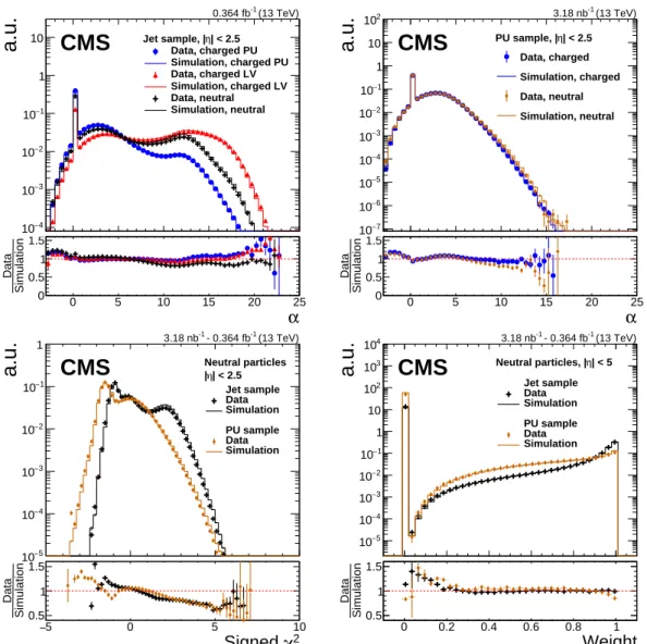
Figure 2 shows the distribution of the three main variables used in PUPPI for data and simu-lation. The upper left plot presents the distribution of α for charged particles from the LV and the PU vertices and for neutral particles with|η| <2.5 in the jet sample. The separation power
of the variable α between particles from the LV and PU vertices for charged particles can be de-duced from this figure. The majority of the charged particles from PU vertices have an α value below 8, whereas only a small fraction of particles have higher values. Charged particles from the LV exhibit a double-peak structure. The first peak at large α is characteristic of particles within jets originating from the LV. The second peak at lower α consists of charged particles that are isolated from other particles originating from the LV. With the exception of particles from lepton decays, which are directly addressed later, isolated particles have limited physics impact and consequently a low α value has a negligible impact on the algorithm performance on physics objects.
4.1 Data-to-simulation comparison for variables used within PUPPI 7
α
a.u.
4 − 10 3 − 10 2 − 10 1 − 10 1 10 Jet sample, |η| < 2.5 Data, charged PU Simulation, charged PU Data, charged LV Simulation, charged LV Data, neutral Simulation, neutral α 0 5 10 15 20 25 Simulation Data 0 0.5 1 1.5 (13 TeV) -1 0.364 fbCMS
α
a.u.
7 − 10 6 − 10 5 − 10 4 − 10 3 − 10 2 − 10 1 − 10 1 10 2 10 | < 2.5 η PU sample, | Data, charged Simulation, charged Data, neutral Simulation, neutral α 0 5 10 15 20 25 Simulation Data 0 0.5 1 1.5 (13 TeV) -1 3.18 nbCMS
a.u.
5 − 10 4 − 10 3 − 10 2 − 10 1 − 10 1 | < 2.5 η | Neutral particles Jet sample Data Simulation PU sample Data Simulation 2 χ Signed 5 − 0 5 10 Simulation Data 0.5 1 1.5 (13 TeV) -1 - 0.364 fb -1 3.18 nbCMS
Weight
a.u.
5 − 10 4 − 10 3 − 10 2 − 10 1 − 10 1 10 2 10 3 10 4 10 | < 5 η Neutral particles, | Jet sample Data Simulation PU sample Data Simulation Weight 0 0.2 0.4 0.6 0.8 1 Simulation Data 0.5 1 1.5 (13 TeV) -1 - 0.364 fb -1 3.18 nbCMS
Figure 2: Data-to-simulation comparison for three different variables of the PUPPI algorithm. The markers show a subset of the data taken in 2016 of the jet sample and the PU sample, while the solid lines are QCD multijet simulations or PU-only simulation. The lower panel of each plot shows the ratio of data to simulation. Only statistical uncertainties are displayed. The upper left plot shows the α distribution in the jet sample for charged particles associated with the LV (red triangles), charged particles associated with PU vertices (blue circles), and neutral particles (black crosses) for|η| <2.5. The upper right plot shows the α distribution in the PU
sample for charged (blue circles) and neutral (orange diamond) particles. The lower left plot shows the signed χ2= (α−αPU)|α−αPU|/(αRMSPU )2for neutral particles with|η| <2.5 in the jet
sample (black crosses) and in the PU sample (orange diamonds). The lower right plot shows the PUPPI weight distribution for neutral particles in the jet sample (black crosses) and the PU sample (orange diamonds). The error bars correspond to the statistical uncertainty.
sample shown in Figure 2 (upper right). It becomes clear that the median and RMS of the α distribution are similar for charged and neutral particles originating from PU. This similarity
confirms one of the primary assumptions of PUPPI, namely that αPU and RMSPU, which are
computed for charged particles, can be used to compute weights for neutral particles with a discrimination power between PU and LV particles. Although the qualitative features of the
α distribution in data are reproduced by the simulation, a disagreement between data and
simulation is observed, which is most pronounced for neutral particles from PU with large values of α.
The χ2distribution shown in Fig. 2 (lower left) shows two peaks for both the jet sample and the PU sample. The first peak results from particles without any neighbor and an α value of zero. The second peak at zero represents all PU particles. The jet sample (black curve) shows a third peak for all LV particles. Additionally, the shape of the resulting PUPPI weight distribution, shown in Fig. 2 (lower right) is well modeled by simulation for particles with high weights (i.e., those likely originating from the LV). A considerable mismodeling is observed at low values of
PUPPI weight, where low-pTparticles from PU interactions dominate. This mismodeling does
not propagate to further observables, because these particles receive small weights, and as a consequence have a negligible contribution. Although both samples have a similar distribution of number of interactions, the weight distribution of the jet sample has more events at higher values of the weight compared to the PU sample because of the selection of a high pTjet.
5
Jet reconstruction
Jets are clustered from PF candidates using the anti-kT algorithm [32] with the FASTJET
soft-ware package [33]. Distance parameters of 0.4 and 0.8 are used for the clustering. While jets
with R=0.4 (AK4 jets) are mainly used in CMS for reconstruction of showers from light-flavor
quarks and gluons, jets with R= 0.8 (AK8 jets) are mainly used for reconstruction of
Lorentz-boosted W, Z, and Higgs bosons, and for top quark identification, as discussed in detail in Section 6. Before jet clustering, CHS- or PUPPI-based PU mitigation is applied to the PF can-didates. Reconstructed jets with the respective PU mitigation technique applied are referred to as CHS and PUPPI jets, respectively.
Jet momentum is determined as the vectorial sum of all particle momenta in the jet, and from
simulation is, on average, within 5 to 20% of the true momentum over the whole pTspectrum
and detector acceptance. For CHS jets, an event-by-event jet-area-based correction [3–5] is applied to the jet four-momenta to remove the remaining energy due to neutral and charged particles originating from PU vertices, while no such correction is necessary for PUPPI jets. Although CHS removes charged particles associated with a PU vertex, charged particles not associated with any vertex are kept and can add charged PU energy to the jet. The remaining energy from PU particles subtracted from the jet energy is assumed proportional to the jet area and parametrized as a function of the median energy density in the event, the jet area, η,
and pT. In addition, jet energy corrections are derived from simulation for CHS and PUPPI to
bring the measured response of jets to that of generated particle-level jets on average. In situ measurements of the momentum balance in dijet, photon+jets, Z+jets, and multijet events are used to correct any residual differences in jet energy scale between data and simulation [5]. In the following, only jets with pT >15 GeV are used, which is the lowest jet pTused in physics
analysis in CMS. The presentation of jet performance focuses on |η| < 2.5, covered by the
tracking detector, ECAL, and HCAL, and the forward region,|η| > 3, where only the hadron
forward calorimeter is present. The intermediate region, 2.5 < |η| < 3.0, which is covered by
5.1 Jet energy and angular resolutions 9
paper. For Sec. 5.1 the focus is set on|η| <0.5, as the region 0.5< |η| <2.5 provides no further
information and shows a similar performance. 5.1 Jet energy and angular resolutions
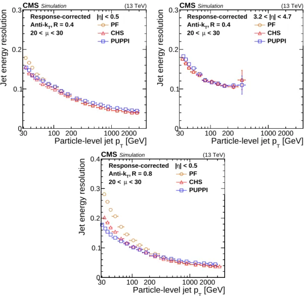
The performance of the jet four-momentum reconstruction is evaluated in QCD multijet simu-lation by comparing the kinematics of jets clustered from reconstructed PF candidates (recon-struction-level jets) to jets clustered from stable (lifetime cτ >1 cm) particles excluding neutri-nos before any detector simulation (particle-level jets). Particle-level jets are clustered without simulation of PU collisions whereas the reconstruction-level jets include simulation of PU col-lisions. Jet energy corrections are applied to the reconstruction-level jets such that the ratio of reconstruction and particle-level jet pT (the response) is on average 1. The jet energy resolu-tion (JER) is defined as the spread of the response distriburesolu-tion, which is Gaussian to a good approximation. The resolution is defined as the σ of a Gaussian fit to the distribution in the range[m−2σ, m+2σ], where m and σ are the mean and width of the Gaussian fit, determined with an iterative procedure. The cutoff at±2σ is set so that the evaluation is not affected by outliers in the tails of the distribution. Figure 3 shows the JER as a function of jet pT for jets reconstructed from all of the PF candidates (PF jets), CHS jets, and PUPPI jets, simulated with on average 20–30 PU interactions. For AK4 jets, the performance of the CHS and PUPPI algo-rithms is similar. Jet resolution for PUPPI is slightly degraded below 30 PU, since PUPPI has been optimized for overall performance, including pmissT resolution and stability, beyond 30 PU interactions. This behavior at low PU can in principle be overcome through a special treatment
in the limit of small amount of PU, where the number of particles to compute αPUand RMSPU
is limited. The PF jets in the detector region of|η| < 0.5 exhibit a worse performance,
particu-larly at low pT, since these jets are more affected by PU. In the region of 3.2< |η| <4.7, PF jets
show the same performance as CHS jets, because no tracking is available. For AK8 jets, PUPPI provides better performance than the CHS and PF algorithms, since neutral particles from PU interactions contribute significantly to such jets.
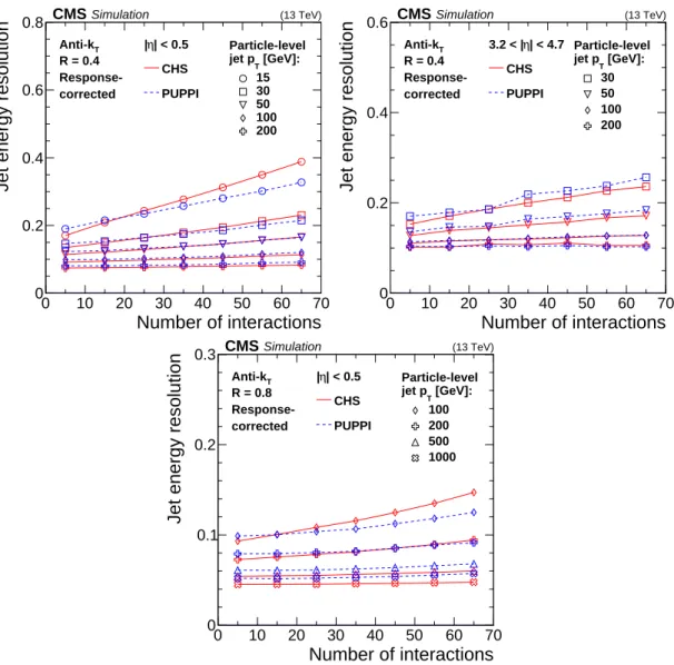
Figure 4 demonstrates how the JER scales with the number of interactions. At more than 30 interactions, JER for AK4 jets with|η| < 0.5 and pT = 30 GeV is better with the PUPPI than
with the CHS PU mitigation. However, JER for AK4 jets with 3.2< |η| <4.7 and pT =30 GeV
is better with the CHS than with the PUPPI PU mitigation, which is a result of the PUPPI algorithm being tuned to yield the best pmissT resolution rather than the best jet resolution in the
|η| >3 region. This is achieved with a low PU particle rate, rather than the best jet resolution,
achieved by high LV particle efficiency. At pT > 100 GeV, PUPPI jets have a resolution that is slightly worse than that of CHS jets with|η| < 0.5, while in 3.2 < |η| < 4.7 PUPPI and CHS
performances are comparable. For AK8 jets at low pT, PUPPI yields a better JER than CHS;
this improvement is present through the high-PU scenarios, e.g., at 50 or 60 interactions. The
jet energy resolution becomes worse with PUPPI than with CHS for jets with pT > 200 GeV.
The behavior of PUPPI at high pT is to a large extent limited by the quality of track-vertex
association using dz for high-pT charged hadrons. The effect is not visible in CHS because
the dz requirement for charged particles that are not associated to any vertex is not used, but instead CHS keeps all charged particles not associated with any vertex.
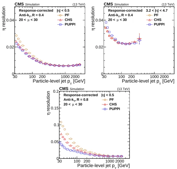
Figure 5 shows the jet η angular resolution simulated with 20–30 interactions. The same quali-tative conclusions also hold for the resolution in φ, since φ and η segmentation of the detector are similar. The resolution is evaluated as the width of a Gaussian function fit to the distribution of the η-difference between the generator- and reconstruction-level jets. The same conclusions as for JER also hold for jet angular resolution. The CHS and PUPPI algorithms perform simi-larly for AK4 jets with|η| <0.5. However, significant improvements from PUPPI are observed
30 100 200 1000 2000 [GeV] T Particle-level jet p 0 0.1 0.2 0.3
Jet energy resolution
(13 TeV) CMSSimulation | < 0.5 η | PF CHS PUPPI , T Anti-k R = 0.4 Response-corrected < 30 µ 20 < 30 100 200 1000 2000 [GeV] T Particle-level jet p 0 0.1 0.2 0.3
Jet energy resolution
(13 TeV) CMSSimulation | < 4.7 η 3.2 < | PF CHS PUPPI , T Anti-k R = 0.4 Response-corrected < 30 µ 20 < 30 100 200 1000 2000 [GeV] T Particle-level jet p 0 0.1 0.2 0.3 0.4
Jet energy resolution
(13 TeV) CMSSimulation | < 0.5 η | PF CHS PUPPI , T Anti-k R = 0.8 Response-corrected < 30 µ 20 <
Figure 3: Jet energy resolution as a function of the particle-level jet pTfor PF jets (orange circles), PF jets with CHS applied (red triangles), and PF jets with PUPPI applied (blue squares) in QCD multijet simulation. The number of interactions is required to be between 20 and 30. The resolution is shown for AK4 jets with |η| < 0.5 (upper left) and 3.2 < |η| < 4.7 (upper
right), as well as for AK8 jets with|η| <0.5 (lower). The error bars correspond to the statistical
5.1 Jet energy and angular resolutions 11 0 10 20 30 40 50 60 70 Number of interactions 0 0.2 0.4 0.6 0.8
Jet energy resolution
[GeV]: T jet p Particle-level 15 30 50 100 200 T Anti-k R = 0.4 Response-corrected | < 0.5 η | CHS PUPPI CMSSimulation (13 TeV) 0 10 20 30 40 50 60 70 Number of interactions 0 0.2 0.4 0.6
Jet energy resolution
[GeV]: T jet p Particle-level 30 50 100 200 T Anti-k R = 0.4 Response-corrected | < 4.7 η 3.2 < | CHS PUPPI CMSSimulation (13 TeV) 0 10 20 30 40 50 60 70 Number of interactions 0 0.1 0.2 0.3
Jet energy resolution
[GeV]: T jet p Particle-level 100 200 500 1000 T Anti-k R = 0.8 Response-corrected | < 0.5 η | CHS PUPPI CMSSimulation (13 TeV)
Figure 4: Jet energy resolution as a function of the number of interactions for jets with CHS (solid red line) and with PUPPI (dashed blue line) algorithms applied in QCD multijet simu-lation for different jet pT values (different markers). The resolution is shown for AK4 jets with
|η| < 0.5 (upper left) and 3.2 < |η| < 4.7 (upper right), as well as for AK8 jets with|η| < 0.5
for AK8 jets for|η| < 0.5. Angular resolution of large-size jets is particularly sensitive to PU
as the clustered energy from PU particles increases with the jet size. Hence, the improvements are larger when PUPPI jets are considered.
30 100 200 1000 2000 [GeV] T Particle-level jet p 0 0.02 0.04 resolution η (13 TeV) CMSSimulation | < 0.5 η | PF CHS PUPPI , T Anti-k R = 0.4 Response-corrected < 30 µ 20 < 30 100 200 1000 2000 [GeV] T Particle-level jet p 0 0.02 0.04 resolution η (13 TeV) CMSSimulation | < 4.7 η 3.2 < | PF CHS PUPPI , T Anti-k R = 0.4 Response-corrected < 30 µ 20 < 30 100 200 1000 2000 [GeV] T Particle-level jet p 0 0.05 0.1 0.15 0.2 resolution η (13 TeV) CMSSimulation | < 0.5 η | PF CHS PUPPI , T Anti-k R = 0.8 Response-corrected < 30 µ 20 <
Figure 5: Jet η resolution as a function of particle-level jet pT for PF jets (orange circles), PF jets with CHS applied (red triangles), and PF jets with PUPPI applied (blue squares) in QCD multijet simulation. The number of interactions is required to be between 20 and 30. The resolution is shown for AK4 jets with|η| < 0.5 (upper left) and 3.2 < |η| < 4.7 (upper right)
as well as for AK8 jets with |η| < 0.5 (lower). The error bars correspond to the statistical
uncertainty in the simulation. 5.2 Noise jet rejection
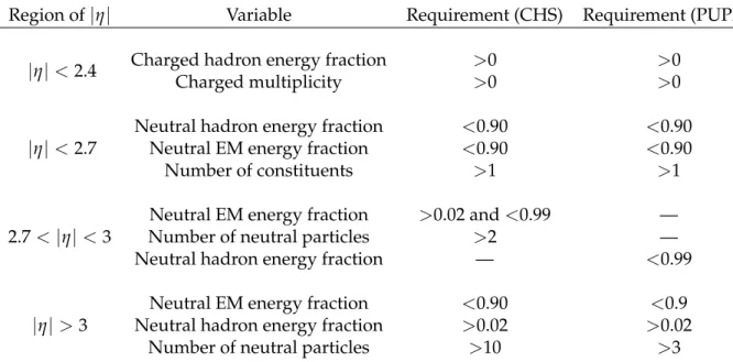
The identification and rejection of jets originating from noise and reconstruction failures are critical to all CMS analyses where a jet or pmissT is used as part of the selection. To further reject noise after detector signal processing and jet clustering, a set of criteria on the PF candidates within a jet are applied [6]. The criteria listed in Table 2 are based on jet constituent energy fractions and multiplicities. They reject residual noise from the HCAL and ECAL, retaining 98– 99% of genuine jets, i.e., jets initiated by genuine particles rather than detector noise. Although PU mitigation algorithms are not designed to have an effect on detector noise, they could, in principle, affect the rejection capability of the noise jet ID.
5.2 Noise jet rejection 13
Table 2: Jet ID criteria for CHS and PUPPI jets yielding a genuine jet efficiency of 99% in differ-ent regions of|η|.
Region of|η| Variable Requirement (CHS) Requirement (PUPPI)
|η| <2.4 Charged hadron energy fraction >0 >0
Charged multiplicity >0 >0
|η| <2.7
Neutral hadron energy fraction <0.90 <0.90
Neutral EM energy fraction <0.90 <0.90
Number of constituents >1 >1
2.7< |η| <3
Neutral EM energy fraction >0.02 and<0.99 —
Number of neutral particles >2 —
Neutral hadron energy fraction — <0.99
|η| >3
Neutral EM energy fraction <0.90 <0.9
Neutral hadron energy fraction >0.02 >0.02
Number of neutral particles >10 >3
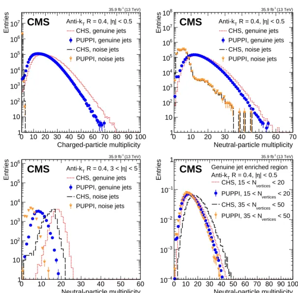
Figure 6 (upper left/right and lower left) shows the distribution of the charged and neutral con-stituent multiplicities comparing genuine jet enriched (dijet) and noise jet enriched (minimum bias) data, demonstrating the separation power. For the dijet selection, data are selected with an HLT requirement of at least one jet having a pT > 400 GeV, two offline reconstructed jets with pTgreater than 60 and 30 GeV, respectively, and an opening in azimuthal angle greater than 2.7. For the minimum bias selection, jets with pT > 30 GeV passing the minimum bias trigger path are used. The noise jet ID requires at least one charged constituent for jets with|η| <2.4 and at
least two constituents (neutral or charged) for|η| < 2.7. The charged constituent multiplicity
is smaller for PUPPI than for CHS jets because PUPPI rejects additional charged particles by
applying a dzrequirement on tracks not associated with any vertex. The PUPPI weighted
neu-tral constituent multiplicity, defined as the sum of PUPPI weights of all neuneu-tral particles in the jet, is also smaller than the neutral constituent multiplicity for CHS. In 3< |η| < 5, the PUPPI
neutral constituent multiplicity is significantly lower than for CHS. Thus, the ability to sepa-rate noise is reduced. With CHS, noise jets are rejected by requiring a minimum of 10 neutral particles. With PUPPI, a minimum of 3 is required for the PUPPI scaled neutral multiplicity. Figure 6 (lower right) demonstrates the PU dependence of the neutral constituent multiplicity. While for CHS, the average multiplicity changes by 30–40% going from 20–30 to 50–60 recon-structed vertices, the PUPPI scaled multiplicities do not change significantly, making noise jet rejection independent of PU.
The efficiency of the jet ID criteria for genuine jets is measured in data using a tag-and-probe procedure in dijet events [6]. The background rejection is estimated using a noise-enriched minimum bias event selection. The fraction of rejected noise jets after applying jet ID crite-ria that yield a 99% efficiency for genuine jets is summarized in Table 3 for different regions in η. The number of noise jets reconstructed with the CHS and PUPPI algorithms is not the same, because the PUPPI reconstruction criteria reject particles that would otherwise give rise to a fraction of noise jets before jet ID criteria are applied. The absolute number of noise jets remaining after PU mitigation and jet ID together differs by less than 20% between CHS and PUPPI jets.
Table 3: Fraction of noise jets rejected when applying jet ID criteria to PUPPI and CHS jets yielding a genuine jet efficiency of 99% in different regions of|η|.
Region of|η| Fraction of noise jets rejected
|η| <2.7 99.9% 2.7 < |η| <3.0 97.6% 3< |η| <5 15% (PUPPI) 35% (CHS) 0 10 20 30 40 50 60 70 80 90 100 Charged-particle multiplicity 1 10 2 10 3 10 4 10 5 10 6 10 7 10 Entries | < 0.5 η R = 0.4, | T Anti-k CHS, genuine jets PUPPI, genuine jets CHS, noise jets PUPPI, noise jets
(13 TeV) -1 35.9 fb
CMS
0 10 20 30 40 50 60 70 Neutral-particle multiplicity 1 10 2 10 3 10 4 10 5 10 6 10 7 10 8 10 Entries | < 0.5 η R = 0.4, | T Anti-k CHS, genuine jets PUPPI, genuine jets CHS, noise jets PUPPI, noise jets(13 TeV) -1 35.9 fb
CMS
0 10 20 30 40 50 60 Neutral-particle multiplicity 1 10 2 10 3 10 4 10 5 10 6 10 Entries | < 5 η R = 0.4, 3 < | T Anti-k CHS, genuine jets PUPPI, genuine jets CHS, noise jets PUPPI, noise jets(13 TeV) -1 35.9 fb
CMS
0 10 20 30 40 50 60 70 80 90 100 Neutral-particle multiplicity 4 − 10 3 − 10 2 − 10 1 − 10 1 Entries Anti-kT R = 0.4, |η| < 0.5Genuine jet enriched region < 20 vertices CHS, 15 < N < 20 vertices PUPPI, 15 < N < 50 vertices CHS, 35 < N < 50 vertices PUPPI, 35 < N (13 TeV) -1 35.9 fb
CMS
Figure 6: The charged- and neutral-particle multiplicities for CHS and PUPPI in a dijet (genuine jets) and minimum bias (noise jets) selection in data. The multiplicities are shown for AK4 jets using CHS reconstructed real jets (red dashed), CHS reconstructed noise jets (black long dashed), PUPPI reconstructed genuine jets (blue circles), and PUPPI reconstructed noise jets (orange triangles). The upper plots show the charged (left) and neutral particle multiplicities (right) for jets with|η| <0.5. The lower left plot shows the neutral particle multiplicity for jets
with 3< |η| < 5. The lower right plot shows the neutral particle multiplicity of AK4 jets with
|η| < 0.5 in a dijet selection in data using CHS and PUPPI for 15–20 and 35–50 interactions.
5.3 Pileup jet rejection 15
5.3 Pileup jet rejection
Particles resulting from PU collisions will introduce additional jets that do not originate from the LV. These jets are referred to as PU jets. PU jets can be classified in two categories: QCD-like PU jets, originating from PU particles from a single PU vertex, and stochastic PU jets, originat-ing from PU particles from multiple different PU vertices. Both PU mitigation techniques,
PUPPI and CHS, remove the charged tracks associated with PU vertices, reducing the pT of
QCD-like PU jets to roughly 1/3 of their original pT, such that they can be largely reduced by selections on the jet pT. In CMS, a multivariate technique to reject the remaining PU jets (dom-inated by stochastic PU jets) has been developed and applied for CHS jets [6], whereas PUPPI intrinsically suppresses PU jets better by rejecting more charged and neutral particles from PU vertices before jet clustering. Both techniques suppress both QCD-like and stochastic PU jets, though the observables used for neutral particle rejection are primarily sensitive to stochastic PU jets.
The performance of the PU jet rejection for both PUPPI and CHS is evaluated in Z+jets events in data and simulation. The jet recoiling against the Z boson provides a pure sample of LV jets, whereas additional jets are often from PU collisions. The Z+jets events are selected by requiring
two oppositely charged muons with pT > 20 GeV and |η| < 2.4 whose combined invariant
mass is between 70 and 110 GeV. Jets that overlap with leptons within ∆R(lepton, jet) < 0.4 from the Z boson decay are removed from the collections of particle- and reconstruction-level jets.
In simulation jets are categorized into four groups based on the separation from particle-level jets and their constituents. If a reconstruction-level jet has a particle-level jet within∆R<0.4, it is regarded as originating from the LV. Jet flavors are defined by associating generated particles to reconstructed jets. This is done by clustering a new jet with the generated and reconstructed particles together where, in this case, the four-momenta of generated particles are scaled by a very small number. Newly reconstructed jets in this way are almost identical to the original jets because the added particles, with extremely small energy, do not affect the jet reconstruction. If a jet originating from the LV contains generated quarks or gluons, it is regarded as a jet of quark or gluon origin, depending on the label of the highest pT particle-level particle. If a jet not originating from the LV does not contain any generated particles from the hard scattering, it is regarded as a jet originating from a PU vertex, i.e., a PU jet. The remaining jets, which do not have nearby particle-level jets but contain particle-level particles (from LV), are labeled as unassigned.
This identification of PU jets is based on two observations: (i) the majority of tracks associated with PU jets do not come from the LV, and (ii) PU jets contain particles originating from mul-tiple PU collisions and therefore tend to be more broad and diffuse than jets originating from one single quark or gluon. Table 4 summarizes the input variables for a multivariate analy-sis. Track-based variables include the LV∑ pTfraction and Nvertices, where the LV∑ pTfraction
is the summed pT of all charged PF candidates in the jet originating from the LV, divided by
the summed pT of all charged candidates in the jet. The LV∑ pT fraction variable provides
the strongest discrimination of any variable included in the discriminator, but is available only within the tracking volume. The inclusion of the Nverticesvariable allows the multivariate anal-ysis to determine the optimal discriminating variables as the PU is increased. Jet shape vari-ables included in the multivariate discriminant are as follows:h∆R2i, f
ring0, fring1, fring2, fring3,
pleadT /pjetT , |~m|, Ntotal, Ncharged, major axis (σ1), minor axis (σ2), and pDT, with their definitions given in Table 4. Pileup jets tend to haveh∆R2iof large value relative to genuine jets. For the
Table 4: List of variables used in the PU jet ID for CHS jets. Input variable Definition LV∑ pT fraction
Fraction of pT of charged particles associated with the
LV, defined as ∑i∈LVpT, i/∑ipT, i where i iterates over all
charged PF particles in the jet Nvertices Number of vertices in the event
h∆R2i Square distance from the jet axis scaled by p2
Taverage of jet
constituents:∑i∆R2p2T, i/∑ip2T, i fringX, X =
1, 2, 3, and 4
Fraction of pTof the constituents (∑ pT, i/pjetT ) in the region Ri < ∆R< Ri+1around the jet axis, where Ri = 0, 0.1, 0.2,
and 0.3 for X=1, 2, 3, and 4
pleadT /pjetT pTfraction carried by the leading PF candidate
pl. ch.T /pjetT pTfraction carried by the leading charged PF candidate
|~m| Pull magnitude, defined as |(∑i pi
T|ri|~ri)|/pjetT where ~ri is
the direction of the particle i from the direction of the jet
Ntotal Number of PF candidates
Ncharged Number of charged PF candidates
σ1 Major axis of the jet ellipsoid in the η-φ space
σ2 Minor axis of the jet ellipsoid in the η-φ space
pD
T Jet fragmentation distribution, defined as
q
5.3 Pileup jet rejection 17
characteristic of PU jets having a large fraction of energy deposited in the outer annulus. Most of the other variables are included to distinguish quark jets from gluon jets, and thus enhance the separation from PU jets. In particular, the variable pDT tends to be larger for quark jets than for gluon jets, and smaller than both quark jets and gluon jets for PU jets. The Ntotal, pD
T and σ2
variables have previously been used for a dedicated quark- and gluon-separation technique; more details on their definition and performance are found in Ref. [6].
Figure 7 shows the distribution of the LV∑ pT fraction and the charged-particle multiplicity
of jets with 30 < pT < 50 GeV and |η| < 1 in data and simulation. The distributions of the
variables in selected data events agree with simulation within the uncertainties, with a clear separation in the discriminating variables between LV and PU jets.
fraction T p ∑ LV 4 − 10 3 − 10 2 − 10 1 − 10 1 10 2 10 3 10
a.u.
Data Quark Gluon Pileup Unassigned Herwig < 50 GeV T 30 < p | < 1 η CHS, |CMS
(13 TeV) -1 35.9 fb , R = 0.4 T Anti-k , R = 0.4T Anti-k 0 0.1 0.2 0.3 0.4 0.5 0.6 0.7 0.8 0.9 1 fraction T p∑
LV 0 1 2 Simulation DataPU uncertainty Herwig/Pythia ⊕ PU uncertainty Charged-particle multiplicity 0.05 0.1 0.15 0.2 0.25
a.u.
Data Quark Gluon Pileup Unassigned Herwig < 50 GeV T 30 < p | < 1 η CHS, |CMS
(13 TeV) -1 35.9 fb , R = 0.4 T Anti-k , R = 0.4T Anti-k 0 2 4 6 8 10 12 14 16 18 20 Charged-particle multiplicity 0 1 2 Simulation DataPU uncertainty Herwig/Pythia ⊕ PU uncertainty
Figure 7: Data-to-simulation comparison for two input variables to the PU jet ID calculation for CHS jets with 30 < pT < 50 GeV: the LV∑ pT fraction (left) and charged-particle multi-plicity (right). Black markers represent the data while the colored areas are Z+jets simulation events. The simulation sample is split into jets originating from quarks (red), gluons (purple), PU (green), and jets that could not be assigned (gray). The distributions are normalized to
unity. The shape of a sample showered with HERWIG++ is superimposed. The lower panels
show the data-to-simulation ratio along with a gray band corresponding to the one-sided un-certainty, which is the difference between simulated Z+jets events showered with the PYTHIA parton shower and those showered with the HERWIG++ parton shower. Also included in the ratio panel is the PU rate uncertainty (dark gray).
The set of 15 variables listed in Table 4 is used to train a boosted decision tree (BDT)
algo-rithm, and to distinguish between jets from the LV and PU jets. For the BDT training, MAD
-GRAPH5 aMC@NLOZ+jets simulation events are used. To perform the training,
reconstruction-level jets that are within a distance of∆R< 0.4 from any particle-level jet are regarded as jets from the LV, and the remaining jets are identified as PU jets. A jet is considered to satisfy the PU jet ID if it passes certain thresholds on the output of the BDT discriminator. This output
is dependent on the η and pT of the jet. Three working points are considered in the following
resulting in different efficiencies and misidentification rates. These working points are defined by their average efficiency on quark-initiated jets. The definitions are:
• tight working point: 80% efficient for quark jets,
• loose working point: 99% efficient for quark jets in|η| <2.5, 95% efficient for quark
jets in|η| >2.5.
Since 92% of the PU jets tend to occur at pT < 50 GeV, the contamination from PU jets with
pT >50 GeV is small. Thus, the PU jet ID is designed to act only on jets with pT <50 GeV. The fraction of PU jets in simulation passing this kinematic event selection is 10% for|η| <2.5,
48% for 2.50< |η| <2.75, 59% for 2.75< |η| <3.00, and 65% for 3< |η| <5. The distribution
of the output BDT discriminator in selected data events and simulation is shown in Fig. 8. Some disagreement is present between the data and simulation. This disagreement is largest
for|η| >2.5 and at low discrimination values, where PU jets dominate. The difference between
data and simulation is roughly comparable to the total uncertainty in simulation, considering
the uncertainty in the number of interactions and the difference to an alternativeHERWIG
++-based parton shower prediction.
BDT output 4 − 10 3 − 10 2 − 10 1 − 10 1 10 2 10
a.u.
Data Quark Gluon Pileup Unassigned Herwig < 50 GeV T 30 < p | < 2.5 η CHS, |CMS
(13 TeV) -1 35.9 fb , R = 0.4 T Anti-k , R = 0.4T Anti-k 1 − −0.8−0.6−0.4−0.2 0 0.2 0.4 0.6 0.8 1 BDT output 0 1 2 Simulation DataPU uncertainty Herwig/Pythia ⊕ PU uncertainty BDT output
4 − 10 3 − 10 2 − 10 1 − 10 1 10 2 10
a.u.
Data Quark Gluon Pileup Unassigned Herwig < 50 GeV T 30 < p | < 5 η CHS, 3 < |CMS
(13 TeV) -1 35.9 fb , R = 0.4 T Anti-k , R = 0.4T Anti-k 1 − −0.8−0.6−0.4−0.2 0 0.2 0.4 0.6 0.8 1 BDT output 0 2 Simulation DataPU uncertainty Herwig/Pythia ⊕ PU uncertainty
Figure 8: Data-to-simulation comparison of the PU jet ID boosted decision tree (BDT) output for AK4 CHS jets with 30 < pT < 50 GeV for the detector region within the tracker volume (left) and 3 < |η| < 5 (right). Black markers represent the data while the colored areas are
Z+jets simulation events. The simulation sample is split into jets originating from quarks (red), gluons (purple), PU (green), and jets that could not be assigned (gray). The distributions are
normalized to unity. The shape of a sample showered with HERWIG++ is superimposed The
lower panels show the data-to-simulation ratio along with a gray band corresponding to the one-sided uncertainty that is the difference between simulated Z+jets events showered with the PYTHIA parton shower to those showered with the HERWIG++ parton shower. Also included in the ratio panel is the PU rate uncertainty (dark gray).
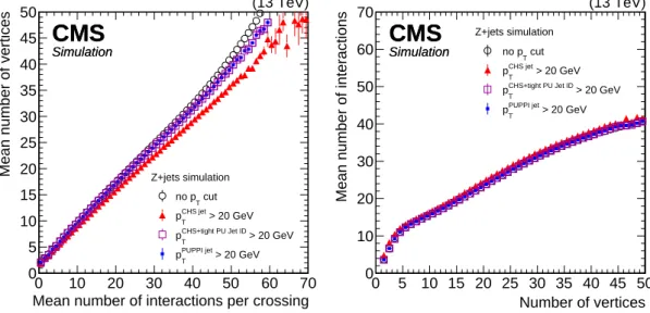
When studying jet performance with PU, it is clear that jet reconstruction and selection, includ-ing PU mitigation, affect the relationship between the number of reconstructed vertices and the mean number of interactions per crossing. The mean number of vertices as a function of the number of interactions can be seen in Fig. 9 (left). Without jet selection, the number of vertices is on average 30% smaller [8, 34] than the number of interactions, because the vertex reconstruc-tion and identificareconstruc-tion efficiency is about 70% (although it is nearly 100% for hard-scattering
interactions). When introducing a selection on the jet pT, the mean number of vertices for a
given number of interactions is reduced. This effect is largest for CHS jets, where no treatment of jets composed of mostly PU particles is present. If a PU vertex is close to or overlaps with the
5.3 Pileup jet rejection 19
LV, jets composed of PU particles end up in the event reconstruction and cause the observed bias. When applying a technique to reduce the number of additional jets composed of mostly PU particles (PUPPI or CHS+tight PU jet ID), the relationship shows a behavior more similar to the one without selection. The mean number of interactions as a function of the number of vertices is presented in Fig. 9 (right). This relationship depends on the assumed distribution of pileup interactions in data and is adjusted to match the 2016 data taking. The largest difference
between events with and without a pTcut is observed for a high number of vertices, while the
different PU mitigation techniques show a similar behavior.
0 10 20 30 40 50 60 70
Mean number of interactions per crossing 0 5 10 15 20 25 30 35 40 45 50
Mean number of vertices Z+jets simulation cut T no p > 20 GeV CHS jet T p > 20 GeV CHS+tight PU Jet ID T p > 20 GeV PUPPI jet T p
CMS
SimulationCMS
Simulation (13 TeV) Number of vertices 0 5 10 15 20 25 30 35 40 45 50Mean number of interactions
0 10 20 30 40 50 60 70 Z+jets simulation cut T no p > 20 GeV CHS jet T p > 20 GeV CHS+tight PU Jet ID T p > 20 GeV PUPPI jet T p
CMS
SimulationCMS
Simulation (13 TeV)Figure 9: Left: distribution of mean number of reconstructed vertices as a function of the mean number of interactions in Z+jets simulation. Right: distribution of the mean number of interac-tions as a function of the number of vertices in Z+jets simulation. The black open circles show the behavior without applying any event selection, while for the other markers a selection on jets of pT > 20 GeV is applied using the CHS (full red triangles), CHS+tight PU jet ID (vio-let open squares), and PUPPI (full blue squares) algorithms. The error bars correspond to the statistical uncertainty in the simulation.
Figure 10 shows the LV jet efficiency and purity in Z+jets simulation as a function of the num-ber of interactions for CHS jets, CHS jets with a PU jet ID applied, and PUPPI jets. The ef-ficiency is defined as the fraction of particle-level jets with pT > 30 GeV that match within ∆R<0.4 with a reconstruction-level jet with pT >20 GeV. The purity is defined as the fraction of reconstruction-level jets with pT > 30 GeV that match within∆R< 0.4 with a particle-level jet with pT > 20 GeV from the main interaction. The pT cuts at reconstruction and generator level are chosen to be different to remove any significant JER effects on this measurement. For CHS jets, the efficiency is larger than 95% in entire detector region up to |η| < 5
regard-less of the number of interactions. However, the purity drops strongly with the number of interactions down to 70 and 18% at 50 interactions for the regions of|η| < 2.5 and|η| > 2.5,
respectively. The PU jet ID applied on top of CHS reduces the efficiency with respect to using only CHS, but at the same time improves the purity, especially for low-pTjets. In|η| <2.5, the
loose working point has only a slightly reduced efficiency compared to CHS alone. In|η| >2.5,
the efficiency drops to roughly 80% at high PU for the loose working point. In|η| < 2.5, the
purity remains constant at around 98% over the whole range of PU scenarios. In|η| > 2.5, the
purity is PU-dependent, but improves over CHS alone by a factor of 1.7 at high PU for the loose working point. The tight PU jet ID achieves the best purity in|η| >2.5 at 40% with collisions
CHS by removing neutral particles. At the same time, PUPPI improves the purity by removing PU jets from the event without the need of a PU jet ID. At low PU (below 10 interactions), the purity of PUPPI jets is equal to that of CHS. At high PU, the purity of PUPPI jets with respect to CHS jets is significantly higher than that of CHS jets. PUPPI has a constant efficiency above 95% in|η| < 2.5, and a purity compatible with the tight PU jet ID working point at high PU.
In |η| > 2.5, above 30 interactions the efficiency of PUPPI is better than the loose PU jet ID,
whereas the purity is compatible to within a few percent to the loose PU jet ID. In summary, PUPPI shows an intrinsic good balance between efficiency and purity compared to CHS, but if purity in|η| > 2.5 is crucial to an analysis, CHS+tight PU jet ID yields better performance.
Using variables designed to distinguish quark jets from gluon jets results in a<1% difference for 20 < PU < 30 in efficiency for PUPPI and CHS in |η| <2.5 and range up to 5% (12%) in |η| >3 for PUPPI (CHS) with tight PU ID.
To evaluate the performance of PU jet identification in data, the ratio of PU jets to genuine jets for the leading pT jet in the event is studied. Events are split into two categories to compare both PU and LV jets. The categorization is performed utilizing the difference between the
az-imuths φ of the leading pT jet and the Z boson. The PU-enriched events are required to have
∆φ(Z boson, jet) <1.5, while events enriched in LV jets are required to have∆φ(Z boson, jet) >
2.5. Figure 11 shows the rate of events in the PU-enriched region divided by the rate of events in the LV-enriched region, as a function of the number of vertices for CHS jets, CHS jets with medium PU jet ID applied, and PUPPI jets in Z+jets simulation and data. The rate of PU-enriched events selecting CHS jets alone exhibits a strong dependence on the number of ver-tices in detector regions where|η| <2.5. This dependence increases from 8 to 25% when going
from 5 to 40 vertices. The dependence is strongly reduced when the PU jet ID is applied or PUPPI is utilized. PUPPI shows a stable behavior across the whole range in|η| <2.5 for both
data and simulation. For|η| >2.5, all three algorithms show a PU dependence with CHS jets
having the worst performance. Furthermore, categorization with PUPPI jets has a PU-enriched rate between that of events categorized with CHS and CHS+medium PU jet ID. For reference, the rate of jets that are matched to a particle-level jet in simulation is also shown for CHS jets (simulation, CHS LV). This line shows the expected ratio of events in the two regions when only the LV jets are used for the categorization. This curve shows a slight PU dependence because of the high matching parameter of generator- with reconstruction-level jets (∆R<0.4).
Scale factors for the efficiency of data and simulation for both matched jets from the LV and PU jets for various PU jet ID working points are derived using the event categories enriched in genuine jets and PU jets. Scale factors are within a few percent of unity in the detector region where|η| <2.5. In|η| >2.5, they are farther from unity, with differences up to 10% for jets with
2.5< |η| <3.0 and the tight working point applied. The scale factor for PU jets is significantly
larger and leads to a visible disagreement in Fig. 11. This disagreement is found to be as large as 30% for low pTjets with|η| >2.5. The difference in modeling when usingHERWIG++ instead of
PYTHIAfor parton showering shown in the lower panel of Fig. 11 is considered as an additional
uncertainty. The difference of data with respect toPYTHIA showered jets is contained within
the total variation when considering bothHERWIG++ andPYTHIAbased parton showers.
6
W, Z, Higgs boson, and top quark identification
6.1 Jet substructure reconstruction
In various searches for new physics phenomena and measurements of standard model prop-erties, top quarks, W, Z, and Higgs bosons are important probes. They can be produced
6.1 Jet substructure reconstruction 21 Number of interactions 0 20 40 60 Efficiency 0.65 0.7 0.75 0.8 0.85 0.9 0.95 1 1.05 1.1 CHS CHS + tight PU jet ID CHS + medium PU jet ID CHS + loose PU jet ID PUPPI Number of interactions 0 10 20 30 40 50 60 70
CMS
SimulationCMS
Simulation (13 TeV) > 20 GeV reco T > 30 GeV, p gen T p | < 2.5 η , R = 0.4, | T Anti-kT, R = 0.4, |η| < 2.5 Anti-k > 20 GeV reco T > 30 GeV, p gen T p Number of interactions 0 20 40 60 Efficiency 0 0.2 0.4 0.6 0.8 1 1.2 CHS CHS + tight PU jet ID CHS + medium PU jet ID CHS + loose PU jet ID PUPPI Number of interactions 0 10 20 30 40 50 60 70CMS
SimulationCMS
Simulation (13 TeV) > 20 GeV reco T > 30 GeV, p gen T p | < 5 η , R = 0.4, 3 < | T Anti-kT, R = 0.4, 3 < |η| < 5 Anti-k > 20 GeV reco T > 30 GeV, p gen T p Number of interactions 0 20 40 60 Purity 0.5 0.6 0.7 0.8 0.9 1 1.1 1.2 CHS CHS + tight PU jet ID CHS + medium PU jet ID CHS + loose PU jet ID PUPPI Number of interactions 0 10 20 30 40 50 60 70CMS
SimulationCMS
Simulation (13 TeV) > 30 GeV reco T > 20 GeV, p gen T p | < 2.5 η , R = 0.4, | T Anti-kT, R = 0.4, |η| < 2.5 Anti-k > 30 GeV reco T > 20 GeV, p gen T p Number of interactions 0 20 40 60 Purity 0 0.1 0.2 0.3 0.4 0.5 0.6 0.7 0.8 0.9 CHS CHS + tight PU jet ID CHS + medium PU jet ID CHS + loose PU jet ID PUPPI Number of interactions 0 10 20 30 40 50 60 70CMS
SimulationCMS
Simulation (13 TeV) > 30 GeV reco T > 20 GeV, p gen T p | < 5 η , R = 0.4, 3 < | T Anti-kT, R = 0.4, 3 < |η| < 5 Anti-k > 30 GeV reco T > 20 GeV, p gen T pFigure 10: The LV jet efficiency (upper) and purity (lower) in Z+jets simulation as a func-tion of the number of interacfunc-tions for PUPPI (blue closed squares), CHS (red closed triangles), CHS+tight PU jet ID (magenta open squares), CHS+medium PU jet ID (orange crosses), and CHS+loose PU jet ID (black triangles). Plots are shown for AK4 jets pT > 20 GeV, and (left)
|η| < 2.5 and (right) |η| > 3. The LV jet efficiency is defined as the number of matched
reconstruction-level jets with pT > 20 GeV divided by the number of particle-level jets with pT >30 GeV that originate from the main interaction. For the lower plots, the purity is defined as the number of matched particle-level jets with pT >20 GeV divided by the number of recon-structed jets that have pT > 30 GeV. The error bars correspond to the statistical uncertainty in the simulation.