Comparison of ARIMA and RBFN models to predict the bank transactions

Information Technology Jownal 6 (3): 475-477, 2007 ISSN 1812-5638

© 2007 Asİan Network for Scientific Information

Comparison of ARIMA and RBFN Models to Predict the Bank Transactions Mitat Uysal

Department of Computer Engineering, Dogus University, Acıbadem, Kadikoy, Istanbul, Turkey

Abstract: In this research, Radial Basİs Fwıction Networks (REFN) and ARIJ\1A models(Autoregressive Integrated Moving Average) are compared to theİr ability to predict time series values. RBFN gives good results İn many cases but for some extreme values of time series, better approximatiollS can be obtained using ARIJ\1A models.

Key words: Time series prediction, radial basİs flUletion networks, ARIJ\1A models, simulation, neuraI networks, fwıction approximation

DESC RIPTION OF THE P ROBLEM

In real world applications, many processes can be represented using time series models as below:

x(t - P ), ... x(t - 2),x(t - l),x(t)

F or making a prediction using time series, a large variety of approaches are available. Prediction of scalar time-series {x(n)} refers to the task of finding an estimate x(n+ 1) of the next future sample x(n+l ) based on the knowledge of the history of time-series, i,e., the samples x(n), x(n-l ), ... (Rank,2003).

Linear prediction, where the estimate is based on a linear combination of N past samples can be represented as below:

N-ı

x(n+l)� 2: O:ix(n-i) i=O

with the prediction coefficients (x" i = 0,1, ... N-I.

Introducing a general nonlinear fwıction f(·); mn .... m apphed to tbe vector x(n) � [x(n), x(n - M), ... , x(n-(N­ l»M]T of past samples, we arrive at the nonlinear prediction approach x(n + I) � f(x(n» (Rank, 2003).

ARIMAMODEL

Traditionally, time series forecasting problem is tackled using linear techniques such as Auto Regressive Moving Average (.ARlv1A) and Auto Regressive Integrated Moving Average (ARIMA) models popularized by Box and Jenkins (1976).

475

The general form of ARMA(p,q) model can be written as below:

p q

Xt - L �Xt-r = L 8sGt-s

r=1 s=O

where {E\} is white noise. This process is stationary for appropriate <1>, e (Box and Tenkins, 1976).

The general form of the ARI1.1A model is given by:

i � 1,2, ... p and j � O, 1, ... Q where Yı is a stationary stochastic process with non-zero mean, ao is the constant coefficient, e! the white noise disturbance term, a, represents autoregressive coefficients and bJ denotes the moving average coefficients.

RA DIAL BASIS FUNCTION NETWORK

The RBF network consists of 3 layers: an input layer, a hidden layer and an output layer. A typical RBF network is shown in Fig. 1.

Mathematically, the network output for linear output nodes can be expressed as below:

Where x is the input vector with elements Xi (where i

is the dimension of the input vector); ;ZJ is the vector to determine _ the center of the basis fwıction; <L>J with elements xJ! ; Wlg 's are the weights and Wko is the bias (Duy and Cong, 2003). The basis function <1>,(-) provides the non-linearity.

Inform. TechnoZ. J .• 6 (3): 475-477. 2007

x,

x, _yk(x)

X.

Fig. 1: Typical RBF network

BASIS FUNCTIONS

y"

y�

y�

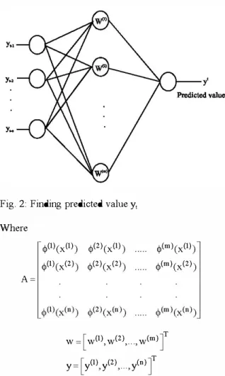
Fig. 2: Finding predicted value Yı Where

�(1)(x(1» �(2)(x(1»

�(1)(x(2) �(2)(x(2)

�(m)(x(2»

�(m)(x(1»

y'

The most used basİs [wıctiorn are Gaussİan and _A = multiquadratic [wıctions. They are given below:

• Gaussİan

<I>(x) � exp(-x'/2ö') for ö > O and x E »!

• Multiquadratic <I>(x) � (x'+ö')' for ö > O and XE»! p is between O and 1. Usually p İs taken as IIz.

CALCVLATING THE OPTIMAL VALUES OF WEIGHTS

A very important property of the RBF Network is that it İs a linearly weighted network İn the sense that the üutput İs a linear combination of ın radial basİs [wıCtiOllS,

wrİtten as below:

f(x)

�

�

(

)�

(

)

The main problem İs to [ind the urıknoWIl weights (i) ın

(w ı.�1

F or this purpose, the general least squares principal can be used to minimize the surn squared error:

SSE�.:1: [y(i)_f(x(i»]2

= ı

With respect to the weights of f, resulting in a set of

ın sİmultaneous ıınear algebraic equatiollS İn the ın

unknown weights (NA) w � A 'y

476

w�[ w(1),w(2), ... ,w(m)r

y� [y<1),y<2)

r

In the special case where II = ID, the resultant system

is just Aw � Y (Duy and Cong, 2003).

The output y(x) represents the next value of Y in time t taking input values xi> x2> ... , � that represent the previous flUlction values set with values Yı.ı> Yı.;; ... , Y ı.n So, xn corresponds to Yı.ı> xn.ı corresponds to Yı.2 etc. as in Fig. 2.

SIMVLA TION RESVL TS

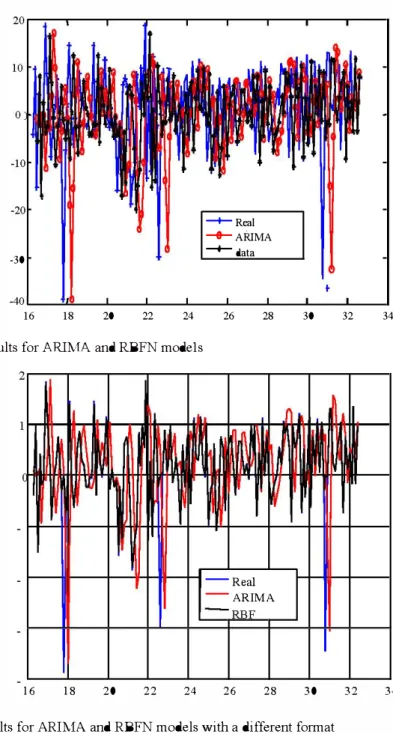
F or this work, the time series data of American Express Bank is used. Monthly log data consists of 324 data items. The first 162 data items are used for training and the remaining 162 data items are used for forecasting. Figure 3 shows the results of simulation nın with

o = 1.5 and 18 neurons in the hidden layer of the Radial

Basis FlUlction Network with the results of ARI1.1A model for the same data.

As in Fig. 3 and 4, RBFN approach provides better results than ARI1.1A model in a big part of data interval except the peak points.

In this points, ARI1.1A model gives better results than RBFN approach.

Inform. Techno/. J .• 6 (3): 475-477. 2007 20��.---'---<r--�---,----r---�---r---, --+-Rea! -+-ARTMA -30 -+- data -40� __ � __ -L __ � ____ � __ -L __ �� __ ı-__ -L __ � 16 18 20 22 24 26 28 30 32 34

Fig. 3: Simulation Results for ARIMA and RBFN mode1s

2r-�.---,----r---.---,r---.---,----r---,

--Rea!

-ARIMA

16 18 20 22 24 26 28 30 32 34

Fig. 4: Simulation results for ARI1.1A and RBFN models with a different format

CONCLUSIONS

Radial Basİs Fwıctions N etworks provide a good way to predict the future values ın a time senes. In the peak points of the original data, ARI1.1A model gives better results than RBFN approach.

In order to obtaİn the best results of the whole İnterval of the data, a hybrid model that consİsts of ARI1.1A and RBFN approach can be used to predict the future values of the time series.

477

REFERENCES

Box. G.E.P. and G.M. Jenkins. 1976. Time Series Ana1ysis: Forecasting and Control. Holden Day Ine. San Francisco, CA.

Duy. N.M.. and T.T. Cong. 2003. Approximation of fwıction and its derivations using radial basİs flUletion networks. Applied Mathematical Modelling, 27: 197-220.

Rank. E.. 2003. Application of Bayesian trained RBF networks to nonlinear time-series modeling. Signal Processing. 83: 1393-1410.