Effect of different network geometry on GNSS results

T.R.

SELÇUK UNIVERSITY

THE GRADUATE SCHOOL OF NATURAL AND APPLIED SCIENCE

EFFECT OF DIFFERENT NETWORK GEOMETRY ON GNSS RESULTS

Shamal Fatah Ahmed AHMED MASTER THESIS

Department of Geomatics Engineering

December-2017 KONYA All Rights Reserved

iv

ABSTRACT

MS THESIS

EFFECT OF DIFFERENT NETWORK GEOMETRY ON GNSS RESULTS Shamal Fatah Ahmed AHMED

THE GRADUATE SCHOOL OF NATURAL AND APPLIED SCIENCE OF SELCUK UNIVERSITY

THE DEGREE OF MASTER IN GEOMATICS ENGINEERING

Advisor: Assoc. Prof. Dr. Ramazan Alpay ABBAK 2017, 46 Pages

Jury

Assoc. Prof. Dr. Ekrem TUŞAT Assoc. Prof. Dr. Ramazan Alpay ABBAK

Assist. Prof. Dr. Serkan DOĞANALP

Global Navigation Satellite System (GNSS) is mostly used to establish geodetic networks in surveying engineering. To establish a geodetic network, one should have an understanding of the various types of geodetic networks, their design, accuracy requirements, and essence. The main area where GNSS networks are needed include mapping, tracking crustal movements, planning large engineering projects, implementing cadastral works, designing urbanization activities, GIS, etc. In GNSS network, stations are generally located where they are needed, but the observation schema between stations are important.

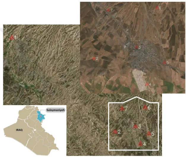
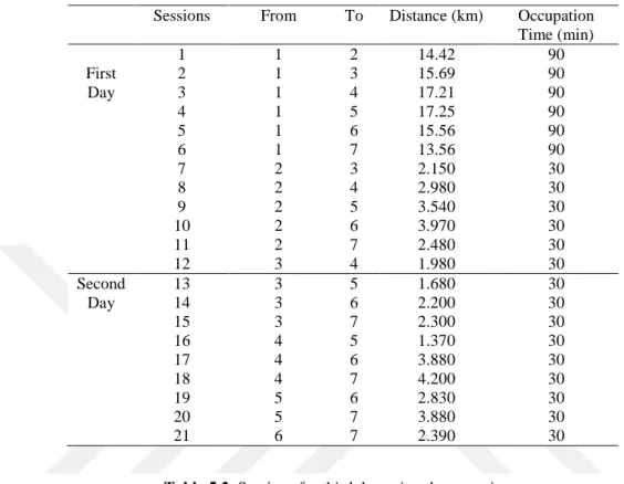
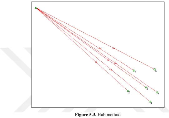
The main goal of this research was to select the best observation schema of GNSS networks according to the number of receivers and the redundancy of the observation. In this research, six points were established after reconnaissance the field of the project. After preparation the sessions according to the number of receivers, time, and distance between points observations were made by using static method. Data collections were made by using two and three receivers. From data collected in three days four types of geometric design of GNSS network were selected. The first was Hub method that is from one fixed point the new points (i.e. six points in this study) were observed. The second one was Star method that is one fixed point in the center of the new network and observed unknown points. The third was Loop method 1 (using two receivers) where all baselines (i.e. 21 baselines in this study) were observed from one known point and the last was Loop method 2 (using three receivers) from one fixed point. These methods had some advantage and disadvantage according to the type of the project that are selected. Due to no redundancy, no close loop, and no nontrivial line between adjacent points the first and second methods are not recommended for the establishment of the precise GNSS network in our study.

v

ÖZET

YÜKSEK LİSANS TEZİ

FARKLI AĞ GEOMETRİSİNİN GNSS SONUÇLARINA ETKİSİ Shamal Fatah Ahmed AHMED

Selçuk Üniversitesi Fen Bilimleri Enstitüsü Harita Mühendisliği Anabilim Dalı Danışman: Doç. Dr. Ramazan Alpay ABBAK

2017, 46 Sayfa Jüri

Doç. Dr. Ekrem TUŞAT Doç. Dr. Ramazan Alpay ABBAK Yrd. Doç. Dr. Serkan DOĞANALP

GNSS (Global Navigation Satellite System) arazi ölçmelerinde jeodezik ağların kurulmasında sıkça kullanılır. Bir jeodezik ağı kurmak için, ağın türünü, tasarımını, doğruluk isteklerini bilmek gerekir. GNSS ağının ihtiyaç olduğu alanlar; haritalama, yer kabuğu hareketlerinin izlenmesi, geniş çaplı mühendislik projelerinin planlanması, kadastral çalışmalarının uygulanması ve CBS aktivitelerini içerir. GNSS ağında, noktalar nerede ihtiyaç duyulursa orada tesis edilir. Fakat noktalar arasındaki gözlem şeması önemlidir.

Bu çalışmanın ana amacı; fazla gözlem sayısı ve alıcı sayısı düşünülerek GNSS ağında en uygun ölçü tasarımını belirlemektir. Bu kapsamda proje sahasında 6 nokta tesis edilmiştir. Oturumlar hazırlandıktan sonra, alıcı sayısı, noktalar arası uzaklık ve zaman göz önünde bulundurularak statik ölçüler gerçekleştirilmiştir. 3 günlük veri toplam sürecinde GNSS ağının farklı 4 çeşit ağ tasarımı denenmiştir. Veri toplama sürecinde iki ve üç alıcı kullanılmıştır. Birincisi bir sabit noktadan yeni noktalara ölçü yapan Hub metodudur (yeni nokta sayısı 6 dır). İkincisi ağın merkezindeki bir noktayı sabit alıp diğer noktaları gözlemleyen Star yöntemidir. Üçüncüsü bilinen bir noktadan tüm noktaların gözlemlendiği iki alıcılı Loop yöntemidir. Sonuncusu iki sabit noktalı ve üç alıcılı Loop yöntemidir. Seçilen projelerin türüne göre yöntemlerin üstünlükleri ve zayıflıkları bulunmaktadır. Sayısal sonuçlara göre fazla ölçü sayısındaki eksiklik ve kapalı lupların olmaması nedeniyle birinci ve ikinci yöntem, yüksek duyarlıklı GNSS ağ tasarımında tavsiye edilmez.

vi

ACKNOWLEDGEMENT

All gratitude is to almighty ALLLAH who guided me and granted me the health, strength, the patience and the opportunity to complete my MSc thesis. I would like to thank my Advisor Assoc. Prof. Dr. Ramazan Alpay ABBAK for his supervision, support, and continuous encouragement during the preparation of the thesis.

Also l would like to thank Assoc. Prof. Dr. İsmail ŞANLIOĞLU for his support for post processing my data, and special thanks to Prof. Dr. Cevat İnal and his Assistant. Sercan

BÜLBÜL for their support and advices.

Special thanks to my friend PhD Student Tibebu Belete for his help at the time of writing my thesis. Special thanks to my special family for their incomparable support, motivation, and assurance during all my life.

My thanks also to all those who helped me, in one way or another, to achieve my MSc thesis.

vii

TABLE OF CONTENTS

ABSTRACT ... iv

ÖZET ... v

ACKNOWLEDGEMENT ... vi

TABLE OF CONTENTS ... vii

ABBREVIATIONS ... ix

1. INTRODUCTION ... 1

2. GEODETIC CONTROL NETWORK ... 2

2.1. Types of Geodetic Control ... 2

2.2. Accuracy Standards and Specifications for Control Surveys ... 3

2.3. Network and Local Accuracy Standards ... 5

2.4. Network Design ... 6

2.5. Reconnaissance for Site Selection ... 7

2.6. Monumentation ... 9

2.6.1. Three dimensional monuments ... 10

3. OVERVIEW OF GNSS ... 11

3.1. Global Positioning System (GPS) ... 11

3.1.1. GPS history ... 11

3.1.2. GPS segments ... 11

3.2. GLObal NAvigation Satellite System (GLONASS) ... 14

3.3. Reference Coordinate Systems ... 15

3.4. GNSS Positioning ... 16

3.5. GNSS Error Sources ... 18

3.5.1. Satellite clocks ... 19

3.5.2. Orbit errors ... 19

3.5.3. Ionosphere and tropospheric error ... 19

3.5.4. Multipath error ... 20

3.5.5. Other error sources ... 21

3.6. Satellite Geometry and Dilution of Precision in GNSS ... 21

3.7. GNSS Positioning Modes ... 22

3.8. Field Procedures in GNSS Surveys... 23

3.8.1. Static method ... 23

3.9. Mission Planning ... 25

3.10. Observation Scheme and Redundancy ... 25

4. DATA PROCESSING AND ANALYSIS ... 30

4.1. Network Pre-Adjustment Data Analysis ... 30

4.2. Baseline Network Adjustment ... 30

viii 5. NUMERICAL APPLICATION ... 33 5.1. Study Area ... 33 5.2. GNSS Data ... 33 5.3. Results ... 35 6. CONCLUSION ... 42 REFERENCES ... 43 CURRICULUM VITAE... 46

ix

ABBREVIATIONS

BeiDou : Chinese Navigation Satellite System

C/A code : Coarse/Acquisition Code

CL : Civilian Long

CM : Civilian Moderate

DOP : Dilution of Precision

ECC : Eccentric

FGCS : Federal Geodetic Control Subcommittee

FGDC : Federal Geographic Data Committee

GDOP : Geometric Dilution of Precision

GIS : Geographic Information System

GLONASS : Global Navigation Satellite System

GNSS : Global Navigation Satellite System

GPS : Global Positioning System

HDOP : Horizontal Dilution of Precision

IGEB : Interagency GPS Executive Board

IRNSS : Indian Regional Navigation Satellite System

ISS : Inertial Surveying System

L1C : Fourth Civilian GPS Signal

L2C : Second Civilian Code on the L2 Signal

NAVSTAR : Navigation by Satellite Ranging and Timing

NGA : National Geospatial Intelligence Agency

OCS : Operational Control Segment

P code : Precise Code

PDOP : Position Dilution of Precision

PPP : Precise Point Positioning

PRN : Pseudorandom Noise Code

QZSS : Quasi-Zenith Satellite System

RDOP : Relative Dilution of Precision

RTK : Real Time Kinematic

SA : Selective Availability

SBAS : Spaced Based Augmentation System

TDOP : Time Dilution of Precision

USSR : Union of Soviet Socialist Republics

UTC : Coordinated Universal Time

VDOP : Vertical Dilution of Precision

1. INTRODUCTION

Engineering surveying mainly concerns fixing the position of any point. According to Kuang (1996), geodetic positioning determines the coordinates of a point(s) on land, at sea, or in space in regard to a predefined coordinate system. It is also accomplished by making measurements that link the unknown point(s) to points with known coordinate values that might be either terrestrial points or extraterrestrial objects (stars or satellites, or both). Based on the number of unknown points, geodetic positioning is categorized into point, relative, and network positioning, which is focused on determining the coordinates of one point, the relative location of one point with respect to another, and the relative locations among a group of three or more points. Nowadays, with the evolution of new science and technology, a wide category of disciplines have indicated the need for a network of appropriately distributed points of known horizontal and/or vertical coordinates. Kuang (1996) reported that, the main areas where geodetic control networks are required include mapping, boundary demarcation, urban management, engineering projects, geographic information system (GIS), hydrography, environmental management, ecology, earthquake-hazard assessment, aerial photography, space research, astronomy, geophysics, deformation monitoring, etc. It may be categorized as being of a local, regional, national, or global level.

This research was discussed about four types of GNSS network design [Hub, Star, Loop method 1 (using two receivers) and Loop method 2 (using three receivers)]. Anonymous1 (2014) described two types of GNSS network design theoretically as Hub and Loop method from one fixed point. It also presents the advantages and disadvantages of them. However, this study numerically described the four types and comparison between them based on the standard deviation of coordinates and the position quality of points as well.

This thesis started with the general principle of geodetic networks, their design, accuracy and monuments. Then the overview of GNSS was described, like GPS and GLONASS’s principle and GNSS positioning. Also field procedure using methods like static method, and observation schema and redundancy were described. After that, data processing and analysis was presented. Then in the application chapter, we discussed about project area, methods and comparison between them. Finally, results of this research were summarized in the last section.

2. GEODETIC CONTROL NETWORK

The locations of points of interest are represented by the value of coordinates that are referenced to a predefined mathematical surface (i.e., datum) (Anonymous2, 2002). A datum is a coordinate surface used as reference figure for positioning control points. Control points are defined as relative positions that are connected to each other in the network. According to datum, its coordinates represent the location of any point. The reference surface for a station is defined by its location relative to the size and shape of the Earth. Densification of a control point network means adding control points to the network and extending the scope. Anonymous2 (2002) stated that in surveying and geomatics engineering to reference coordinates of network control points both horizontal and vertical datum commonly are used to launch a geodetic network, one should have an understanding of the various types of geodetic networks, their design, accuracy requirements, and essence (Bundoo, 2013).

2.1. Types of Geodetic Control

According to Torge (1991), there are three basic types of geodetic control: Those are horizontal, vertical and gravity. This research was focused on horizontal control type. Horizontal control is a network of control points of well-known geographic or grid coordinates related to a horizontal datum, the horizontal positions of those controls of mapped features relative to northing and easting grid lines, or latitude and longitude shown on the map (Anonymous3, 1973).

In horizontal control surveys, the field procedures have traditionally been the main techniques of trilateration, precise traversing, triangulation, and combinations. Furthermore, astronomical observations were made to determine azimuths, latitudes, and longitudes.

Inertial Surveying Systems (ISSs) were introduced during the era of 1970s. ISSs were used in a variety of surveying applications, and one of the most important being control surveying. Some of the limitations of these systems were their high initial cost, equipment that was bulky, and an overall accuracy less than that attainable with Global Navigation Satellite System (GNSS) receivers. Because of this, ISSs are no longer used for control surveys. They are used in mobile mapping units since they can carry coordinates in areas where canopy conditions obstruct GNSS satellite signals. Satellite

surveying has been employed with increasing frequency, especially in control surveys. Because of its ease of use, quickness, and very high precision capabilities at long baselines, GNSS surveys are rapidly replacing the other methods. Nevertheless, in small areas, traditional methods of establishing control are still being used (Ghilani and Wolf, 2015).

2.2. Accuracy Standards and Specifications for Control Surveys

The accuracy required for a control survey depends mainly on its purpose. The type and health of the equipment used, the field procedures employed, and the experience and skills of the employed staff are some of the key factors that influence accuracy. In 1984, and 1998, the Federal Geodetic Control Subcommittee (FGCS) has published several sets of detailed accuracy standards and specifications for geodetic surveying. The rationale for both sets of standards is twofold: (1) Providing a set of standards that define the least acceptable accuracy of control surveys for different purposes, and (2) specifications are established for instrumentation, field procedures, and misclosure checks to ensure that the designated level of accuracy is achieved. In 1998, FGCS was stated the different accuracy standards for control points. This standard is free of the survey method and is based on a 95% confidence level. To meet these standards, the control point of the survey should match with all other points of the geodetic control network. For horizontal surveys, the accuracy standard specifies the radius of a circle within which the actual or theoretical position of the survey point is within 95% of the time.

According to the above standards, procedures leading to classification involves four steps (Anonymous1, 2014; Ghilani and Wolf, 2015; Ogundare, 2015): The first step consists of survey observations, field records, sketches, and other documentation. The second step is free adjustment of the survey observations. The third step is the accuracy of control points in the local existing network to which the survey is tied and the fourth step is the survey accuracy, which is checked at the 95% confidence level by comparing free adjustment results on the established control. This comparison takes into account systematic effects such as crustal motion and datum distortion as well as network accuracy of existing controls. This initial set of standards was established three unique accuracy orders to manage traditional control surveys in descending order of first, second,

and third orders. The class I and class II are two separate accuracy classes of second and third orders for horizontal control surveys.

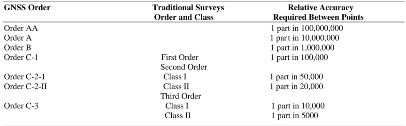
According to research results, three new orders of accuracy were defined for GNSS surveys. These were orders AA, A, and B. Another lower order of accuracy was identified as order C and also specified in these standards. It overlaps the three orders of accuracy applied to traditional horizontal surveys (Table 2.1). Traditional surveys are included horizontal control standards and specifications (Ogaja, 2011; Ghilani and Wolf, 2015).

FGCS accuracy standards required for the various orders and classes of horizontal and vertical control surveys, respectively. In the Table 2.1 values are ratios of allowable relative positional errors of a pair of horizontal control points, to the horizontal distance separating them. Thus, two first-order stations located 100 km apart are expected to be correctly located with respect to each other to within ±1m. The ultimate success of any engineering or mapping project depends on appropriate survey control. The higher order of accuracy is demanded, more time and expense are required. It is therefore important to select the proper order of accuracy for a given project and carefully follow the specifications. Note that no matter how accurately a control survey is conducted, errors will exist in the computed positions of its stations, but a higher order of accuracy presumes smaller errors (Ogaja, 2011; Ghilani and Wolf, 2015).

The primary uses of horizontal control are as follows:

1. GNSS surveyed control points that meet the Order AA and Order A standards are common in global, national, and regional networks that are primarily used for geodynamic and deformation studies.

2. The GNSS survey points that have increased the network density within the areas enclosed by primary control are performed to GNSS Order B standards. These networks are common in high-value land areas and are commonly used for high precision engineering surveys.

3. Survey control to meet mapping, GIS, property surveys, and engineering needs are set by traverse and triangulation to first and second-order stations, and by GNSS to Order C standards.

4. Controls for local construction projects and small terrain mappings are based on high level control monuments and can be set as third order class I or class II standards, depending on the desired accuracy.

Table 2.1. 1984 and 1985 FGCS Horizontal Control Survey Accuracy Standards (Ogaja, 2011; Ghilani

and Wolf, 2015)

GNSS Order Traditional Surveys Relative Accuracy Order and Class Required Between Points

Order AA 1 part in 100,000,000 Order A 1 par t in 10,000,000 Order B 1 part in 1,000,000 Order C-1 First Order 1 part in 100,000 Second Order

Order C-2-1 Class I 1 part in 50,000 Order C-2-II Class II 1 part in 20,000 Third Order

Order C-3 Class I 1 part in 10,000 Class II 1 part in 5000

2.3. Network and Local Accuracy Standards

There are two types of accuracy classification in the Federal Geographic Data Committee (FGDC) publications, which are network accuracy and local accuracy. Network accuracy is aimed at measuring the contact between the control point in question and the realization of datum. Besides, local accuracy measures location accuracy for different points in the same network (Ogaja, 2011; Anonymous1, 2014; Anonymous4, 2015; Ogundare, 2015). According to these authors, the two accuracy standards are calculated as random error propagation from the least squares adjustment with the correct weighting to the survey measurements and the constrained datum values are weighted using the one standard deviation network accuracy of the current network control. The concept of network and local accuracy is intuitive, but the implementation is not quite as clear. Random error propagation from a least squares adjustment where the constraining values are weighted according to the network accuracy published for the control, is used to compute 95% confidence regions (ellipse and height bars) for the network points, together with relative confidence regions between immediately adjacent points. The largest relative confidence region between adjacent points may be adopted as the local accuracy for a given point. Significant variation in the relative confidence among all adjacent points should be cause for further investigation.

Local accuracy is aimed at quantifying the redundancy expected by surveyors when measuring between two adjacent points. Actually, the evaluation usually has a smaller difference from the network accuracy value. For this reason, network accuracy is adopted herein as the most intuitive and useful metric for classification of geodetic control accuracy (Anonymous1, 2014). Reporting on local accuracy is useful information that

should be considered for thorough documentation beyond the project’s accuracy classification. Propagated error ellipse may be used directly from the constrained least squares adjustment for horizontal accuracy assessment. Similarly, propagated height bars may be used directly for accuracy assessment of ellipsoid heights, and for geopotential heights as proposed by the NGS Ten-Year Strategic Plan where the elevation definition is strictly from mathematical model (Anonymous1, 2014).

2.4. Network Design

According to Kuang (1996), network design contains the choice of reference system to be used, when using GNSS such as WGS84. The determination of the number and position of existing stations for network constraints, the choice of new project station positions, and the relative distribution of network observations. The question of observational redundancy, greatly influencing the success of any network design (Anonymous1, 2014).

Network shape and inter-visibility of stations on the ground are not significantly affected the space-based measurement systems, such as GNSS (Anonymous1, 2014; Ghilani and Wolf, 2015; Ogundare, 2015). Except in those cases where a check azimuth is required on an adjacent control net, or for purposes of establishing an eccentric (ECC) to an existing monument that is not possible to occupy with GNSS due to local obstructions screening the satellites. In those instances, where an ECC is necessary, two inter-visible GNSS stations are required in order to provide for the necessary back sight for conventional measurements (Brinker and Minnick, 1995).

Terrestrial network was not always possible due to the need for inter-visibility. Therefore, stations were most often on hilltops and buildings. With GNSS, stations are generally located where they are needed and its main requirement is that the receiver can track the satellites above a 15° elevation angle. Safety, security, multipath and ground stability are examples of factors that may affect the location of the station from its ideal position for satellite tracking (Dare, 1995).

Network design helps identify and remove blunders in network surveying. It also ensures that the impact of undetected and unremoved errors is minimal in network solutions (Kuang, 1996). Reducing the time and effort required to perform field projects and reduce project costs as specified by the customer can have the conviction cannot be

completed or complete the project. Some of the different experimental design variables are: -

 Network configuration (physical place and number of control points);  Network accuracy

 Reliability (ensuring sufficient redundant observations to be able to evaluate the network accuracy); and

 Survey cost

The network should be designed to meet estimated accuracy, reliability, and cost criteria. To attain the network quality set by the client, the network design mainly includes the following:

 Selecting the optimal configuration (or geometry) of the geodetic network or positioning the stations.

 Selection of measurement technique and type of surveying observation to be measured

 Making choices on which instruments to use among hundreds of different geodetic measurement tools.

 Calculating optimal distribution of the required precision observation among various observable (Ogundare, 2015).

The GNSS technology is continuously developing and the following are continuously changing (Ogundare, 2015):

 Geodetic control surveys with GNSS techniques are classified with respect requirements.

 Descriptions for GNSS accuracy standards  Skill in carrying out GNSS surveys  The capability of GNSS receiver  GNSS data execution

 Improvements in software for processing

2.5. Reconnaissance for Site Selection

The main purpose of area's reconnaissance is to select the best places for the stations. Firstly, all available references of data should be investigated before visiting into the field. This data includes existing plans and maps, aerial imagery, and survey data previously in the area (Schofield and Breach, 2007).

Some of the reconnaissance trips to the site will be carried out to check the selected location of points are: (1) Sites should not have any vertical obstacles blocking the horizon such as overhead lines, overhangs, trees, buildings, terrain, fences, utility poles, or other visible obstacles. (2) Reflecting surfaces that can cause multi-pathing such as buildings, signs, semitrailers, tankers, chain-link fences, all of these can be a common source of multipath. (3) Electrical installations in the vicinity, which may disturb the signal of the satellite, and (4) other likely problems (Anonymous1, 2014; Ghilani and Wolf, 2015). Adjustment should be made if selected control point locations are unsatisfactory. Connections can be made to nearby fixed objects and photos of the monument caps that should be created for the existing control stations that used in the survey. Initially, to decide about the appropriateness of a place to occupy the GNSS receiver, web-mapping services can be used.

The only way to confirm the suitability a site is a visit it, since changes occur at all sites over time. After final positions for the new stations have been selected, stable monuments are established, and the locations of the stations documented with links to adjacent objects, photos, and rubbings. If necessary, a precise horizon plot can be prepared for any surrounding obstructions, and path directions and approximate arriving times from one control point to another control point(s) in the network are noted. There are a number of web sites that may be used to get directions and driving times between points when their estimated locations are known. A valuable support in identifying positions of stations is the use of code-based receivers and cell phones with GNSS capabilities. These cheap devices find the latitude and longitude of the control points with adequate precision to support plotting points on a map, navigation to the station, and project preparation.

Before the survey begins, site reconnaissance should perfectly be finalized. Usually, for inter-visible as in conventional terrestrial surveying, GNSS is not require stations (Ogundare, 2015). GNSS system or primary control net is included for purposes of furnishing an independent check on the GNSS measurements and/or adjustment. Until GNSS technology is a universally accepted and recognized technique by the courts, this might serve as a method of convincing either the judge or jury that the results are what they are claimed to be. As time goes on and the use of GNSS becomes a surveying technique used by more surveying organizations, this idea of validation will become of lesser and lesser importance. According to Ogundare (2015), another possible situation

where inter-visibility is a requirement occurs when a back sight is necessary in a GNSS network to provide an azimuth for use by conventional terrestrial survey measurements to position a point that is not possible to occupy with a GNSS antenna due to obstructions restricting line of sight to the satellites. The selection of ground points in GNSS configuration design has no such limitations (Wesley and Chairman, 1989; Brinker and Minnick, 1995; Michael et al., 1995; Kuang, 1996; Deniz et al., 2008; Sickle, 2015).

2.6. Monumentation

Horizontal controls and benchmarks are located in sites helpful to their future use to obtain maximum benefit from control surveys. In order to ensure recovery by future potential users, points should be monumented sufficiently and should be properly described. Ghilani and Wolf (2015) stated procedures for installing permanent monuments differ with the variety of soil or stone climatic positions and designed use for the monument. Avoid setting monuments in low, potentially wet areas, on slopes, or on any fill material. Generally, crests of hills are good locations as they reduce the effects of frost heave, and the consistency of the soil tends to be more firm. The best sites are those with public access, such as within the rights of way of public streets and highways (Anonymous1, 2014). Monuments are usually set up as concrete that is at least one foot below the maximum frost depth of the area where the soil can be excavated. In general, the top of the excavation is narrower than the bottom to maximize monument security during periods of freeze and thaw. Alternative option usually used today is to drive a stainless steel rod to rejection by powered tools. In solid rock, holes are levelly drilled into the rock and the monument is simply cemented into the hole. Providing the resulting objects stay stable in their locations, other variations for monumenting can be used (Ghilani and Wolf, 2015).

Usually, the use of poured-in-place monuments has fallen into disfavor as permanent GNSS stations or even benchmarks, for that matter, due to possible vertical instability, therefore careful consideration should be given to the actual planned use of the monument. Epoxying or grouting a monument in bedrock or a rock outcrop is a desirable and stable installation. The difference in actual cost between a temporary-type monument and one of more long-lasting design is negligible. By consider the future possible use of the station and remember, GNSS is a precise three-dimensional measurement technology that must have vertical as well as horizontal stability. Contrary

view is that with the ease and accuracy of establishing high-precision points with GNSS, it is not cost-effective to spend the time and resources in establishing super permanent marks (Brinker and Minnick, 1995).

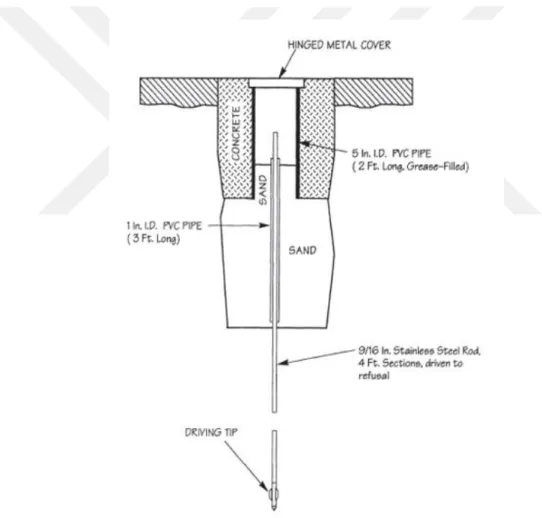
2.6.1. Three dimensional monuments

As the use of GNSS increased in 1993, the geodetic department began to set up new geodetic disks (Figure 2.1). Because of eventually the monument will be placed both ways, the disk has no reference as to its horizontal or vertical function. The position of the monument should not be an overhead obstacle or a surrounding obstacle that makes it difficult to set up or level with GNSS equipment (Anonymous5, 2007).

3. OVERVIEW OF GNSS

Global navigation satellite system (GNSS) is a system that utilizes satellites to give independent geospatial positioning. In other words, GNSS is a combined word of a navigation system which provides a user with a passive ranging three-dimensional positioning solution using radio signals broadcasted by orbiting satellites (Groves, 2008). There are some systems propose to cover worldwide. The most famous is the Navigation by Satellite Timing and Ranging (NAVSTAR) (GPS), the US government possesses and operates it (Groves, 2008). The European Galileo system and The Russian GLObal NAvigation Satellite System (GLONASS) systems are also operational (Teunissen and Montenbruck, 2017). The Indian Regional Navigation Satellite System (IRNSS) provides service to India and the neighboring area. Quasi-Zenith Satellite System (QZSS) is a local navigation satellite system that provides service to Japan and the Asia-Oceania region. The QZSS system is planned to be prepared in 2018. BeiDou (China) is the Chinese navigation satellite system. This system has 35 satellites. A local service was launched in December 2012. BeiDou is expanded to provide world-wide coverage by end of 2020 (Jeffrey, 2015).

3.1. Global Positioning System (GPS) 3.1.1. GPS history

GPS is the oldest and most widely used GNSS system (Awange, 2012; Ghilani and Wolf, 2015). The U.S. Department of Defense designed and built, operates and maintains the GPS (Xu, 2007). After World War II, the Pentagon made it clear that it needed to find solutions to exact and absolute positioning problems. Transit, Timation, Loran, Decca and many other projects and experiments have been conducted over the last 25 years. All the projects were able to determine the location was limited in terms of its accuracy or functionality (Anonymous6, 1999). The development of GPS system began in 1973, with the first satellite launch in 1978 and full world-wide operational ability attained in 1993 (Madry, 2015). Jeffrey (2015) stated that, in the beginning, before GPS was expanded to civilian use until 1983 GPS was accessible only for military use.

3.1.2. GPS segments

The space segment, control segment, and user segment are three segments of the GPS. There are 27 satellites in the space segment, on six orbital planes surrounding the

equator. Extra four additional satellites are kept in reserve (Jeffrey, 2015; Teunissen and Montenbruck, 2017). The orbital planes are tilted at 55° from the equator (see Figure 3.1a & 3.1b). According to Ghilani and Wolf (2015), this configuration provides 24-hour satellite coverage from latitude 80 ° N to 80 ° S. The average altitude of the satellite is 20,200 km above the Earth that travel in near-circular orbits and an orbital period of 12 sidereal hours.

(a) (b)

Figure 3.1. (a) The GPS Constellation and (b) a GPS Satellite (Ghilani and Wolf, 2015)

On the two carrier frequencies, each of the GPS satellites continuously transmits a single signal. The signals of the carrier frequency, which are broadcasted in the L band of microwave radio frequencies, are known as the L1 and L2 signals with frequencies of 1575.42 MHz and 1227.60 MHz, respectively. From a fundamental frequency, these

frequencies are derived, 𝑓₀ of the atomic clocks, which is 10.23 MHz. The L1 and L2

bands have frequency of 154𝑓0 and 120𝑓0, respectively. On these carrier waves, various

kinds of information (messages) are modulated using a phase modulation technique. According to Sickle (2015), in the broadcast message containing the ionospheric correction coefficients, almanac, satellite clock correction coefficients, broadcast ephemeris, and satellite health included. To independently determine the station’s position, the receiver occupies in real time, it was crucial to improve a system for accurately measuring the signal propagation time from a satellite to the receiver. In GPS, this has been achieved by modulating the carriers with pseudorandom noise (PRN) codes.

The PRN code consists of a unique sequence of randomly visible binary values (0 and 1) but actually generated with respect a special mathematical algorithm using devices known as tapped feedback shift registers. There are different PRN codes are transmitted by satellites. The L1 frequency is modulated with the precise code, or P code, and with the course/acquisition code, or C/A code. This C/A code allows receivers to allow the satellites and determine their approximate positions. Until recently, the L2 frequency was only modulated with the P code. The C/A and P codes are old technology. Modernized satellites will be equipped with new codes. The modernized satellites contain a second civil code for the L2 signal called L2C (Ghilani and Wolf, 2015; Jeffrey, 2015; Sickle, 2015; Teunissen and Montenbruck, 2017)

According to Jeffrey (2015), the L2C signal is expected to be available in 2018 from 24 satellites. This code has a civilian moderate (CM) and civilian long (CL) version. In addition, P-code is replaced by two new military code known as M code. In 1999, a third civilian signal (L5) was added by the Interagency GPS Executive Board (IGEB) to ensure security of life applications to GPS. L5 is broadcasted at a frequency of 1176.45 MHz. The L5 signal will carry both civilian codes along with a codeless component (Figure. 3.2). This feature will greatly increase the strength of the signal due to different processing techniques (Ghilani and Wolf, 2015; Sickle, 2015; Teunissen and Montenbruck, 2017). The last civil GPS signal L1C is designed for the next production GPS satellites (Jeffrey, 2015).

Control segments consist of a master control station (and a backup master control station), monitor stations, ground antennas and remote tracking stations, as shown in Figure 3.3. Teunissen and Montenbruck (2017) stated that, there are 16 worldwide monitoring stations; ten of the National Agency for Geospatial Intelligence (NGA) and six of the US Air Force. The monitor station monitors satellites through broadcast signals, including satellite ephemeris data, almanac data, clock data and ranging signals. The master control station takes the signal after sending from monitor station to recalculate the ephemeris. Through data up-loading stations the results are resent to the satellites (Jeffrey, 2015; Teunissen and Montenbruck, 2017).

Figure. 3.3. GPS control segment (Teunissen and Montenbruck, 2017)

The User Segment includes everyone using a GPS receiver to take the signal of the GPS and find their location and/ or time. Common applications in the user segment includes surveying, land navigation for hikers, aerial navigation, vehicle location, marine navigation, machine control etc (Anonymous6, 1999).

3.2. GLObal NAvigation Satellite System (GLONASS)

Initially, GLONASS was accessible only for military use, which is developed by the Union of Soviet Socialist Republics (USSR), then used in civil positioning survey like GPS. The first satellite was launched in 1982. GLONASS development was continued by Russia, after the dissolution of the Soviet Union in 1995 full satellite constellation completed. In 2001, due to a relatively the satellites short lifetime and the financial

problems, the constellation was then permitted to decay, reaching a nadir of seven satellites. The GLONASS has 24 satellites in orbits with 3 active spares, It is uniformly arranged on three orbital planes with a nominal inclination angle of 64.8° with the equatorial plane of the earth (Groves, 2008; Jeffrey, 2015). The altitude of the satellite's orbit is 19,100 km and have a period of approximately 11.25 hr. Or according to Teunissen and Montenbruck (2017) equal to 11h15 min 44s ± 5s. At least five satellites are always visible to users (Ghilani and Wolf, 2015).

To know the GLONASS services, some details about the signal here are important. Hofmann-Wellenhof et al. (2008) point out that all GLONASS satellites continuously provide navigation signals: the standard- accuracy signal, i.e. the C/A-code (also denoted as S-code), and the high accuracy signal, i.e., the P-code, in two sub bands of the L-band, denoted as G1 and G2. Note that this denotation allows a very difference between the GPS carriers L1 and L2 and GLONASS bands. Nevertheless, as literature, L1 (1598.0625-1609.3125 MHz) and L2 (1242.9375-1251.6875 MHz) are sometimes employed in GLONASS. G1 is modulated by the C/A-code, while G1 and G2 are modulated by P-code. GLONASS's upgrading process has been added a standard accuracy signal to the G2 of the GLONASS-M satellite. The wavelength of C/A-code of GLONASS is about 600m and the wavelength of P-code approximately 60m (Hofmann-Wellenhof et al., 2008).

The GLONASS control segment consists of the system control center and a network of command tracking stations across Russia. The GLONASS control segment, like GPS, controls the health of the satellites, the ephemeris corrections determination, like the satellite clock offsets respecting GLONASS time and Coordinated Universal Time (UTC). Corrections are sent to the satellites by the control center two times a day (Jeffrey, 2015).

3.3. Reference Coordinate Systems

According to Ghilani and Wolf (2015), three various reference coordinate systems are significant when the point’s position on Earth is determined from satellite observations. First, the satellite position now observed is indicated in the space satellite reference coordinate system. This 3D rectangular coordinate system is represented by the satellite's orbit. After that, it is transformed into a 3D rectangular geocentric coordinate system, which is correlated to the physical shape of the Earth, because of the locations of

new points are determined on the surface of the Earth. In the end, the geocentric coordinates are converted into the most often used and locally geodetic coordinate system (Ghilani and Wolf, 2015).

Uren and Price (2010) stated that, the datum used for GNSS positioning is called World Geodetic System 1984 (WGS84). The WGS84 ellipsoid is the foundation of the coordinate system. By the U.S. Military since January 21, 1987, this datum has been used. However, there have been six incarnations of WGS84 since then. The particular version of the datum has changed. WGS84 (G1762) is the latest version of WGS84 at the time of this writing. Where G is the GNSS's week number when that the coordinates first were used in the National Geospatial-Intelligence Agency (NGA) precise ephemeris estimations. So today, GNSS receivers determine coordinates according to the sixth and latest update to the WGS84 that is G1762.

According to Sickle (2015), from more than 1900 Doppler stations observations were made to produce the first WGS84. It was reviewed to become WGS84 (G730) to integrate GPS observations. On 29/6/1994, the GPS operational control segment (OCS) has applied this realization. More GPS-based realizations of WGS84 followed, on 29/1/1997 WGS84 (G873), on 20/1/2002 WGS84 (G1150), and on 8/2/2012 WGS84 (G1674) were implemented. Today’s epoch of WGS84 is (G1762).

3.4. GNSS Positioning

Fixing the position in three dimensions may involve measuring range (or distance) from three or more satellites whose X, Y, and Z positions are known to determine the user’s X, Y, and Z positions. In its easiest method, the range R between satellite and receiver is computed based on the differences between satellites and receivers in time,

departure time (𝑡𝐷) is the time that the satellites broadcast signals, arrival time (𝑡𝐴) is the

time that the receivers take the signals. Then the time to receive the signal from the

satellite to the receiver is (𝑡𝐴 − 𝑡𝐷) = ∆t, which is called the delay time. The range R

between satellite and receiver is computed from

R = (𝑡_𝐴 − 𝑡_𝐷)c = ∆t c (3.1)

Where c = the velocity of light, that is equal to 3 × 108 _{𝑚 𝑠⁄}

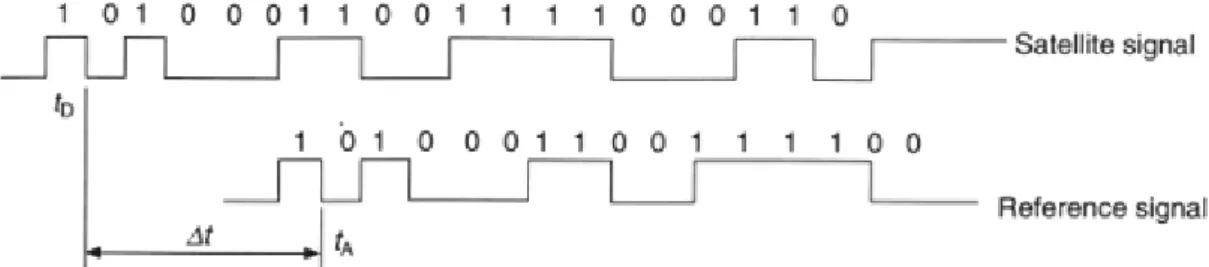
Acoording to Schofield and Breach (2007), while the above defines the basic principle of range measurement, to attain it one would require the receiver should be perfectly synchronized with the same clock as the satellite. This uses a pseudorandom

binary code (P or C/A), usually a correlation procedure using 'C / A', because it makes the receiver very expensive. The signal of the satellite reaches the receiver and the receiver begins to generating its own same C/A code. The receiver-generated code is cross-correlated with the satellite code (Figure 3.4). The receiver can create the same received satellite code; therefore, it can calculate the time delay (Δt). Nevertheless, inexpensive receiver clocks are not necessary, but it does not remove the exact synchronization problem of the two clocks. Therefore, the difference between the two

clocks in time is called clock bias, due to a wrong estimate of ∆t.

The calculated ranges are called ‘pseudo-ranges’. The effects of clock bias can be removed by using four satellites. By the difference in coordinates X, Y and Z system, the range is defined as: -

𝑅 = (∆𝑋2 _{+ ∆𝑌}2_{+ ∆𝑍}2₎1_{2 (3.2)} If the error in R, due to clock bias, is 𝛿𝑅 and is constant throughout, then:

𝑅1+ 𝛿𝑅 = [(𝑋1− 𝑋𝑃)2+ (𝑌1− 𝑌𝑃)2+ (𝑍1− 𝑍𝑃)2] 1 2 𝑅₂+ 𝛿𝑅 = [(𝑋₂− 𝑋_𝑃)2_{+ (𝑌} 2− 𝑌𝑃)2+ (𝑍2− 𝑍𝑃)2] 1 2 _(3.3) 𝑅₃+ 𝛿𝑅 = [(𝑋₃− 𝑋_𝑃)2_{+ (𝑌} 3− 𝑌𝑃)2+ (𝑍3− 𝑍𝑃)2] 1 2 𝑅4+ 𝛿𝑅 = [(𝑋1− 𝑋𝑃)2+ (𝑌1− 𝑌𝑃)2+ (𝑍1− 𝑍𝑃)2] 1 2

Where 𝑋𝑛, 𝑌𝑛, 𝑍𝑛 = the coordinates of satellites 1, 2, 3 and 4 (n = 1 to 4) 𝑋𝑝, 𝑌𝑝, 𝑍𝑝 = the coordinates required for point P

Rn = the measured ranges to the satellites

Solving the four equations for the four unknowns 𝑋𝑝, 𝑌𝑝, 𝑍𝑝 and 𝛿𝑅 also solves for the error due to clock bias (Schofield and Breach, 2007):

Observing the phase shift of the satellite signal makes it possible to improve the accuracy of the measurement range from the satellite to the receiver. In this approach, the phase-shift in the signal that happens, from the second it is broadcasted the signal by the satellite until the receiver received the signal. However, it does not take into account the complete wavelength or number of cycles that occur as the signal travels between the satellite and the receiver. Schofield and Breach (2007) stated that, this number is known as the integer ambiguity. Because satellites use one-way communication, the ambiguity cannot be determined by transmitting additional frequencies because the satellites are moving and their range is constantly changing. To determine the ambiguity, several methods are used; all these methods require extra observations. The mathematical model for carrier phase-shift, corrected for clock biases, is

𝛷_𝑖𝑗(𝑡) =1_𝜆𝜌_𝑖𝑗(𝑡) + 𝑁_𝑖𝑗 + 𝑓𝑗_[𝛿𝑗_{(𝑡) − 𝛿}

𝑖(𝑡)] (3.4)

where for any particular epoch in time, t, 𝛷_𝑖𝑗(𝑡) is the carrier phase-shift

measurement between satellite j and receiver 𝑖, 𝑓𝑗 _{is the frequency of the broadcast signal}

generated by satellite j, 𝛿𝑗_{(𝑡). The clock bias for satellite j, 𝜆 is the wavelength of the}

signal, 𝜌_𝑖𝑗(𝑡) is the geometric range between receiver 𝑖 and satellite j, 𝑁_𝑖𝑗 is the integer

ambiguity of the signal from satellite j to receiver 𝑖, and 𝛿_𝑖(𝑡) is the receiver clock bias

(Ghilani and Wolf, 2015).

3.5. GNSS Error Sources

The position of a GNSS receiver is computed depend on received data from satellites. Nevertheless, various sources of error make the location computation wrong. Some of these errors, caused by the refraction of the satellite signal while passing through the ionosphere and the troposphere, or as the Government's Selective Availability (SA) methods are presented on purpose. The error’s kind and how it is moderated is significant to compute the precise location, since the level of precision is only useful to the extent that the measurement can be trusted (Jeffrey, 2015).

3.5.1. Satellite clocks

According to Jeffrey (2015), atomic clocks in GNSS satellites are so precise, but float a small amount. Unfortunately, small errors in the satellite clock make amount errors in the location calculated by the GNSS receiver. Like a clock error of 10 nanoseconds results in a position error of 3 meters. The GNSS ground control station monitors the satellite clock and compares with a more precise clock worked in it. The estimated clock shift is provided by the satellite in the download data normally, the estimated value has a precision of approximately ± 2 meters, and precision may differ by various GNSS systems. In order to achieve a higher precise location, the GNSS receiver should compensate the clock error. By downloading precise satellite clock information from the Space-Based Enhancement System (SBAS) or Precise Positioning (PPP) service provider, the clock errors are compensated. Accurate satellite clock information includes clock error correction calculated by SBAS or PPP system. using a differential GNSS or real time kinematic (RTK) configuration is another way to compensate for clock errors (Jeffrey, 2015).

3.5.2. Orbit errors

GNSS satellites move on its own very precise orbits. However, such as the satellite clock, the orbits do vary a small amount. In addition, like satellite clocks, small changes in orbits cause large errors in the computed locations. Jeffrey (2015) stated that, the satellite orbit is continuously monitored by the GNSS ground control system and sends a correction to the satellites, if the satellite orbit shifts, and the satellite ephemeris is corrected. Despite sending corrections from GNSS ground control system, there are still minor errors in the orbit, which can cause position errors of up to ± 2.5 meters. By downloading precise ephemeris information from an SBAS system or PPP service provider satellite orbit errors are compensated or by using Differential GNSS or RTK receiver configuration (Jeffrey, 2015).

3.5.3. Ionosphere and tropospheric error

One of the layers of the atmosphere is the ionosphere that is between 80 km and 600 km above the earth. Ions are electrically charged particles in the ionosphere layer. These ions delay the signals of the satellite. Another layer of the atmosphere is the troposphere. This layer is the closest layer to the Earth’s surface. Due to changing

humidity, temperature and atmospheric pressure in the troposphere, the tropospheric delay occurs (Jeffrey, 2015). The errors worsen for instance signals passage from directly overhead to down near the horizon. According to Kavanagh and Mastin (2014), by planning night time observations, using short baseline lengths (1–5 km) and by gathering adequate redundant data or by collecting data on both frequencies over long distances (20 km or more) these errors can be reduced. Most surveying agencies do not store observations from satellites below the cutoff angle of (10–15°).

3.5.4. Multipath error

The main error source for GNSS surveying is multipath. The multipath error happens while the signal of the satellites reaches the antenna of the receiver in various ways (Figure 3.5). These ways may be reflected signals the direct line of sight signal from objects around the antenna of the receiver (El-Rabbany, 2002).

According to Jeffrey (2015), the easiest way to decrease multipath errors is to set up the antenna of the GNSS receiver apart from the reflective surface. While this is not feasible, the antenna of the GNSS receiver should handle the multipath signals. Due to the new technology needed to process multipath signals, it is better for high-end GNSS receivers and antennas to refuse multipath errors.

3.5.5. Other error sources

Some other minor error sources contributing to the receiver's location error. These include (1) satellite ephemeris errors; the future satellites locations can be forecasted by the broadcast ephemeris. Nevertheless, due to changes in gravity, solar radiation pressure, and other exceptions, these expected orbital positions are always containing error. In the code-matching method, these satellite-positioning errors are immediately converted into the calculated locations of receivers. By using updated ephemeris this problem can be reduced, depend on the exact locations of the satellites are determined by monitoring stations (Ghilani and Wolf, 2015). A disadvantage of that is the updated data is getting late. After survey, three updated ephemerides are available: first, ultra-rapid ephemeris that is available twice a day, second, the rapid ephemeris is available within two days when the survey is finished, and the last, the precise ephemeris is the most precise is available two weeks after completed the survey. The ultra-rapid or rapid

ephemerides are adequate for most surveying projects (Ghilani and Wolf, 2015). (2) Receiver noise; Receiver noise is the error of position made by the GNSS

receiver's hardware and software. High-end GNSS receivers have less receiver noise than lower cost GNSS receivers. (3) Another error source in GNSS surveying is to observe the antenna height above the occupied point. The observations are made to the datum point of the ground station. In the case of the inclined height, it must be observed in several places around the ground surface, and if the observations are not accepted, the level of the instrument must be checked. The software in the system changes the slanted height to the vertical distance of the antenna above the station (Ghilani and Wolf, 2015).

3.6. Satellite Geometry and Dilution of Precision in GNSS

Another error source in GNSS surveying is the geometry of the visible satellites at the time of survey. Like the situation in traditional surveys, the accuracies of computed positions are affected by the geometry of the network of observed ground stations. Figure 3.6 shows the angles between satellites at the time of observation. As shown in Figure 3.6(a), the meaning of weak geometry is the small angle between satellite signals at the time of observations and usually at calculated locations that contain larger errors. Conversely, strong geometry, see Figure 3.6(b), an improved solution is achieved when the angles between incoming satellite signals are not small. By performing least-squares

adjustment the expected accuracy due to satellite geometry is determined (Ghilani and Wolf, 2015).

El-Rabbany (2002) stated that, the dilution of precision (DOP) is a single dimensionless number that can measure the effect the satellite geometry. There are a number of types of DOP measurements: horizontal (HDOP), vertical (VDOP), time (TDOP), relative (RDOP), and the two most commonly used in surveying geometric (GDOP) and position (PDOP) (Seeber, 2003).

GDOP =√(PDOP)2_{+ (TDOP)}2 _(3.5) The worse the geometry of the satellites, the higher the DOP value will be, providing a lower certainty of the solution. For PDOP, usually a value of six or less is wanted when obtaining a position. Nowadays, due to large number of available satellites, the PDOP will usually be around two in open area (Figure 3.6a & 3.6b). If obstacles block a part of the sky where there are enough satellites for a solution, they are all within a range of the sky, which is a very weak solution and a high DOP (Kavanagh and Mastin, 2014).

Figure 3.6a. Poor GDOP Figure 3.6b. Good GDOP

3.7. GNSS Positioning Modes

Positioning by GNSS can be done in two techniques: point positioning or relative positioning. According to El-Rabbany (2002), GNSS point positioning includes just a GNSS receiver simultaneously tracks at least four satellites to find its own positions with respect to the Earth’s center. To determine the receiver’s position, GNSS receiver

measures the code pseudo ranges (El-Rabbany, 2002). when a relatively low accuracy is required such in navigation, an accuracy of better than 20 m (Schofield and Breach, 2007).

However, GNSS relative positioning operates two GNSS receivers that track the same satellite at the same time. If two receivers track four or more identical satellites can be obtained, a positioning accuracy level of a sub centimeter to a few meters. According to the desired accuracy, carrier-phase or/and pseudo range measurements can be used in GNSS relative positioning. The highest achievable accuracy is achieved in this method. GNSS relative positioning can be done in post-processing or real time modes. This method is applied for high precision applications such as mapping, surveying, precise navigation, and GIS (El-Rabbany, 2002).

3.8. Field Procedures in GNSS Surveys

Depending on the type of survey and the abilities of the receiver field procedures are performed. Currently, a number of methods in the field procedures being used in surveying that is kinematic, pseudo kinematic, rapid static and static methods. All are depending on carrier phase-shift measurements and use relative positioning techniques; that is, at least two receivers, setting up on various stations and observing at the same time to the same satellites. The distance (range) between receivers known as a baseline,

and from the observations its 𝑑𝑋, 𝑑𝑌, and 𝑑𝑍 coordinate differences are calculated

(Ghilani and Wolf, 2015).

3.8.1. Static method

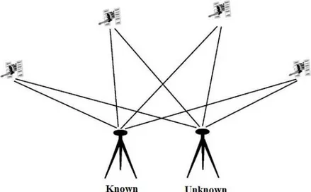
Static GNSS surveying method is a relative positioning method that based on the carrier-phase measurements (El-Rabbany, 2002). In order to obtain high accuracy over long distance like in geodetic control surveys this method is used (Schofield and Breach, 2007). In this method two or more occupied receivers at the same time tracking the same satellites (Figure 3.6). The base receiver is occupied to a station with accurately known values. Another receiver is occupied to a point whose values are unknown. Any number of receivers can be supported by the base receiver (El-Rabbany, 2002).

Figure 3.6. Static GNSS surveying (El-Rabbany, 2002)

In principle, static GNSS surveying depends on receiving data from satellite signals at both the base and other receivers simultaneously for a specific time, after post-processing the collected data the values of the unknown point are computed (El-Rabbany, 2002). According to the baseline length, the satellites number, the GDOP and the type of equipment the occupation time is planned. Occupation time should be long adequately to certainly fix the integer ambiguity in the baseline solution; therefore; the more satellites over the project area the more reliable and faster the integer can be fixed (Manual, 2003). Station occupation time is different for example, according to the Hofmann-Wellenhof et al. (2008) and Ghilani and Wolf (2015), using dual ferequency equal to (20 min + 2 min/km) and El-Rabbany (2002) says 20 minutes to a few hours, and according to Schofield and Breach (2007), observation times can change from 45 min to some hours. A good rule of thumb is 5 minutes per kilometer of baseline length with a minimum of 15 minutes. The epoch sampling rate in a static method should be the same for all receivers at the time of the survey. Normally, epoch rate is 15 secs to reduce the number of data, and so the memory card are required (Ghilani and Wolf, 2015).

Relative accuracies with static method are about ±(3 to 5 mm +1 ppm) (Ghilani and Wolf, 2015). Or 5 mm + 0.5 ppm of the baseline length and 10 mm + 0.5 ppm vertically. The ppm or parts per million components (equivalent to 1mm per km) (Uren and Price, 2010). Manual (2003) stated that, if the length of baselines between 1 to 100 km, the accuracy is 10 mm + 2 ppm or better.

3.9. Mission Planning

Sickle (2015) points out that, an important consideration in planning a GNSS survey is the satellites location above an observer’s horizon. Therefore, most software provides different ways of showing the satellite geometry for a specific site over a specified period. For instance, the geometry of the satellites over a time span of the observation is significant; as the DOP alterations, satellites move. The DOP may be already worked. DOP can be expected. It depends on the angle between GNSS satellites to the receivers, and they can also afford the associated DOP factors because of most GNSS software let calculation of the satellite geometry from any given location and time (Sickle, 2015).

Another significant action in scheduling surveys is choosing suitable observation windows, that is consists of determining the number of satellites, which will be visible from a project area during a planned observation time. Within the planned schema, using almanac data azimuth and elevation angles to each visible satellites approximately are determined. Furthermore, to observing date and time, the necessary computer input, include the estimated geodetic coordinate of the station, and approximately existing satellite almanac (Ghilani and Wolf, 2015).

3.10. Observation Scheme and Redundancy

For control surveying projects, after existing nearby control points are located and the new control points established, and the measurements are executed comprise what is termed a network. According to the type, and scope of the surveying project, the network may differ from a very big and complex configuration to only a few stations.

Ghilani & Wolf (2015) stated that, after establishing the stations, an observation scheme is designed to carry out the work. This scheme consists of a series of scheduled observation sessions to achieve the objectives of the survey most efficiently. At least, all stations on the network must be connected to at least one other station with a non-trivial baseline as described later. However, for checking and improving the reliability, and precision of the network, the schema also needs to include several redundant baseline observations (i.e., repeat observations of certain baselines, multiple occupations of stations, and baseline observations between existing control stations) to be used. The main factor for determining the amount and method of redundant measurements is the required precision. The necessity of the number and types of redundant observations to achieve

AA, A, B and C accuracy orders caused that the Federal Geodetic Control Subcommittee (FGCS) has published some of criteria and specifications for GNSS relative positioning. For high-precision projects, typically larger, these criteria and specifications or other like criteria manage the performance of surveys and should be followed precisely (Ghilani and Wolf, 2015).

In GNSS relative positioning, the number of nontrivial (independent) baselines for one session is equal to the number of receivers which used in the session minus one, or

b = r-1 (3.6) Where b is the number of independent baselines and r is the used receivers in the session. If in a session only two receivers are used, the observed baseline is nontrivial. If more than two receivers are used, trivial and nontrivial (mathematically dependent) baselines are result. Using four receivers in one session results in six baselines: three nontrivial and three trivial. It is important to distinguish between baselines because nontrivial baselines can only be considered. The network should not contain trivial vectors of multiple GNSS receiver sessions. However, when the decision is made, as a baseline, only three are included in the network (Ghilani and Wolf, 2015; Sickle, 2015). Trivial baselines are supposed that the remaining baselines which are rejected. In practice, in a four-receiver session the three shortest baselines are always supposed the nontrivial baseline and the three longest baselines are removed as trivial baseline. The nontrivial baselines are not always the shortest baselines. Because of incomplete data, multipath, cycle slips, or some other weakness in the observations occasionally one of the shorter baselines is eliminated. After the data execution have been made, each session will require analysis before such decisions can be made (Sickle, 2015). The total number of trivial and nontrivial baselines:

𝑇 =𝑟(𝑟−1)₂ (3.7)

Where T is the total baselines (trivial and nontrivial) and r is the receiver’s number (Michael et al., 1995; Manual, 2003; Seeber, 2003; Ghilani and Wolf, 2015). The number of trivial baselines for any session is

𝑡 =(𝑟−1)(𝑟−2)₂ (3.8)

The goal of the survey, the desired accuracy, the number and performance of GNSS receivers available, and the logistic conditions are the main factors to select the measurement concept. Therefore a general classification is not easy and not possible.

If only two receivers were used there would be no trivial baselines and it might appear there would be no redundancy at all. However, to connect all stations with the nearest adjacent, receivers should be occupied any station more than once, and every time in a different session (Hull, 1989; Sickle, 2015). One possibility is to operate one receiver at a center of the stations, and the other receiver occupy the neighboring points in a star shape. The neighboring stations with central stations are connected through nontrivial baselines. Another possibility is to occupy adjacent stations and form triangles or squares. This method leads to a high relative accuracy (Seeber, 2003). Or in the hub shape (Anonymous1, 2014)

If three or more receivers were used the stations are connected through non-trivial baselines in the form of loop. For control network survey, for performing loop closure analysis the baselines should form as a closed geometric shape (Ghilani and Wolf, 2015). In the GNSS project, all measurements made at the same time during a given time period are called sessions. Any session should be linked to at least one other session of the network through one or more control points where measurements are performed in both sessions. For increasing the reliability, stability, and accuracy of the network, the number of identical stations should be increased. In a multi-session survey, while three or more receivers are used, designing a scheme observation becomes an optimization problem between reliability, precision, and economy. Some basic considerations are described here (Seeber, 2003). It is defined as,

r receivers number in a session, n stations number,

m number of repeat occupied stations in two various sessions, and s sessions number

𝑟 (𝑟 − 1)/2 total number of baselines in a session, and (𝑟 − 1) number of nontrivial baselines in a session.

The required number of sessions in a network is:

𝑠 = [𝑛−𝑚_𝑟−𝑚] (3.9)

s becomes the next largest integer. If each session has more than one occupied station, some baselines are determined twice. In the total network we have

𝑠 (𝑟 − 1) number of nontrivial baselines, and

(𝑠 − 1) (𝑚 − 1) number of nontrivial baselines which are double determined.

Having defined the number of sessions, the next problem in a network observation is to determine an optimized session schedule. A session schedule is defined as a series of successively observed sessions. If s represents the number of sessions for a given network, then possible session schedules will be given by the 𝑠!. For some networks, this will be a very large number given that projects typically deal with networks comprising of many points.

In four-point network all the possible baselines (sessions) that can be measured (six in total) without repeating any observations. For two receivers, that have been arbitrarily selected out of a possible 720 session schedules, the one particular schedule that will give the lowest cost from a specific cost matrix. The receiver movement costs between all the neighboring points in the network can be illustrated by a cost matrix, while each component in the matrix is a cost between two points. If the cost of moving between two points does not depend on the direction of movement. In practice, the non-symmetric cost matrix is realistic because the movement between points generally requires a combination of travel, walking and uphill travel compared to downhill travel. When an airplane is used to move between points, then the symmetric cost matrix may be more appropriate. Information gathering and research such as through reconnaissance or interpretation from satellite imagery can be used to collect data to enable costs between project points to be calculated (Ogaja, 2011).

GNSS control networks first, second, and third orders should be designed with adequate redundancy to identify and eliminate systematic errors and/or blunders. Redundancy of network design is attained by many way is different from one author to another; for example, related to Kuang (1996), the highest precision and reliability of a GNSS network are expected if all the possible combinations of baselines in the network would be measured. According to the Sickle (2008), to meet order AA geometric accuracy standards, the FGCC requires three or more occupations on 80% of the stations in a project. Three or more occupations are necessary on 40%, 20%, and 10% of the stations for A, B, and C standards, respectively. When the distance between a station and its azimuth mark is less than 2 km, both points must be occupied at least twice to meet any standard above second-order. Two or more occupations are required for all horizontal control stations in order AA the percentage requirements for repeat occupations on