ÇANKAYA UNIVERSITY
GRADUATE SCHOOL OF SOCIAL SCIENCES FINANCIAL ECONOMICS
MASTER THESIS
THE J-CURVE HYPOTHESIS: AN INVESTIGATION OF BILATERAL TRADE BETWEEN NIGERIA AND EUROPEAN UNION
ABUBAKAR KABIR BABA
Title of the Thesis: The J-curve Hypothesis: An Investigation of Bilateral Trade between Nigeria and European Union
Submitted by : Abubakar Kabir BABA
Approval of the Graduate School of Social Sciences, Çankaya University
Prof. Dr. Mehmet YAZICI
Director
I certify that this thesis satisfies all the requirements as a thesis for the degree of Master of Science.
Prof. Dr. Mehmet YAZICI
Head of Department
This is to certify that we have read this thesis and that in our opinion it is fully adequate, in scope and quality, as a thesis for the degree of Master Science.
Prof. Dr. Mehmet YAZICI
Supervisor
Examination Date: 13/01/2014 Examining Committee Members:
Prof. Dr. M. Qamarul ISLAM (Çankaya Univ.) --- Prof. Dr. Mehmet YAZICI (Çankaya Univ.) --- Prof. Dr. M. Mete DOĞANAY (Çankaya Univ.) ---
iii
STATEMENT OF NON PLAGIARISM
I hereby declare that all information in this document has been obtained and presented in accordance with academic rules and ethical conduct. I also declare that as required by thesis rules and conduct, I have fully cited and referenced all material and results that are not original to this work.
Name, Last Name: Abubakar Kabir BABA Signature:
iv
ABSTRACT
THE J-CURVE HYPOTHESIS: AN INVESTIGATION OF BILATERAL TRADE BETWEEN NIGERIA AND EUROPEAN UNION
BABA, Abubakar Kabir
M.Sc., Department of Economics Supervisor: Mehmet YAZICI, Ph.D.
January 2014, 122 pages
This thesis investigates the bilateral J-curve effects in the short-run and the Marshall–Lerner (ML) condition in the long-run between Nigeria and European Union in particular and between Nigeria and each of the countries that made up E.U.15. The study covers the period of fifty-six quarters (1999:Q1–2012:Q4) and employs Autoregressive Distributed Lag (ARDL - bounds-testing) approach to cointegration and error correction model to analyse the relationships. The study found no evidence of J-curve and also the Marshall–Lerner (ML) condition is not satisfied in the bilateral case between Nigeria and European Union, but found the evidence of J-curve in the bilateral cases between Nigeria and each of Austria, Denmark, Germany and Italy in the short-run, while in the long-run, the Marshall-Lerner (ML) condition exists only in the case of Luxemburg. The study concludes with strong support for the assertion that real exchange rate changes alone can only be used as a policy tool to design and control Nigeria’s trade balance if the naira is to be appreciated against the currencies of this group of countries. Keywords: J-curve, Marshall-Lerner (ML) condition , Trade balance, Exchange rate
v
ÖZET
J-EĞRİSİ HİPOTEZİ: NİJERYA VE AVRUPA BİRLİĞİ ARASINDAKİ İKİLİ TİCARET ÜZERİNE BİR İNCELEME
BABA, AbubakarKabir
Yüksek Lisans, İktisat Bölümü Tez Yöneticisi: Prof. Dr. Mehmet YAZICI
Ocak 2014, 122 sayfa
Bu tez, Nijerya ve AB ile Nijerya ve AB(15)’i oluşturan ülkelerin herbiri arasındaki ticarette, kısa vadede j-eğrisi etkisini ve uzun vadede Marshall-Lerner ( ML ) koşulunu incelemektedir. Çalışma ellialtı çeyreklik(1999:Q1 -2012:Q4 ) dönemi kapsamakta ve eşbütünleşme ve hata düzeltme modellemeye yönelik otoregresif dağıtılmış gecikme ( ARDL - sınır - testi) yaklaşımını kullanmaktadır. Çalışmada, Nijerya ve AB arasındaki ticarette j-eğrisi etkisine rastlanmamış ve Marshall - Lerner ( ML ) koşulunun da sağlanmadığı tespit edilmiştir. Nijerya ile AB(15)’i oluşturan ülkeler arasındaki ikili ticarete bakıldığında ise, j-eğrisi etkisine Nijerya’nın Avustırya, Danimarka, Almanya ve İtalya ile olan ikili ticaretinde rastlanmış ve Marsall-Lerner (ML) koşulu da sadece Nijerya’nın Luxemburg ile olan ticaretinde sağlanmıştır. Doviz kuru bu ülkelerle olan ticarette bir politika aracı olarak kullanılmak isteniyorsa, dış ticaret dengesini iyileştirmek için Naira bu ülkelerin paralarına karşı değer kazanmalıdır.
Anahtar Kelimeler: J-eğrisi, Marshall-Lerner (ML) koşulu, Dış ticaret dengesi, Döviz kuru
vi
AKNOWLEDGEMENTS
I would like to express my gratitude to my parents (Kabir Baba and Zainab Muhammad) for their love, guidance, and prayers throughout my life. I would also like to thanks my siblings for their constant supports and encouragements.
My deepest appreciation goes to my wife (Bilkisu) and my children (Muhammad Kabir and Fatima) for their love, caring, sacrifice, encouragements, patience and prayers throughout the programme period.
I am extremely grateful to my supervisor Prof. Dr. Mehmet Yazıcı for his guidance, advice, criticism, encouragements and insight throughout the research. I also want to appreciate the effort of Prof. Dr. M. Qamarul Islam who developed the algorithm I used in this study.
I would like to thank all my friends for their assistances, advices and encouragements.
I felt indebted to the Kano State Government which finance me to undergo this study with 100% scholarship, may Almighty Allah assist me to pay back the people of Kano more than what I receive from this Government.
vii
TABLE OF CONTENTS
STATEMENT OF NON PLAGIARISM ………... iii
ABSTRACT……… iv
ÖZET……… v
ACKNOWLEDGMENTS……….. vi
TABLE OF CONTENTS………... vii
LIST OF TABLES……….. ix
LIST OF FIGURES……… x
CHAPTERS: 1. INTRODUCTION……… 1
1.1. Background to the Study……… 1
1.2. The Nigerian Experience………. 5
1.3. Studies about Nigeria……….. 6
1.4. Objective of the Study………. 7
1.5. Justification for Data and Methodology Used in the Study.. 8
1.6. Significance of the Study……… 9
1.7. Organisation of the Study……….. 9
2. LITERATURE REVIEW………. 10
2.1. Introductıon………. 10
2.2. The Theoretical Frame Work on J-Curve Phenomenon…… 11
2.2.1. The J‐Curve Hypothesis………... 11
2.2.2. Aggregated Data Studies……….. 15
2.2.3. Disaggregated Data Studies……….. 16
2.2.4. Industry Level Data Studies... 17
2.2.5. Sectorial Data Studies……….. 19
2.2.6. Marshall-Lerner (ML) Condition………. 19
2.2.6.1. Mathematical Derivation of Marshall-Lerner (ML) Condition……….. 21
2.3. The Empirical Evidences on J-Curve Phenomenon………. 24
2.3.1. Empirical Studies Using Aggregated Data………... 24
2.3.2. Empirical Studies Using Disaggregated Data…….. 26
2.3.3. Empirical Studies Using Industry Level Data…….. 28
2.3.4. Empirical Studies Using Sectorial Data…………... 30
2.3.5. Relevant Empirical Studies to Nigeria……….. 31
2.3.6 Relevant Empirical Studies to European Union….. 34
2.4. Brief Discussion on the Literature Reviewed……….. 38
viii
3. MODEL AND DATA DESCRIPTION………. 40
3.1. Introductıon……….. 40
3.2. Trade Balance Model……… 48
3.3. Description and Sources of Data………. 53
3.3.1 Import, Export and Trade Volume Data………… 53
3.3.2 GDP Data……….. 58
3.3.3 CPI Data……… 60
3.3.4 Bilateral Nominal Exchange Rate Data (N.Ei)……. 64
3.3.5 Bilateral Real Exchange Rate (REXi)……… 65
3.3.6 Bilateral Real Effective Exchange Rate………. 65
4. THE EMPIRICAL ESTIMATION PROCEDURES, RESULTS ANALYSES AND INTERPRETATIONS……… 68
5. SUMMARY AND CONCLUSION……… 88
References………. 93
Appendices: A. Mathematical Derivation of Marshall-Lerner (ML) Condition……… 102
B. CUSUM and CUSUMSQ Diagrams……… 106
ix
LIST OF TABLES
Table 3.1. Nigeria’s Top Five Major Trading Partners
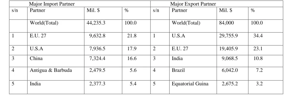
(values in mil. U.S.D) in Year 2010……… 41 Table 3.2. Nigeria’s Top Five Major Trading Partners
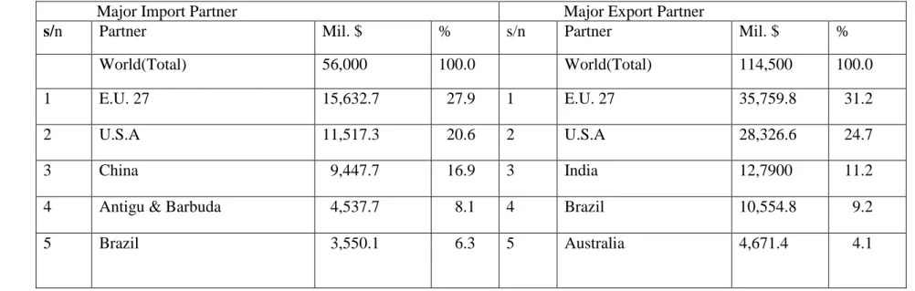
(values in mil. U.S.D) in Year 2011……… 42 Table 3.3. Nigeria’s Top Five Major Trading Partners
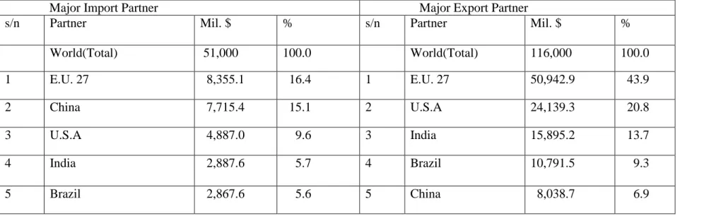
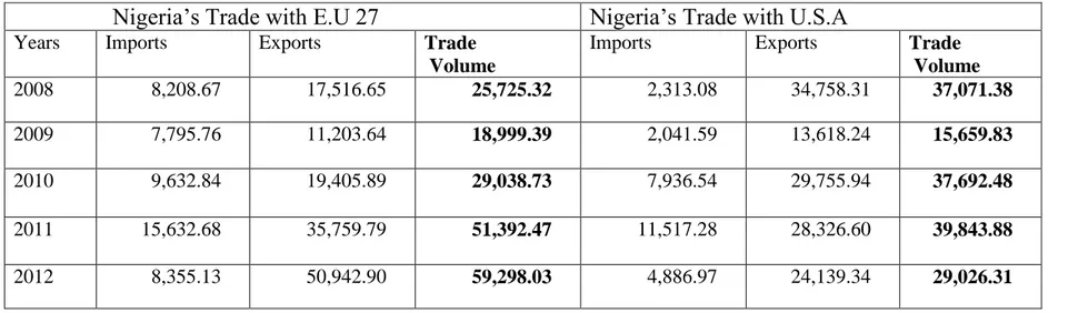
(values in mil. U.S.D) in Year 2012………. 43 Table 3.4. Nigeria’s Top Two Major Trading Partners
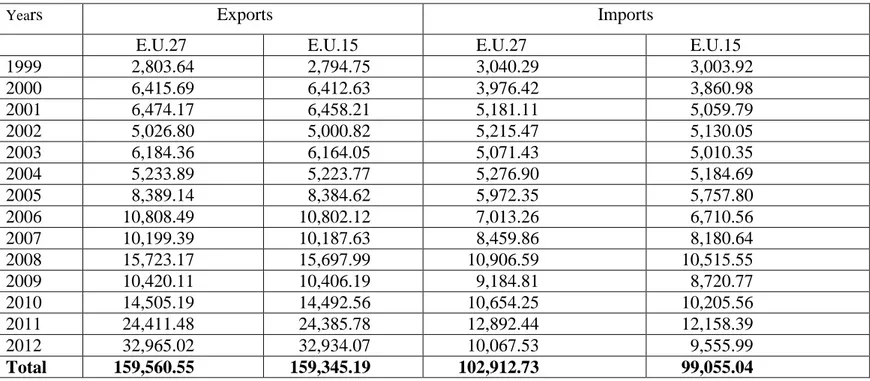
(values in mil. U.S.D) from Year 2008 – 2012…………... 44 Table 3.5. Nigeria’s Exports to and Imports from E.U.27 and
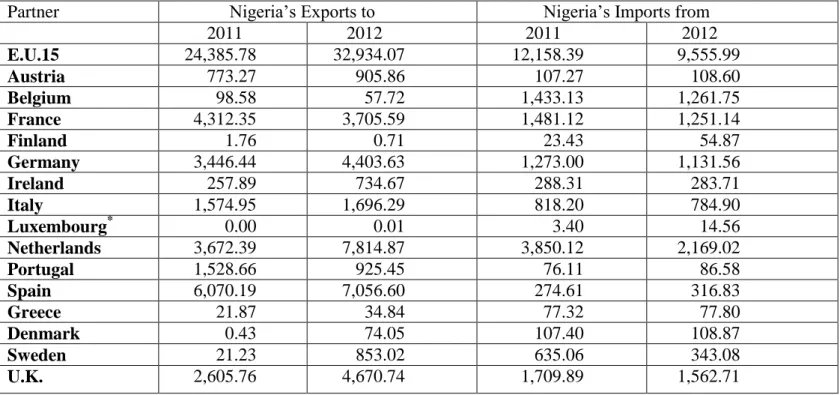
E.U.15 (values in mil. euro) from Year 1999 – 2012……. 45 Table 3.6. Nigeria’s Exports to and Imports from E.U.15 Members
(values in mil. euro) for Year 2011 and 2012……….. 47 Table 4.1. Calculated Diagnostic and Cointegration Tests Results
for Different Lag Length Imposed on the First-Differenced Variables……… 72 Table 4.2. Optimal Lag Orders Selection……….. 75 Table 4.3. Short-Run Coefficient Estimates of Exchange Rate
Variable………. 76 Table 4.4. Long-Run Coefficient Estimates……….. 81 Table 4.5. summary of cumulative sum and cumulative sum of the
x
LIST OF FIGURES
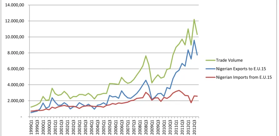
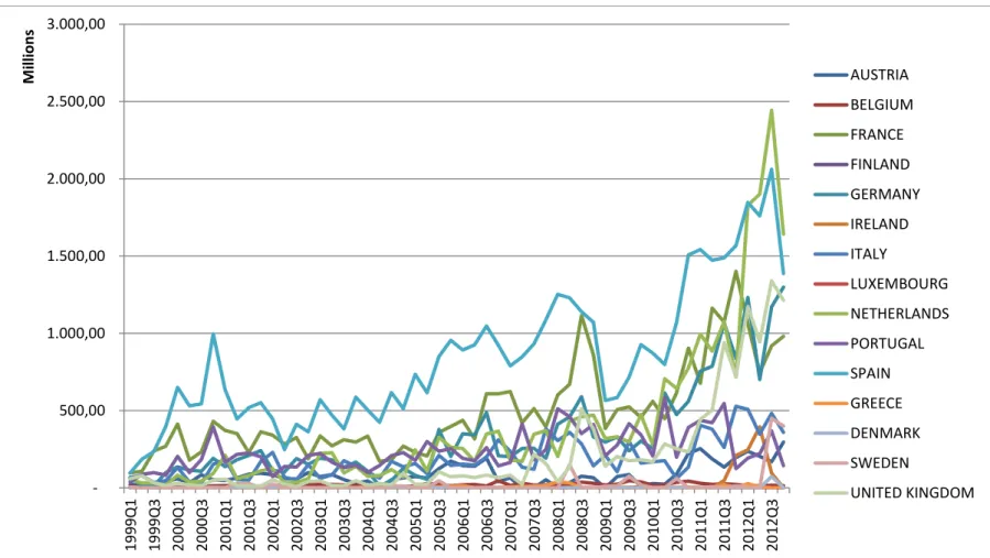
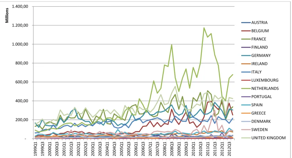
Figure 3.1. Nigeria’s Exports to and imports from E.U.15 and Their Trade Volume series (values in mil. euro)……54 Figure 3.2. Nigeria’s Bilateral Exports to countries under
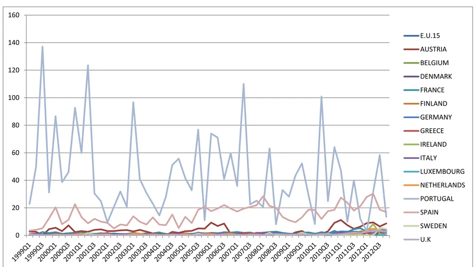
E.U.15 (values in mil. Euro)………. 56 Figure 3.3. Nigeria’s Bilateral Imports from countries under
E.U.15 (values in mil. Euro)………. 57 Figure 3.4. Bilateral Trade Balance between Nigeria and
countries Under E.U.15……… 59 Figure 3.5. Nigeria’s and E.U.15 Real Incomes’ series……… 61 Figure 3.6. Real Incomes’ series of countries under E.U.15
(values in mil. euro)……….. 62 Figure 3.7. Nigeria’s CPI and average E.U.15 CPI series….... 63
1
CHAPTER 1
INTRODUCTION
1.1 Background to the Study
A key relationship in international economics is that between trade balance and terms of trade. Understanding their dynamics is a major step toward creating an ideal trade policy. Whether depreciation actually helps improve trade deficits remain a key question that has drawn much scholarly attention. There exists a voluminous body of literature that has looked at the effect of currency depreciation on net exports of nations. Most of these centred on the concept of a ‘J-curve’ (Ghosh, 2012). “It is not clear if trade barriers and protectionism based on infant-industry arguments have achieved the desired changes in the trade balance. Much of the work centres on the twin concepts of the Marshall–Lerner (ML) condition and the J-curve phenomenon” (Bahmani-Oskooee and Ratha, 2004). For a country to improve its balance of trade, it needs to increase its competitiveness in international markets by devaluing its currency (if it uses fixed exchange rate system) or let its currency depreciate (if it uses flexible exchange rate system) against other currencies. But to benefit from currency depreciation/devaluation, a country needs to fulfil the Marshall– Lerner (ML) condition. The Marshall–Lerner (ML) condition - named after the two economists who discovered it independently, Alfred Marshall (1842-1924) and Abba Lerner (1903-1982), postulates that for a country to benefit from currency devaluation, the absolute sum of elasticities of demand for both import and export must be greater than unitary. The earlier literature developed on the relationship between currency devaluation and trade balance are on the agreement that this condition is necessary and sufficient for a successful
2
devaluation and are also interested in describing post-devaluation behaviour of a country’s trade balance in the long-run until the work of Maggi (1973) who first explained the short-run post-devaluation behaviour of the U.S. trade balance. He observed that the U.S. trade balance continued to deteriorate despite the authorities’ effort to control it through further devaluation in the short-run. He then explained the phenomenon and highlighted the implications of adjustment lags stemming from currency contracts, Pass-through, and quantity adjustments. He showed that these dynamics of the response of balance of trade to currency depreciation will trace out a j-shaped time path, which he eventually coined as ‘J-curve’. This is how the classical definition of the phenomenon is derived that the trade balance deteriorates and then improves following the real depreciation of currency in the short-run. Therefore, Bahmani-Oskooee and Bolhasani, (2008) asserts that “Thus, while earlier studies concentrated on testing the Marshall–Lerner condition, more recent studies have tried to distinguish the short-run effects of devaluation from its long-run effects and assess the validity of the J-Curve hypothesis”.
The text book definition of J-curve is now regarded as the classical definition of the phenomenon which expects the trade balance to deteriorate and then improve following the real depreciation of currency in the short-run. But Bahmani-Oskooee and Kovyryalova (2008) argue that
“This new definition of the J-Curve put forward by Rose and Yellen (1989) that the phenomenon can be defined to reflect short-run deterioration combine with the long-run improvement, seems to be closer to theory than the old one. Magee (1973) who originally introduced the concept conjectured that the trade balance can follow any pattern in the short run. Thus, short-run fluctuations in the trade balance combined with long-run improvements could constitute an even better definition of the J-Curve”.
Bahmani‐Oskooee is the earliest researcher that applies empirical methodology to investigate the phenomenon in the mid of 80s as argued by Bahmani-Oskooee and Ratha (2004) that
3
“Bahmani‐Oskooee is the first scholar to introduce the empirical methodology of testing the J‐Curve in 1985 when he applied the method on four countries, with different exchange rate regimes viz. Greece, India, Korea and Thailand. He defines the trade balance as the excess of exports over imports, imposes an Almon lag structure on the exchange rate variable, and adds world income, the level of domestic high powered money, and the level of the rest of the world high powered money to the multiplier-based analysis of the effects of exchange-rate change or devaluation provided by Kruger (1983), the methodology which he eventually corrects later in Bahmani-Oskooee (1989a) because of the inconsistency in the way the real exchange rate variable is defined above. Since P is the domestic price level, E should be defined as the number of units of domestic currency per unit of foreign currency rather than units of foreign currency per unit of domestic currency. Furthermore, he argues that any measure of real exchange rate must also include a measure of foreign price level. Thus defined, the exchange rate variable should have negative coefficients followed by positive ones to corroborate the J-curve phenomenon”.
The J-curve phenomenon has attracted the attentions of researchers from different parts of the world, considerably in the last four decades. Since the famous argument of Magee (1973) ‒ who theoretically claims that it is possible in the short-run trade balance to worsen and then improve following the real depreciation of currency in the short-run, various researchers developed interest and start investigating the phenomenon. The earlier group of empirical studies employed aggregate trade balance approach1, and they mostly used home country and rest of the world approach, thus suffer from aggregation bias as noted by Nazlioglu and Erdem (2011) that
“The problem associated with these studies is the employment of aggregate trade data, which potentially causes the so-called aggregation bias problem. The aggregation bias problem basically means that the significant effect of an explanatory variable on the dependent variable in some countries could be offset by the insignificant effect of the same variable in some other countries, thus (mis)leading to the conclusion that the variable in question would be insignificant in relation to the dependent variable”.
1
Magee (1973), Junz and Rhomberg (1973), Miles (1979), Kruger (1983), Himarios (1985), Bahmani-Oskooee (1985), Rosenweig and Koch (1988), Brissimis and Leventankis (1989), Bahmani-Oskooee (1989a).
4
To do away with this aggregation bias, researchers from the late 1980s shifted their attention to investigating disaggregated trade data2, as noted by Ardalani and Bahmani-Oskooee, (2007) that “because of the mixed conclusions, more recent studies have relied upon disaggregated data to test the phenomenon. Rose and Yellen (1989) was the first study to bring out the shortcomings associated with models using aggregate data and introduced a simple model that employed bilateral trade data between the United States and her six major trading partners”. To shed additional light on the short-run as well as the long-run relation between the exchange rate and the trade balance, Ardalani and Bahmani-Oskooee (2007) contemplated to employ a disaggregated trade data by using U.S monthly trade data of imports and exports at the commodity level of sixty-six industries for the period 1991- 2002.They investigate the short-run and the long-run effects of real depreciation of the dollar using error-correcting modelling technique. Though they were unable to find strong support for the J-Curve, their procedure has now become popular among researchers3, because of its power to deal with the so-called disaggregation bias as argued by Yazici and Islam (2011), that “the most recent trend now is to disaggregate the trade data further, with the aim of avoiding possible aggregation bias problem, by considering trade balance at commodity or industry level in bilateral trade with a trading partner”.
2
Rose and Yellen (1989), Wilson (2001), Baharumshah (2001), Bahmani-Oskooee and Kanitpong (2001), Hacker and Hatemi-J. (2003), Bahmani-Oskooee and Goswami (2003), Bahmani-Oskooee and Ratha (2004b), Halicioglu, (2007),
3
Bahmani-Oskooee and Kovyryalova (2008), Bahmani-Oskooee and Bolhasani (2008), Bahmani-Oskooee and Hegerty (2010), Yazici and Islam (2011), Soleymani and Saboori (2012), Verheyen (2012), and Bahmani–Oskooee and Hosny (2012) are some of the studies that followed their procedures.
5 1.2 The Nigerian Experience
Right from the independence, Nigeria had a persistent trade deficit, which turned to a surplus in 1966 with petroleum’s rapid growth as the major export commodity. In the late 1977 & 1978, demand for Nigeria’s crude oil decreased as oil became available from the U.S. and Mexico, and as global oil companies reacted to the less favourable participation terms offered by the Nigerian government. Since then the Nigeria’s trade balance improved up to early 1980s (1981-1983) when the trade deficit persisted. The trade balance continue to improve at a very volatile rate to date with the year 1998 only proved to be exception with deficit trade balance of ₦85,562m recorded4
. During this period Nigerian economy suffered quiet enough from the use of inappropriate exchange rate policies and exchange control regulations leading to an exchange rate transition due to structural changes in the economy, as explained by Sanusi (2004), that
“The fixed exchange rate regime induced an overvaluation of the naira and was supported by exchange control regulations that engendered significant distortions in the economy. That gave vent to massive importation of finished goods with the adverse consequences for domestic production, balance of payments position and the nation’s external reserves level. Moreover, the period was bedevilled by sharp practices perpetrated by dealers and end-users of foreign exchange. These and many other problems informed the adoption of a more flexible exchange rate regime in the context of the SAP, adopted in 1986”.
From 1986 to date Nigeria ditched the fixed exchange rate system and adopted floating exchange rate system with different exchange–rate arrangements in the quest of choosing the best policy that will improve its external sector. This is noted by Adeoye and Atanda (2012) when they explain that “The adoption of the International Monetary Fund (IMF) Structural Adjustment Programme (SAP) in 1986 resulted in the transition from fixed exchange rate regime to floating exchange rate regime in Nigeria”. Bala and
4
6 Asemota (2013), add that
“Nigeria has adopted different exchange–rate arrangements since its exit from fixed to flexible exchange–rate system. The frameworks employed in the FX market from 1986–2012 include: the dual exchange–rate system (1986–1987), the Dutch auction system (DAS) (1987), the unified exchange–rate system (1987–1992), and the fixed exchange–rate system (1992–1998). Others are the re– introduced DAS (1999–2002), the retail Dutch auction system (2002–2006), and the wholesale Dutch auction system (2006–to date)”.
Yet, devaluing naira is not just enough for the Nigeria’s external sector to improve. This is observed by Oladipupo and Onotaniyohuwo (2011), that “Exchange rate is a key determinant of the balance of payments
(BOP) position of any country. If it is judiciously utilized, it can serve as nominal anchor for price stability. Changes in exchange rate have direct effect on demand and supply of goods, investment, employment as well as distribution of income and wealth. When Nigeria started recording huge balance of payments deficits and very low level of foreign reserve in the 1980s, it was felt that a depreciation of the naira would relieve pressures on the balance of payments. Consequently, the naira was devalued. The irony of this policy instrument is that our foreign trade structure did not satisfy the condition for a successful balance of payment policy. The country’s foreign structure is characterized by export of crude petroleum and agricultural produce whose prices are predetermined in the world market and low import and export price elasticities of demand”.
1.3 Studies about Nigeria
In Nigeria, the literature on the relationship between exchange rate and trade balance have not receive much research attention, is rather scanty and ended with mixed conclusions, as highlighted by Godwin O. (2009), that “In Nigeria, previous studies carried out on the external sector
generally (e.g. Olisadebe, 1995; Egwaikhide, 1995; Egwaikhide, Chete and Falokun, 1994; Komolafe, 1996; Odusola and Akinlo, 1995; Orubu, 1988; Omotor and Jike, 2005; Omotor, 2008) and particularly on agricultural exports (e.g. Kwanashie, Ajilima and Garba, 1997; Omotor and Orubu, 2007) did neither address the theoretical issues nor the empirical evidence of the J-curve hypothesis”.
7
Some of the studies in Nigeria found the evidence of the classical J-curve5 and delayed J-Curve phenomenons6, some found no evidence at all7, while others found different shapes rather than the J-curve8. On the other hand, some studies couldn’t confirm the short-run relation evidence but rather the long-run relation9, while others claim that neither the short-run nor the long-run relation exist10.
It should be noted that all the studies above used aggregate data in their analysis. This reason has led us to argue that these inconclusive results could be due to aggregation. To the best of our knowledge no study in Nigeria has used disaggregated data to conduct bilateral study between Nigeria and its trading partner leaving the wide gap in Nigerian literature on the J-curve phenomenon.
1.4 Objective of the Study
At this juncture, this study will try to bridge the gap to investigate the existence of the bilateral J-curve by analysing both the short-run and the long-run impacts of exchange rate changes on bilateral trade between Nigeria and E.U and then disaggregating the study further by investigating the existence of the phenomenon between Nigeria and each of the countries that made up E.U.15 (Austria, Belgium, Denmark, Finland, France, Germany, Greece, Ireland, Italy, Luxembourg, Netherlands, Portugal, Spain, Sweden, U.K ). To accomplish this purpose, we estimate the trade balance model [The trade balance proposed by Rose and Yellen (1989), which models the real trade
5
Akonji et al (2013)
6
Kulkarni and Clarke (2009)
7
Umoru and Oseme (2013), Umoru and Eboreime (2013)
8
Godwin O. (2009), Joseph and Akhanolu (2011)
9
Oyinlola et al (2010), Bahmani-Oskooee and Gelan (2012)
10
8
balance to be a direct function of the real domestic income, real foreign income and real effective exchange rate, is closely followed in this study as it has become popular among researchers]11 on the total trade data between Nigeria and European Union (EU15) for the period of 1999:Q1–2012:Q4 by applying Autoregressive Distributed Lag (ARDL) approach to cointegration (i.e., the bounds testing cointegration approach) developed by Pesaran, Shin, and Smith (2001).
1.5 Justification for Data and Methodology Used in the Study
The study chooses the finite size of 15 trading partners in the European Union (E.U.15) and the period of fifty-six quarters (1999:Q1–2012:Q4). This is because E.U.27 (as a single economic union) has become the Nigeria’s major trading partner in recent years, and that this was the exact number of the union members as at 1st January, 1999 and the date also corresponds with Economic and Monetary Union (Euro-area) establishment date. Choosing E.U.15 as a proxy of E.U. is equally justified as they (E.U.15) cover a larger share of the Nigeria’s bilateral trade with E.U.27 with the total exports of Nigeria to E.U.15 reaches 99.87% of the total exports to E.U.27 from 1999-2012 while the total import from the same stands for 96.25% of the total imports from E.U.27 during the study period.
The Autoregressive Distributed Lag (ARDL) approach to cointegration and error correction model is used in this study because of the length and the nature of the data in question and also because of the objective to be achieved in the study. This approach (ARDL) has certain econometric advantages in
11
Example of these researchers include among others: Bahmani-Oskooee and Brooks (1999), Arora, et al (2003), Oskooee, and Goswami, (2003), Bahmani-Oskooee, and Ratha (2004b), Narayan (2004), Bahmani-Bahmani-Oskooee, et al (2006), Halicioglu, (2007), Ardalani and Bahmani-Oskooee (2007), Bahmani-Oskooee and Kovyryalova (2008), Bahmani-Oskooee and Bolhasani (2008), Baek et al (2009), Bahmani-Oskooee, and Kutan,(2009), Nazlioglu and Erdem (2011), Šimáková, J. (2012), Soleymani, and Saboori, (2012), and Umoru and Eboreime (2013).
9
comparison to other single cointegration procedures. Firstly, it avoids the endogeneity problems and inability to test hypotheses on the estimated coefficients in the long-run associated with the Engle-Granger (1987) method (Halicioglu, 2007). Secondly, the estimates from small sample sizes are super consistent (Narayan 2004). This approach also distinguishes the short-run effects from the long-run effects simultaneously (Bahmani-Oskooee, and Kovyryalova 2008), i.e captures both the short-run and the long-run effects of real depreciation on the trade balance. Lastly, it avoids need for unit root pre-testing for the classification of variables into I(1) or I(0), unlike standard cointegration tests (Bahmani-Oskooee and Brooks 1999).
1.6 Significance of the Study
The results of this study will have important policy implications. We hope this study improves our understanding of dynamic effects of exchange rate changes on Nigeria’s trade balance. It will also assist the policymakers to know that to what extent the real exchange rate changes shall be applied to design, control, forecast and manipulate trade flows in Nigeria and whether exchange rate can be a good indicator for monetary and exchange rate policies.
1.7 Organisation of the Study
This study is structured as follows. In the next chapter we review both theoretical and empirical literatures on the J-curve phenomenon. Following the literature study, the research methodology is identified for the research objective, trade balance model, data description and data sources are discussed in chapter three. The empirical estimation procedures and results are presented and discussed in chapter four, and finally, conclusions are drawn in the closing chapter.
10
CHAPTER 2
LITERATURE REVIEW
2.1 Introduction
The last four decades witness the era in which the literature on the J-curve phenomenon gathers momentum. The genesis of this phenomenon emanated when developed countries decided to allow demand and supply to determine the value of their currencies in the foreign exchange markets, such that the trade balance disturbances can be handled by the invisible hands. This is noted by Bahmani-Oskooee and Goswami (2003) that “In March 1973 when most industrial countries decided to float their currencies, it was believed that exchange rate flexibility would take care of trade deficits and isolate countries from disturbances originated abroad so that they could use fiscal and monetary policies to better manage their economies. The belief was mostly based on the fact that import and export demand elasticities are high enough to warrant improvement in the trade balance due to currency depreciation”. Magee (1973) is the first person to contemplate the phenomenon when he argued theoretically that it is possible in the short-run trade balance to worsen following the currency depreciation and eventually improve. He explains the phenomenon using three-stage lags: the currency-contract period, the pass through period, and the quantity adjustment period which he then coined as J-curve. From then on, researchers begin to investigate the short run as well as the long-run responses of trade balance to currency depreciation. This is stress by Bahmani-Oskooee and Goswami (2003) that
“Since such a short-run pattern resembles the letter J, it is known as the J-curve phenomenon in the literature. Owing to this concept, most studies in the 1980s and 1990s concentrated on establishing a direct link between the trade balance and the exchange rate. Such practice was considered to be relatively more attractive due to the fact that it
11
allowed the researchers to investigate the short-run response of the trade balance to exchange rate changes in addition to its long-run response. Bahmani-Oskooee (1985), Rosensweig and Koch (1988), Himarios (1989), and Bahmani-Oskooee and Malixi (1992) are some examples in this group with mixed conclusions”.
This section will review both the theoretical and empirical literatures in the development of J-curve phenomenon and then review relevant empirical studies to Nigeria and European Union countries.
2.2 The Theoretical Frame Work on J-Curve Phenomenon
2.2.1 The J‐Curve Hypothesis
The J-curve is a concept that explains the post-devaluation behaviour of a country’s trade balance in the short run. Due to adjustment lags, after devaluation or depreciation a country’s trade balance keeps deteriorating and then begins to improve, but only after a while. How long it takes for the trade balance to deteriorate, is an empirical question (Bahmani-Oskooee and Gelan, 2012). Magee (1973) was the first person to describe the phenomenon when he analysed the US monthly trade data from 1969 to1973. He explains the phenomenon using three-stage lags: currency contracts, pass-through, and quantity adjustments. Bahmani-Oskooee and Ratha (2004) noted that
“US trade balance deteriorated from a surplus of $2.2 billion in 1970 to a deficit of $2.7 billion in 1971. The authorities sought to correct this by devaluing the dollar in 1971. This, however, did not help, as the trade balance deteriorated even further (to a deficit of $6.8 billion) in 1972. Magee (1973) explains this pattern in terms of adjustment lags. He analyses the implications of (a) currency-contracts signed prior to devaluation, (b) newer currency-contracts signed after devaluation, namely, the periods of pass-through, and finally, and (c) the sluggish quantity adjustments”.
Godwin O. (2009) explains that the currency-contract period is the short period of time which follows ostensibly after the devaluation exercise. This short period is the immediate era that characterizes the exchange-rate variation
12
associated with the devaluation given that there are previously made contracts before the variation occurs. The “perverse valuation” worsens the initial trade balance as domestic currency prices of imports rise. The pass-through period are contracts signed after devaluation as explained by Bahmani-Oskooee and Ratha (2004) that
“Increases in the domestic price index of imports, and decreases in the same for the trading partners’, since quantity adjustments take longer, in the very short-run, a successful pass through implies a worsening of the trade balance. The constancy (or sluggishness) of quantities can result because of supply bottlenecks on either side: supply might be perfectly inelastic for a while because exporters cannot instantly alter their output or sales abroad. Likewise, demand might be perfectly inelastic because importers require time to substitute among commodities and to change their flow of orders. If both export and import supplies are inelastic in the short-run, the trade balance improves during the (fixed quantity) pass-through period”.
The quantity adjustment period is the era long enough by which both prices and quantities can change. This is also predicated on the condition that should suitable conditions of the elasticities be fulfilled, then the balance of trade ought to improve following the Marshal-Lerner condition. These dynamic analyses in the transition process from the old to the new equilibrium with different speed of adjustments are complex and are characterized by coefficients of the exchange rate lags. Technically, speaking the pass-through period which lies between the other periods can be likened to lie between two points of inflexion. The pass-through period starts at the point of negative turn and ends at the point of a positive turn, (Godwin O., 2009).
The mixed results of the existence of J-curve in international trade started to develop when Miles (1979) observed the trade balances of 14 countries for the period of 1956–1972 and he found no existence of J-curve and concluded that devaluation does not improve trade balance account but rather improves balance of payment, by definition the capital account must be improving. He also asserts that the previous researches suffer from at least one of the three setbacks. Bahmani-Oskooee and Ratha (2004) explain that “studies such as Cooper (1971), Connolly and Taylor (1972), Laffer (1976), and Salant (1976)
13
investigated the J-curve” but they maintained that these studies suffer from at least one of the following: “(1) they do not investigate if the impact on trade balance is temporary or permanent; (2) they do not compare post devaluation levels of the accounts with pre-devaluation levels; (3) they do not account for the effects of other variables such as the government’s monetary or fiscal policy”. In his (Miles’) words “the implication of these studies is considerably more evidence for the balance of payment to improve following the devaluation than for the trade balance to do so. But while some studies overcome one or two of the previous stated objections none take into account of all the three even more important none fully accounts for the 3rd objective”. He therefore suggests that devaluation cause only a simple portfolio adjustment, that is causing only improvement in capital account.
In a direct critics to the above findings, Himarios (1985), stated that “Miles (1979) claims to have shown empirically the validity of the global monetarist proposition that devaluations do not affect the balance of trade”, he then used Miles’ own framework of analysis and reveals serious deficiencies in Mile’s methodology and tests that cast doubt on the validity of its results. He used the same trade balance equation to prove that devaluations do affect the trade balance in the traditionally predicted direction when he found that devaluation improves trade balance in nine out of ten countries for the period of 1956– 1972. He holds that “the pivotal differences between the two specifications arises from our inclusion of relative-price effects and longer lag structure for the exchange-rate variable”.
The current method of testing the J-curve was first introduced by Bahmani-Oskooee (1985) when he conducted a study on four countries that employ different exchange rate systems (Greece, Thailand, Korea and India) between 1973–1980. Bahmani-Oskooee and Ratha (2004), state that he
“defines the trade balance as the excess of exports over imports (TBt), imposes an Almon lag structure on the exchange rate variable (E/P), and adds world income (YWt), the level of domestic high powered money (Mt), and the level of the rest of the world high powered money (MWt) to the multiplier-based analysis of the effects of exchange-rate change or devaluation provided by Kruger (1983). Bahmani-Oskooee (1989a) corrects for an inconsistency in the way
14
the real exchange rate variable is defined above. Since P is the domestic price level, E should be defined as the number of units of domestic currency per unit of foreign currency rather than units of foreign currency per unit of domestic currency. Furthermore, he argues that any measure of real exchange rate must also include a measure of foreign price level. Thus defined, the exchange rate variable should have negative coefficients followed by positive ones to corroborate the J-curve phenomenon. When he incorporates these changes and re-estimates for the same sample, he finds evidence of an inverse J-curve. However, his long-run results remain unchanged: devaluation improves the trade balance of only Thailand”.
Brissimis and Leventankis (1989), found the evidence of a J-Curve for Greece using quarterly data for the period of 1975–1984 and employing Almon lag technique. Their long-run results are consistent with Bahmani-Oskooee (1989a).
Rosenweig and Koch (1988) introduce the concept of a ‘Delayed J-curve’ when they employed Granger Tests of Causality on US monthly data from April 1973 to December 1986. The evidence of ‘Delayed J-curve’ which is caused by incomplete pass-through was later revealed by the work of Flemingham (1988), Wassink and Carbaugh (1989) and Mahdavi and Sohrabian (1993). But Meade (1988) found no evidence of delayed J-curve when she used quarterly US trade data for the period of 1968–1984.
All the above studies testing the J-curve phenomenon employed aggregate data, but later studies employ disaggregated data when researchers realised that the aggregate data may be misleading and may not necessarily give the true picture of countries’ trade positions. This is clearly pointed out by Bahmani-Oskooee and Brooks (1999) that
“Studies that have tested the J-curve phenomenon have employed aggregate trade data. The list includes Bahmani-Oskooee (1985), Felmingham and Divisekera (1986), Felmingham (1988), Rosensweig and Koch (1988), Himarios (1989), Bahmani-Oskooee and Malixi (1992) and Bahmani-Oskooee and Alse (1994). Many of these studies also employed the effective exchange rate. A problem with this approach is that a country's currency could appreciate against one currency and simultaneously depreciate against another currency. The weighted averaging will therefore smooth out the effective exchange
15
rate fluctuations, yielding an insignificant link between the effective exchange rate and the total trade balance. Furthermore, as Rose and Yellen (1989) argue, when estimating a trade balance model using aggregate data one needs to construct a proxy for the rest-of-the-world income. This construct is ad hoc at best and at worst misleading. These problems can be avoided altogether by employing disaggregated data”.
The first study to use disaggregated data is that of Rose and Yellen (1989), then others followed for example: Marwah and Klein (1996), Oskooee and Brooks (1999), Baharumshah (2001), Wilson (2001), Bahmani-Oskooee and Kanitpong (2001), Bahmani-Bahmani-Oskooee and Goswami (2003), to mention just few.
Lately in the last decade another group of literature emerged with a view to further disaggregate data and reduce aggregation bias. Ardalani and Bahmani-Oskooee, (2007) open the door for this group in the J-Curve literature (at industry level). They assert that “we propose to disaggregate the trade data by employing imports and exports at the commodity level”.
2.2.2 Aggregated Data Studies
The earlier empirical studies on J-curve phenomenon are those that use aggregate trade balance approach and they are based in a two-country case - home country and rest of the world (Halicioglu, 2007). The J‐curve hypothesis has gained relevance since the end of the Bretton Woods System in 1973 (Kulkarni and Clarke, 2009). Bahmani-Oskooee (1985) buttresses that “numerous authors, such as Cooper (1971), Connolly and Taylor (1972), Laffer (1974) and Salant (1974), have investigated the effects of devaluation on the trade balance and on the balance of payments, none of them has taken into account variables other than exchange rate that might affect those balances”, he also adds that 1973 is the first year of a move to a floating rate system. Therefore, the work of Magee (1973) is believed in the international economics literature to be the first work on testing the J-curve hypothesis. This is
16
confirmed in the work of Bahmani-Oskooee and Goswami (2003) who quoted that
“Magee (1973) was the first to notice that the U.S. trade balance deteriorated despite devaluation of the dollar in 1971. He then theoretically argued that it is possible for the trade balance to deteriorate subsequent to currency depreciation, mostly due to lags in the response of trade flows to a change in exchange rate. Once the lags are realized, eventually the trade balance improves. Since such a short-run pattern resembles the letter J, it is known as the J-curve phenomenon in the literature”.
All the studies that follow that of Magee (1973) up to the work of Rose and Yellen in 1989 employ the aggregated data to explain the hypothesis. These studies play a greater role is shaping the concept of the J-curve hypothesis, for example see the work of: Magee (1973), Junz and Rhomberg (1973), Miles (1979), Kruger (1983), Himarios (1985), Bahmani-Oskooee (1985), Brissimis and Leventankis (1989), Bahmani-Oskooee (1989a).
2.2.3 Disaggregated Data Studies
The earlier studies on international economics literature employed aggregated data to explain the J-curve phenomenon until the work of Rose and Yellen in 1989 when they tested the existence of J-curve using bilateral trade data. Rose and Yellen (1989) bring out the shortcomings associated with models using aggregate data and introduced a simple model that employed bilateral trade data between the United States and her six major trading partners. They (Rose and Yellen, 1989) argue that the use of disaggregated data offer the opportunity to avoid the problem of constructing a proxy for the rest-of-the world income while estimating trade balance model using aggregated data and that this construct is ad hoc at best and at worst misleading . Another problem of using aggregated data is echoed by Bahmani-Oskooee and Brooks (1999) that “a problem with this approach is that a country's currency could appreciate against one currency and simultaneously depreciate against another
17
currency. The weighted averaging will therefore smooth out the effective exchange rate fluctuations, yielding an insignificant link between the effective exchange rate and the total trade balance”. Bahmani-Oskooee and Ratha (2004) add that the “same could be said of the real exchange rate. Aggregate data on each of these variables could suppress the actual movements taking place at the bilateral levels. This is why more recent studies on the topic, employ bilateral trade data”. This is clearly summarised by Halicioglu, (2007) that
“The second group studies in testing the J-curve tends to employ disaggregate data. This tradition began with Rose and Yellen (1989) which tested the J-curve between the US and her six major trading partners. The latter approach is based on the fact that a country’s trade balance could be improving with one trading partner and at the same time deteriorating with another. Using aggregate data to measure the J-curve effect might suppress the actual movements taking place at the bilateral levels. Advocates of disaggregate approach to the J-curve argue that a positive impact of devaluation against one country might be offset by its negative impact against another one”.
These studies on disaggregated data continue to shape the concept of J-curve and come up with mixed results leaving the hypothesis wide open for more studies to be conducted. These studies include among others: Rose and Yellen (1989), Wilson (2001), Baharumshah (2001), Bahmani-Oskooee and Kanitpong (2001), Hacker and Hatemi-J. (2003), Bahmani-Oskooee and Goswami (2003), Bahmani-Oskooee and Ratha (2004b), Halicioglu, (2007),
2.2.4 Industry Level Data Studies
Following the inherent mixed conclusions from the first group of the literature that employs aggregate data and the second group that adopts the bilateral data, a new group emerged in the J-curve literature and start gaining momentum from the end of the last decade, as noted by Ardalani and Bahmani-Oskooee (2007) that
18
“Previous research seeking to assess the short-run and long-run effects of currency depreciation on a countries’ trade balance has employed either aggregate trade data between a country and the rest of the world or bilateral trade data between a country and one of its major trading partners. There exits two groups of studies that have investigated the short-run and the long-run effects of currency depreciation on the trade balance. The first group has employed trade data at the aggregate level between one country and the rest of the world. The second group has used trade data at the bilateral level between one country and her major trading partners. Both groups have provided mixed conclusion”.
This new emerged group of literature came up with the aim of further disaggregation and avoidance of possible aggregation bias. This is asserted by Yazici and Islam (2011) that “the most recent trend now is to disaggregate the trade data further, with the aim of avoiding possible aggregation bias problem, by considering trade balance at commodity or industry level in bilateral trade with a trading partner”. This new group is traced back to the work of Ardalani and Bahmani-Oskooee in 2007 when they contemplate to employ a disaggregated trade data by using imports and exports at the commodity level. They employ import and export data for sixty six industries in the U.S. monthly data for the period 1991-2002.12 They investigate the short-run and the long-run effects of real depreciation of the dollar using error-correcting modelling technique. They were unable to find strong support for the J-Curve phenomenon because their results reveal evidence of the J-curve effect only in six industries which is less than 10% of the industries under study while the long-run favourable effect of real depreciation is supported in 22 industries, that is 1/3 of the industries considered. 13 After the new door is opened by
12
SITC Commodity Groupings. Through the data bank of the Bureau of Census the authors were able to identify 66 commodity groupings for which monthly data from January 1991 till August 2002 were available.
13
These were ADP equipment, alcoholic beverages, aluminum, basketware, chemicals, cigarettes, clothing, coal, copper, cork, corn, footwear, lighting, meat, plastic articles, rice, rubber tires, silver, textile yarn, toys (games), travel goods, and vegetables (fruits).
19
Ardalani and Bahmani-Oskooee in 2007, several other similar studies followed among which are Oskooee and Kovyryalova (2008), Bahmani-Oskooee and Bolhasani (2008), Bahmani-Bahmani-Oskooee and Hegerty (2010), Yazici and Islam (2011), and Soleymani and Saboori (2012).
2.2.5 Sectorial Data Studies
Other studies concentrated on particular sectors of the economy to explain the impact of devaluation on trade balance and J-curve phenomenon. This goes back to the work of Meade (1988), when she used U.S. quarterly trade data for the period of 1968–1984 to investigate sectorial J-curve. Bahmani-Oskooee and Ratha (2004), claim that she “recognizes the drawbacks of using aggregate data, and investigates sectorial J-curves. She focuses on three sectors: non-oil industrial supplies, capital goods excluding automobiles, and consumer goods”, Some studies concentrate on agricultural sector but are very scanty as Yazici and Islam (2012) claim that the impact of exchange rate changes on agricultural trade balance is investigated in the literature but in a few papers, such as Carter and Pick (1989), Doroodian et al. (1999), Yazici (2008) and Baek et al. (2009). Moreover, Godwin O. (2009), Yazici and Islam (2012) are among others.
In the oil sector, only two works are reviewed in this work, thus, Yousefi and Wirjanto (2003) and Umoru and Eboreime (2013).
2.2.6 Marshall-Lerner (ML) Condition
The genesis of elasticity approach goes down to Marshall-Lerner (ML) condition. This is noted by Kulkarni and Clarke (2009) that “Alfred Marshall and Abba Lerner argued that an increase exchange rate can lead to a B.O.T surplus only if elasticity of demand for exports by the rest of the world, and similarly demand for imports by domestic residents, are strong enough”.
Rincon and Nelson (2001) add that “the basic result of the elasticities approach is that devaluation improves the trade balance if the absolute values
20
of the sum of the demand elasticities for exports and imports exceed unity. If this (Marshall-Lerner) condition holds, there is excess supply of foreign exchange when the exchange rate is above the equilibrium level and excess demand when it is below”.
The conventional answer to the question, what is the effect of depreciation/devaluation on the balance of trade of the devaluing country, goes in terms of the supply and demand conditions in the devaluing country and in the rest of the world. It is believed that the devaluation tends to reduce the foreign prices of the country's exports in proportion to the devaluation initially. At such reduced prices, foreign demand for the country's exports will be increased, therefore causing to bid up the foreign prices of these exports part-way back toward their pre-devaluation levels. How much the foreign currency proceeds of the country's exports will change, then depends upon the elasticity of foreign demand for the country's exports and the elasticity of domestic supply of export goods. On the other hand, i.e the import side, the effect of the devaluation is to raise the domestic price of imports at initial stage, presumably leading to some decrease in the country's demand for imports, which consequently reduce the world price of the imported goods. The elasticity of domestic demand for imports and the elasticity of foreign supply of imports determine the size of these reactions on imports (Alexander 1952).
“Traditional economic theory asserts that favourable outcome of devaluation will depend on the export and import elasticities. Providing that sums of these elasticities are greater than unity, which is known as the Marshall-Lerner (ML) condition, one expects an improvement in the trade balance after currency depreciation” (Halicioglu, 2007). Additionally on the explanation Marshall-Lerner (ML) condition, Bahmani-Oskooee, et al (2006), buttress that
“In a partial equilibrium setting, the sum of the absolute values of the import and the export demand elasticities must be greater than one for devaluation to be successful in improving the trade balance. The major intuition behind this elasticity approach is of two fold. First, devaluation provides an incentive to the exporters in that they earn more money once the foreign exchange that is earned from exports is converted into the domestic currency. Second, more domestic
21
currencies per unit of foreign exchange are needed for imports once the domestic currency is devalued. As a net result of this encouragement in exports and discouragement in imports, devaluation is expected to improve the balance of trade with the assumption that both exports and imports are denominated in foreign currencies and the domestic country is in pre-devaluation balance. A large body of literature developed on the basis of this so-called elasticity approach of devaluation is interested in finding support to the elasticity approach in most of their empirical exercises both for developed and developing countries”.
2.2.6.1 Mathematical Derivation of Marshall-Lerner (ML) Condition
The mathematical derivation of Marshall‐Lerner condition is based upon some specified assumptions14 and that Chee-Wooi and Tze-Haw (2008) maintain that according to the Marshall-Lerner (ML) condition, the trade balance can improve after devaluation only if the sum exports and imports demand elasticities is greater than one.
According Sasakura and Kulkarn , these assumptions include:
1. There is no capital account in the balance of payments. If there is no capital account, this assumes that there are no capital flows into or out of the economy, so the balance of payments is equivalent to the balance of trade.
2. The elasticity of supply for imports and the elasticity of supply for exports are infinite. In other words, there are no supply constraints. This means there is sufficient supply for any quantity of imports or exports demanded.
3. The balance of trade at the time of the increase in exchange rates is zero. In other words, it is assumed that the current account starts at zero (is balanced) before the currency devaluation. According to Krugman and Obstfeld, “if the current account is not zero initially the [Marshall-Lerner] condition becomes substantially more complex”.
14
See for example Sasakura J.A and Kulkarni K.G (undated), Stern, R. M. (1973), Salvatore, D. (2001), Hermawan M. (2011)
22
The following derivation follows from Salvatore (2001)15 Let:
PX and PM = foreign currency price of exports and imports, respectively,
QX and QM = the quantity of exports and imports, respectively, and
VX and VM = the foreign currency value of exports and imports, respectively.
Then the trade balance (B) is
B = VX – VM =QX . PX –QM .PM (1) Thus ∂B = [QX . PX (nX – 1) + nM . QM . PM] (2) If to begin with B = QX . PX – QM . PM = 0 (3) Then ∂B = [QX . PX (nX + nM – 1)] (4) And ∂B > 0 if nX + nM – 1 > 0 or nX + nM > 1 (5)
Where both nX and nM are positive.
If the devaluation or depreciation takes place from the condition of VM > VX,
nM should be given proportionately greater weight than nX, and the Marshall–
Lerner condition for a stable foreign exchange market becomes more easily satisfied and is given by
nX + (VM /VX) nM > 1 (6)
15
23
If the price elasticities of the foreign supply of the country’s imports (eM) and
it’s supply of exports (eX) are not infinite, then the smaller are eM and eX, the
more likely it is that the foreign exchange market is stable even if
nX + nM < 1 (7)
The Marshall–Lerner condition for stability of the foreign exchange market when eM and eX are not finite is given as
eX . eM > nX . nM (8)
If the direction of inequality sign in Equation (8) is the reverse, the devaluing country’s terms of trade improve, and if the two sides are equal, the terms of trade will remain unchanged.
The Marshall-Lerner theory is known for its simplicity and effectiveness in explaining required condition of trade balance improvement owing to exchange rate depreciation in elasticity approach. However, more complex version of the analysis based on the Marshall-Lerner theory occurs when it involves different basic standard assumptions, which are the balanced trade as the initial condition and infinitely elastic supply of import and export product (Hermawan, 2011) 16
16
In the case of deficit trade balance as the initial condition and upward sloping of supply elasticities, it can be explained through advance mathematical derivations (and graphical depiction) that Marshall-Lerner condition is a sufficient but not necessary condition for trade balance improvement in response of exchange rate depreciation. It has been proven that in this situation, the trade balance can still improve even the sum of demand elasticity of export and import is smaller than 1.
24
2.3 The Empirical Evidences on J-Curve Phenomenon
2.3.1 Empirical Studies Using Aggregated Data
When the idea of possible short-run analysis of the effects of currency depreciation/devaluation came into being, researchers contemplate to carry empirical studies to test the phenomenon’s relevance in the real world. Their study use aggregate data mostly between a country and the rest of the world scenarios. These studies include but not limited to the below mentioned. Miles (1979) claim that all the previous empirical observations about the effect of devaluation are all based on the raw account figures making no attempt to standardize for other variables that affect the accounts. He therefore incorporates exogenous variables other than devaluation into his analysis such as government monetary policy, consumption policy and growth rate, to examine the statistical relationship between devaluation and both trade balance and balance of payment for 16 devaluations of 14 countries using several tests involving cross-section time series regression techniques on the annual data for the period of 1956–1972. His results show that the residuals indicate small improvement in the trade balance in the year following the devaluation. But this improvement is small compared with the deterioration of trade balance in the year of devaluation or succeeding years. On the other hand, there is clear evidence of the balance of payment improving following devaluations, i.e. devaluation improves the balance of payments but not the trade balance, saying that the capital account improves following devaluation. Thus, there is no support for the J-curve. His work supports the positions of Laffer (1976) and Salent (1976).
In a direct contrast to the above study, Himarios, (1985) examines the phenomenon in ten countries for the period of 1956–1972. He uses Miles’ own framework of analysis to reveal serious deficiencies in the methodology and tests that cast doubt on the validity of the Mile's results. In a re-specified trade balance equation, his results show that devaluations almost always determine the trade balance positions as it provides evidence in nine out of ten cases in
25
which devaluation improves trade balance. But he is clearer to state that the pivotal difference between the two specifications arises from his inclusion of relative-price effects and longer lag structure for the exchange-rate variable.
In his search for the phenomenon, Bahmani-Oskooee (1985) conducted a study on four developing nations that employ different exchange rate system between 1973-1980 He maintained that during the study period India and Thailand pegged their currency to U.S.D while Korea used fixed exchange rate system against the U.S.D and subsequently from 1979 moved to manage float rate system and Greece was chosen because it used floating rate system throughout the period under study. He proves that the elasticities condition is no longer the necessary and sufficient conditions for the successful devaluation. He then suggests a short-run procedure for detecting the impacts of currency devaluation on trade balance, but he was careful to say that even though, his results have sound theoretical implication, but it is more of empirical observation than theory.
Rosenweig and Koch (1988) use the U.S. aggregate monthly trade data for the period 1973-1986. They employ Granger Tests of Causality to examine the relative depreciation of the US dollar and the lag in improving the trade balance. They noted that the delayed improvement in the US trade balance has been significantly longer than most economists forecast, which they termed Delayed J-curve.
Narayan (2004), examines the evidence of the phenomenon by investigating the casual relationship of real effective exchange rate, real domestic and foreign income on trade balance variables of New Zealand within the Granger causality framework, and also investigates, using the impulse response analysis, whether a J-curve pattern exists for New Zealand over the 1970–2000 period. He adopts ARDL approach to cointegration. His results show that New Zealand’s trade balance, REER and domestic income and foreign income are not cointegrated, that there is a casual connection in both directions between trade balance and foreign income, the existence of a one way link from trade balance to real effective exchange rate, but still there is
26
clear evidence for the existence of the J-curve path for New Zealand’s trade balance.
2.3.2 Empirical Studies Using Disaggregated Data
The inherent problems of aggregation bias associated with earlier studies forced researchers to shift their attention to investigating the evidence of the phenomenon at bilateral level, that is, the cases between a country and its partner(s). Bahmani-Oskooee, Economidou & Goswamin (2006) add that
“Since the publication of Magee’s paper (1973), many studies test the J-curve hypothesis on aggregate basis first and on disaggregated basis later. The disaggregated approach that uses bilateral data to solve the aggregation bias has gained momentum in recent years. Limited numbers of studies that use disaggregated data provide as mixed results as numerous studies that use aggregate data”.
Rose and Yellen (1989) may be recognized as the pioneers of using disaggregated data to analyse the hypothesis. Their main arguments are that when one uses disaggregated data, (1) he does not require to construct the proxy of the rest-of-the-world income variable which is very cumbersome and may not be reliable, and (2) aggregation bias is also limited. Their study uses US and its seven major trading partners’ quarterly data for the period of 1963– 1988. Although, when they test cointegration they used and employed OLS technique, no statistically reliable evidence of a stable J-curve is detected because of several deficiencies they encountered as noted by Bahmani-Oskooee and Brooks (1999) that
“Rose and Yellen did not find a long-run effect nor any evidence supporting the J-curve phenomenon between the U.S. and her major trading partners. Such negative findings could be due to several deficiencies. First, they define the real trade balance to be the "difference between merchandise exports and imports, measured in current U.S. dollars, deflated by the American GNP deflator." (p. 58). The evidence in Miles (1979) versus Himarios (1985) suggests that the results are sensitive to the units of measurement. Second, their
27
method was based on Engle-Granger cointegration analysis which uses the DF or ADF tests. Since no evidence was found in favor of cointegration, the short-run analysis was based on simple autoregressive analysis, rather than an error-correction modelling”.
The above claim was based on the argument provided by Kreamers et al (1992) that while employing Engel-Granger (1987), error-correction based test is more powerful than Dicky-Fuller (DF) test due to its low power, DF may reject cointegration. Thereafter, Bahmani-Oskooee and Brooks (1999), employ ARDL approach to cointegration and error correction modelling on U.S. and her six major trading partners’ trade data in their study, using quarterly trade data for the period 1973Q1–1996Q2. They reached a conclusion that, although they couldn’t provide any evidence of J-curve in the short-run, but their results suggest that the U.S trade balance has long-run favourable advantage after dollar depreciation against the currencies of her six major trading partners. Bahmani-Oskooee and Goswami (2003) test the J-curve hypothesis between Japan and her nine major trading partners by employing ARDL approach to cointegration and error-correction modelling on quarterly bilateral data over the period of 1973-98. They demonstrate that when aggregate data are used, the J-curve could not be detected in the short run and also there is no evidence of cointegration. But when the data was disaggregated, they found that the j-curve exists between Japan and each of the Germany and Italy, equally, in the long-run, depreciation of Japanese yen has favourable effects on her trade balance in three cases viz. Canada, U.K, and the U.S.
Bahmani-Oskooee, Economidou & Goswamin (2006) observe the existence of J-curve between the United Kingdom and her twenty major trading partners between the period of 1973:1- 2001:3. They employ ARDL approach for cointegration on U.K imports and exports trade data. They were able to detect the phenomenon in only two cases in the short-run, and the long-run, the result is not equally helping as the trade balance appeared favourable in five cases out of twenty.