BIASED COMPETITION IN SEMANTIC
REPRESENTATIONS ACROSS THE HUMAN
BRAIN DURING CATEGORY-BASED
VISUAL SEARCH
a thesis submitted to
the graduate school of engineering and science
of bilkent university
in partial fulfillment of the requirements for
the degree of
master of science
in
electrical and electronics engineering
By
Mohammad Shahdloo
January 2017
ABSTRACT
BIASED COMPETITION IN SEMANTIC
REPRESENTATIONS ACROSS THE HUMAN BRAIN
DURING CATEGORY-BASED VISUAL SEARCH
Mohammad Shahdloo
M.S. in Electrical and Electronics Engineering
Advisor: Tolga C¸ ukur
January 2017
Humans can perceive thousands of distinct object and action categories in the visual scene and successfully divide their attention among multiple target cate-gories. It has been shown that object and action categories are represented in a continuous semantic map across the cortical surface and attending to a specific category causes broad shifts in voxel-wise semantic tuning profiles to enhance the representation of the target category. However, the effects of divided attention to multiple categories on semantic representation remain unclear. In line with predictions of the biased-competition model, recent evidence suggests that brain response to two objects presented simultaneously can be described as a weighted average of the responses to individual objects presented in isolation, and that attention biases these weights in favor of the target object. We question whether this biased-competition hypothesis can also account for attentional modulation of semantic representations. To address this question, we recorded participants’ BOLD responses while they performed category-based search in natural movies that contained 831 distinct objects and actions. Three different tasks were used: search for “humans”, search for “vehicles”, and search for “both humans and vehicles” (i.e. divided attention). Voxel-wise category models were fit separately under each task, and voxel-wise semantic tuning profiles were then obtained using a principal components analysis on the model weights. Semantic tuning profiles were compared across the single-target tasks and the divided-attention task. We find that in higher visual cortex a substantial portion of semantic tuning during divided attention can be expressed as a weighted average of the tuning profiles during attention to single targets. We also find that semantic tuning in category-selective regions is biased towards the preferred object category. Overall, these results suggest that the biased-competition theory accounts for attentional mod-ulation of semantic representations during natural visual search.
iv
Keywords: fMRI, visual perception, attention, biased-competition, semantic
¨
OZET
KATEGOR˙I TEMELL˙I G ¨
ORSEL TARAMA
ESNASINDA BEY˙INDEK˙I ANLAM TEMS˙ILLER˙INDE
OLUS
¸AN TARAFLI REKABET ETK˙ILER˙I
Mohammad Shahdloo
Elektrik ve Elektronik M¨uhendisli˘gi, Y¨uksek Lisans
Tez Danı¸smanı: Tolga C¸ ukur
Ocak 2017
˙Insanlar, g¨orsel alanlarındaki binlerce farklı nesne ve eylem kategorisini algılayabilir ve dikkatlerini birden fazla hedef kategoriye y¨onlendirebilirler.
¨
Onceki ¸calı¸smalar, nesne ve eylem kategorilerinin korteks boyunca kesintisiz yerle¸smi¸s anlam haritaları ile beyinde temsil edildi˘gini ve dikkatin belirli bir kat-egoriye atanmasının voksellerin se¸cicilik profillerinde hedef kategorinin temsillini arttıracak ¸sekilde ciddi kaymalara neden oldu˘gunu g¨ostermi¸stir. Ancak, birden
fazla kategoriye aynı anda b¨ol¨unm¨u¸s dikkatin beyindeki anlam temsilleri ¨uzerine
etkileri hen¨uz belirlenmemi¸stir. Yakın zamanlı bulgular, taraflı-rekabet modelinin
¨ong¨or¨uleri ile uyumlu ¸sekilde, aynı anda g¨osterilen iki nesnenin olu¸sturdu˘gu beyin
tepkilerinin iki nesnenin ayrı ayrı g¨osterilmesinin olu¸sturdu˘gu tepkilerin a˘gırlıklı ortalaması olarak ifade edilebilece˘gini ve dikkatin ortalamadaki a˘gırlıkları hedef nesne lehine saptırdı˘gını g¨ostermi¸stir. Bu ¸calı¸smada, taraflı-rekabet hipotezinin anlam temsillerindeki dikkat kaynaklı de˘gi¸simleri de a¸cıklayıp a¸cıklayamayaca˘gı sorgulanmı¸stır. Bu ama¸cla katılımcıların beynindeki kan akı¸sına dayanan
fonksiy-onel manyetik rezonans g¨or¨unt¨uleme (fMRG) sinyalleri, i¸cerisinde 831 farklı
kat-egorinin ge¸cti˘gi do˘gal filmleri kategori hedefli tarama g¨orevi yaparak izledikleri
esnada kaydedilmi¸stir. ¨U¸c farklı tarama g¨orev belirlenmi¸stir: hedef kategori
“in-sanlar”, hedef kategori “ara¸clar”, hedef kategori “insanlar ve ara¸clar” (b¨ol¨unm¨
u¸s-dikkat). ˙Incelenen her bir voksel i¸cin ¸ce¸sitli tarama g¨orevlerine kar¸sılık gelen farklı kategori modelleri geli¸stirilmi¸s ve voksel-temelli anlam se¸cicilik profilleri, model a˘gırlıklarına temel bile¸senler analizi yapılarak elde edilmi¸stir. Tek hedef
ve b¨ol¨unm¨u¸s-dikkat g¨orevlerine ait anlam se¸cicilik profilleri kar¸sıla¸stırılmı¸stır. Bu
incelemeler sonucunda y¨uksek g¨orsel kortekste b¨ol¨unm¨u¸s-dikkat durumunda
or-taya ¸cıkan anlam se¸cicili˘ginin ciddi bir kısmının tekli dikkat durumundaki anlam se¸ciciliklerinin a˘gırlıklı ortalaması olarak ifade edilebilece˘gi bulunmu¸stur. Ayrıca,
vi
kategori se¸cici b¨olgelerdeki anlam se¸ciciliklerinin tercih edilen nesne kategorisi lehine saptı˘gı bulunmu¸stur. Sonu¸c olarak, elde edilen bulgular taraflı-rekabet hipotezinin do˘gal g¨orsel tarama durumunda anlam temsillerindeki dikkat kay-naklı de˘gi¸simlere a¸cıklama getirebilece˘gini g¨ostermektedir.
Anahtar s¨ozc¨ukler: fMRG, g¨orsel algılama, dikkat, taraflı-rekabet, anlam
To Hasti,
Acknowledgement
Firstly, I would like to express my sincere gratitude to my advisor Prof. Tolga
C¸ ukur for the continuous support of my study and related research, for his
pa-tience, motivation, and immense knowledge. His guidance helped me in all the time of research and writing of this thesis. I could not have imagined having a better advisor and mentor for my MSc study.
My sincere thanks also goes to Prof. Ergin Atalar, who provided the highly
professional laboratory and research facilities in UMRAM, and to T ¨UB˙ITAK for
their extensive financial support through T ¨UB˙ITAK 3501 program, project No.
114E546. Without their precious support it would not be possible to conduct this research.
Last but not the least, I would like to thank my family: my parents and to my brother for supporting me spiritually throughout my life, and I would like to specially thank the love of my life, Hasti. Her support, encouragement, quiet patience and unwavering love were undeniably the bedrock upon which the past eight years of my life have been built.
Contents
1 Introduction 1
1.1 Visual perception . . . 2
1.2 Attentional modulations of visual perception . . . 4
1.2.1 Semantic representation of scenes and its attentional mod-ulation . . . 5
1.2.2 Different accounts for divided attention . . . 6
2 Materials and Methods 9 2.1 Behavioral task . . . 9
2.2 Data collection . . . 10
2.2.1 Subjects . . . 10
2.2.2 Recording the brain activity . . . 10
2.3 Data preprocessing . . . 14
CONTENTS x
2.3.2 De-trending . . . 15
2.3.3 Brain extraction . . . 15
2.4 Functional regions of interest . . . 15
2.5 Voxel-wise modeling . . . 17
2.5.1 Category model . . . 17
2.6 Hemodynamic response . . . 18
2.7 Nuisance regressors . . . 19
2.7.1 Head-motion and physiological noise . . . 19
2.7.2 Motion energy correlation . . . 19
2.8 Category weights . . . 20
2.8.1 Target detection effect . . . 21
2.9 Projection onto semantic space . . . 22
2.10 Linearity analysis . . . 24
2.11 Category weight shift analysis . . . 26
3 Results 28 3.1 Experiment difficulty and subject vigilance . . . 28
3.2 Category model performance . . . 29
3.3 The continuous semantic space . . . 32
CONTENTS xi
3.5 Bias in semantic representations . . . 35
4 Summary and Conclusion 45
4.1 Limitations and future work . . . 47
A Optimal regularization parameters 56
B Voxel-wise shift index 58
List of Figures
1.1 Visual perception of a cluttered scene. Visual perception is
mediated by both “bottom-up” factors, reflecting the salient stim-ulus features, and “top-down” factors, addressing the requirements
of processing the cognitive state. (photo courtesy: Aaron Bialick) 2
2.1 Typical shape of the hemodynamic response filter.
Hemo-dynamic response incorporates a time lag in the output, beside the
smoothing it produces due to its limited frequency width. . . 12
2.2 Hemodynamic response resulting from two consecutive
brief stimuli. Hemodynamic response filter smooths out the
high-frequency content of the input and incorporates delays. This
results in two slow varying peaks recorded using fMRI. . . 12
2.3 Hemodynamic response leads to limited temporal
resolu-tion in BOLD response. Due to low-pass filtering effect of
the HRF, neural firings resulting from closely presented stimuli are represented as a single peak in the BOLD signal, this leads to
limited temporal resolution of the recorded BOLD signal. . . 13
2.4 Sample images used in localizer scans. To localize
category-selective areas, 20 static images randomly selected from one of the “objects”, “scenes”, “faces”, “body parts” and “spatially
LIST OF FIGURES xiii
2.5 General procedure of obtaining model weights. Voxel-wise
category weights were assessed using regularized ridge regression of stimulus matrix and voxel-wise BOLD responses. Each element in the category weight matrix accounts for the contribution of an
specific category in the voxel BOLD response. . . 21
2.6 Control for target detection effects. To account for the
pos-sible modulation of BOLD responses by target detection, a target regressor was added to the model. Target regressor was equiva-lent to the “human” regressor for the “search for humans” task, the “vehicle” regressor for the “search for vehicles” task and the binary union of the “humans” and the “vehicle” regressors for the “search for both humans and vehicles” task. By populating the aggregated category model, model fitting was performed simul-taneously for the three attention conditions and target detection
effects were regressed out of the BOLD responses. . . 23
2.7 Linearity index calculation procedure. Voxel-wise linearity
index was measured based on the correlation of the predicted and actual semantic tuning profile in divided attention condition (B condition). Tuning in B condition was predicted using an ordinary least-square on tuning profiles in attend to “humans” (H condi-tion) and attend to “vehicles” (V condicondi-tion). Dashed lines indi-cate predicted and solid line indiindi-cates measured tuning profiles. Thus, the linearity index indicates the accuracy in linear predic-tion of semantic-tuning profiles of divided attenpredic-tion condipredic-tion using
LIST OF FIGURES xiv
2.8 Shift index calculation procedure. Semantic tuning profile
distribution during divided attention was regressed onto the tun-ing distributions durtun-ing the two stun-ingle-target tasks. Regression weights determine the bias in tuning distribution during divided attention towards any of the tuning distributions in the single-target attention tasks. Shift index is then calculated using the
regression weights to quantify the bias. . . 27
3.1 Behavioral performance under different attention
condi-tions. Performance of behavioral task (i.e. button press task) is calculated for the three attention conditions. Error bars represent standard error of the mean across five subjects. There were no significant differences in the correct hit rates for the three search
tasks. . . 29
3.2 Cortical flat maps of prediction scores for the five
sub-jects. To ensure the validity of the category model used across the study, prediction score of the category model is illustrated on the cortical flat map for the five subjects(S1-S5). Prediction scores were quantified as the Pearson’s correlation between the predicted and measured BOLD responses. Brighter regions have higher pre-diction score and darker areas have lower prepre-diction score. Model predictions are not significant in gray areas (t-test, p > 0.05 FDR corrected). The cortical regions identified from localizer sessions’ data are drawn and labeled on the maps. Voxels across much of
LIST OF FIGURES xv
3.3 Cortical flat maps of the mean category weights for
hu-man and vehicle categories in subject S1. Many cortical voxels shift their category-tuning to enhance representation of the attended category. In the divided attention condition, many vox-els shift their tuning away from the attended target categories. Voxels in areas selective for human categories (FFA, EBA), and vehicle categories (PPA, RSC) retain their category-tuning for the
preferred object category. . . 32
3.4 Graphical visualization of semantic space. Coefficients of
all 831 categories in the first four PCs of subject S1 are shown in Wordnet graphical structure. Coefficients above mean are colored in red and coefficients below mean are shown in blue. Radius of dots represent the absolute value of the coefficient. First princi-pal component distinguishes between categories with high motion-energy (e.g. humans, cars) and still categories (e.g. sky, land). Second PC distinguishes between humans and vehicles. Third PC weighs more to activity verbs and the fourth PC weighs more to animal categories and activity-related verbs. The display scale for
the PC loadings is adjusted to the -1 and +1 range. . . 33
3.5 Linearity index calculated in different ROIs. Linearity
in-dex is averaged across voxels of each ROI. This inin-dex indicates the accuracy of prediction of the tuning profile in divided attention condition using a weighted average of tuning profiles while attend-ing to isolated categories. Error bars represent standard error of
LIST OF FIGURES xvi
3.6 Cortical flat maps of linearity index for five subjects. The
voxel-wise linearity index is illustrated on the cortical flat map for the five subjects(S1-S5). Linearity index indicates the accuracy of describing the semantic-tuning profiles during divided attention condition using a weighted average of tuning profiles during the two isolated attention conditions. Voxels in which prediction score of the category model is less than zero are colored in gray. Brighter voxels have higher linearity and darker ones have low linearity. Many voxels in lateral parietal lobe and frontal lobe have high
linearity index. . . 36
3.7 Category-tuning profiles for representative voxels in FFA
and PPA. Category- tuning profiles of 831 object and action cate-gories during different attention conditions (“Attend V”: search for “vehicles”, “Attend H”: search for “humans”, “Attend B”: search for “both”) for one FFA voxel (top row) and one PPA voxel (bot-tom row) from subject S1 are represented on the WordNet graph. The display scale for the tuning profiles is adjusted to the -1 and +1 range. category-tuning profiles are biased toward preferred object
category during divided attention. . . 37
3.8 Placement of object categories of study on the WordNet
hierarchy graph. Six distinct object categories are studied
for their weights shift behavior in this study. In this figure, some of the representative nodes are labeled to visualize their semantic
LIST OF FIGURES xvii
3.9 Average shift index of “target” categories. Average weights
shift of target categories is calculated by predicting the tuning pro-file distribution during divided attention condition as a weighted average of tuning profile distributions during isolated attention conditions for the union of vehicle and human categories. Results are averaged over five subjects. Error bars indicate standard error across subjects. the weights in object-selective areas, FFA, PPA, EBA, are biased towards the preferred target, while no significant bias (p > 0.05) is seen in general object-selective area LO and attention-control areas, IPS, FEF, FO. Non-significant results are
marked with asterisk. . . 39
3.10 Average shift index of “non-target” categories, control
analysis. Average shift index of non-target categories indicate
that the bias observed in object-selective areas is preserved even without targets included, thus the effect is not a result of target de-tection. Results are averaged over five subjects. Error bars indicate standard error across subjects. Non-significant results (p > 0.05)
are marked with asterisk. . . 40
3.11 Average shift index of separate target categories.
Av-erage shift index of human(a) and vehicle(b) categories shows a bias towards the target category in category selective areas and away from it in IPS. Results are averaged over five subjects. Er-ror bars indicate standard erEr-ror across subjects. Non-significant
results (p > 0.05) are marked with asterisk. . . 41
3.12 Shift index profile of categories in object-selective areas. Semantic-tuning distribution of “target” categories during divided attention in the category-selective areas FFA, PPA and EBA are biased towards the tuning distribution while attending to the
LIST OF FIGURES xviii
3.13 Shift index profile of categories in attention-control areas. Semantic-tuning distribution of “target” categories during divided attention in IPS is biased away from the tuning distribution while attending to the target category. Results are averaged over five
subjects. . . 43
3.14 Average shift index of different object categories. Average shift index of animals(a), instruments(b), man-made scenes(c) and natural scenes(d) categories shows bias towards H condition in animal features and towards V condition in instrument fea-tures. Bias towards H condition in man-made place features is seen whereas the bias for natural places is towards V condition. Results are averaged over five subjects. Error bars indicate stan-dard error across subjects. Non-significant results are marked with
asterisk. . . 44
A.1 Verifying the search range of regularization parameter. To ensure the validity of the search range in picking the best regular-ization parameters, mean prediction score for category model with
different regularization parameters (λi) is shown for different
cross-validation folds. In all subjects, peaks of prediction score occur for
a λi in the search range. . . 57
B.1 Cortical flat maps of shift index of “human” categories for the five subjects. The voxel-wise shift index of “human” cate-gories is illustrated on the cortical flat map for the five subjects(S1-S5). Positive shift index values mean that the semantic-tuning distribution of divided attention is more close to semantic-tuning distribution during the attend to “humans” condition and negative values indicate bias towards semantic-tuning distribution while
LIST OF FIGURES xix
B.2 Cortical flat maps of shift index of “vehicle” categories for the five subjects. The voxel-wise shift index of “vehicle” cate-gories is illustrated on the cortical flat map for the five subjects(S1-S5). Positive shift index values mean that the semantic-tuning distribution of divided attention is more close to semantic-tuning distribution during the attend to “humans” condition and negative values indicate bias towards semantic-tuning distribution while
at-tending to “vehicles” condition. . . 60
B.3 Cortical flat maps of shift index of “animal” categories for the five subjects. The voxel-wise shift index of “animal” cate-gories is illustrated on the cortical flat map for the five subjects(S1-S5). Positive shift index values mean that the semantic-tuning distribution of divided attention is more close to semantic-tuning distribution during the attend to “humans” condition and negative values indicate bias towards semantic-tuning distribution while
at-tending to “vehicles” condition. . . 61
B.4 Cortical flat maps of shift index of “instrument”
cate-gories for the five subjects. The voxel-wise shift index of
“instrument” categories is illustrated on the cortical flat map for the five subjects(S1-S5). Positive shift index values mean that the semantic-tuning distribution of divided attention is more close to semantic-tuning distribution during the attend to “humans” con-dition and negative values indicate bias towards semantic-tuning
List of Tables
2.1 Functional ROI locations and localizers. Functional ROIs
studied in this thesis were identified using localizer scans performed
independently of the main experiment. . . 16
2.2 Labeling movie frames for presence of object and action
categories. Each one second frame of the movie clip was labeled using the words from WordNet lexicon providing a total of 831 ob-ject and action categories. Categories were then used to construct
the stimulus matrix. . . 18
C.1 Distinct groups of object categories used in the thesis. Ob-ject and action categories belonging to the six groups of categories
Chapter 1
Introduction
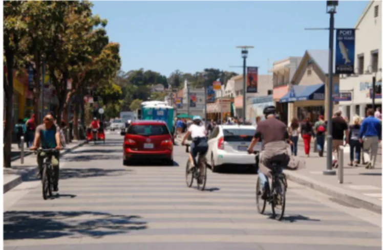
Humans are very proficient in extracting most relevant information from cluttered visual scenes. This is due to the human ability to focus attention on specific targets in a scene and to switch it between different targets rapidly. Suppose you are seeing a common daily scene like the one in Figure 1.1. Initially, you might highlight the more salient elements in the scene, like the red car and ignore the people in the sidewalk or advertisement banners. Such “bottom-up” factors are caused by stimulus saliency and influence the perception of the scene by reflecting sensory inputs. On the other hand, if you are supposed to find your friend in the crowd, you might very well ignore the cars and bicycles and search for the people in the sidewalk in a finer detail. During this process, ones cognitive state enhances the targets percept by modulating the neural responses in various areas of the brain. These “top-down” factors, refine neural responses to serve the requirements of the current and future goals to optimize the processing in order to do the planned task [12]. In everyday life, visual perception is mediated by a mixture of bottom-up and top-down factors and understanding the governing dynamics of this interaction plays an important role in our understanding of the visual perception process. In the following sections, the process of visual perception and its attentional modulations will be introduced. We will focus specifically on attentional modulation of semantic representations across the human brain during search for object categories, the main topic of study in this thesis.
Figure 1.1: Visual perception
of a cluttered scene.
Vi-sual perception is mediated by both “bottom-up” factors, re-flecting the salient stimulus fea-tures, and “top-down” factors, addressing the requirements of processing the cognitive state. (photo courtesy: Aaron Bialick)
1.1
Visual perception
“The eye is like a mirror, and the visible object is like the thing
re-flected in the mirror.” – Avicenna, early 11th century
Since ancient times, eye was believed to be the organ enabling us to “see” the world. But it was only after Kepler at seventeenth century that image reflection on the retina became widely accepted as the major mean of vision. Our under-standing of the vision process has grown from then on. One of the major means of interpreting surrounding environment is processing the information in visible light. At the first step of the process of visual perception, illumination and color of the image is captured by photoreceptors. Photoreceptors are specialized cells on the retina that are sensitive to various properties of light. This information is projected through the optic nerve to the most posterior area of the cortex known as the lower visual cortex. Lower visual cortex is divided into multiple func-tional and anatomically segregated areas [34]. First area involved in early visual processing is the primary visual cortex (also known as V1). Neurons in V1 are sensitive to simple image features. Single-neuron experiments have revealed that different types of neurons in V1 respond to bars with various angles and to bars moving in various directions [34]. There is also a well-defined spatial mapping of the visual field in V1 [56].
Second major visual processing area in the cortex is the prestriate cortex (also known as secondary visual cortex or V2). Neurons in V2 respond to more com-plex features such as orientation and illusionary contours which are particularly important in visual association [34]. An important function of V2 is that it helps identify whether a piece of visual stimuli is part of an object or not, and to seg-regate objects from background [24]. V2 neurons receive strong connections from V1 and send strong connections to V3 and V4. V3 (also known as the third visual complex) is known to be an important cortical area enabling one to have a perception of depth [60]. V4 (also known as the fourth visual complex) is widely known for its role in processing orientation, spatial frequency and color, similar to V2 but in a much more complex manner. In particular, high selectivity to color is a major functional difference between V4 and V2. V4 also plays role in perception of geometric shapes [46]. There are multiple studies suggesting that visual processing is divided into two main paths beyond V4 [26, 23].
Ventral pathway (the “what” pathway) consisting of V4 and extends to inferior temporal cortex (IT). Cortical areas in the “what” pathway play a major role in perception of objects within visual scenes. Inferio-temporal cortex includes vari-ous functional sub-regions, among which are FFA, PPA, EBA and LO. Fusiform face area (FFA) located on the ventral surface of the temporal lobe, responds strongly to faces. The idea of a specific cortical region responsive to faces was
first introduced by Kanwisher et al. [35]. Generally, FFA is localized as voxels1
in lateral side of fusiform gyrus which show significant increased response while subjects view images of faces versus while they see images of general objects. Parahippocampal place area (PPA) is a part of the parahippocampal cortex that resides in medial inferior temporal cortex. PPA was first introduced by Epstein and Kanwisher [21] as a cortical area selective for scenery. PPA is localized to vox-els in the parahippocampal cortex, significantly responding to images of scenery versus images of general objects. Extrastriate body area (EBA) is an area selec-tive for human body parts. EBA is located in the lateral occipitotemporal cortex and is localized as voxels which show significant response to human body parts versus images of general objects [17]. There is also an area in the lateral occipital
1The term “voxel” used throughout this thesis is the short hand form of “volumetric pixel”,
cortex (LO) which strongly responds to general objects with a clear 3D shape [37]. The object-selective area LO, is commonly localized to voxels in lateral occipital cortex that show significant response to images of objects versus scrambled tex-ture images. A major observation regarding the selectivity of the cortical areas along ventral stream is that the complexity of the information processed by the neurons increases as we go from retinotopic areas toward object-selective regions. The dorsal stream (the “where” pathway) appears to have the role of processing visual motion and visual control of attention. The main dorsal cortical area known to be responsive to moving stimuli is MT area, located in the middle temporal lobe. It sends strong connections to intraparietal sulcus (IPS) and to areas in prefrontal cortex, such as frontal eye field (FEF) and frontal operculum (FO). These areas are believed to function in controlling saccadic eye movements and producing top-down attentional modulating signals [40, 41], thus they are known as part of an attention-control network.
1.2
Attentional modulations of visual
percep-tion
Attention plays a crucial role in dedicating the limited resources of the brain in a way to process the cognitive demands and the external triggers. According to the goal of attention, it may be categorized into “spatial attention”, “feature-based attention” and “object-based attention”.
Various single-cell studies have revealed different aspects of neuronal activity en-hancements due to attention. Prinzmetal et al. [49] have reported that observers detect faint stimuli better if the stimuli appear at an attended location. This is the consequence of both lowered neural firing threshold (i.e. enhanced sensitivity) and increased firing rate as a result of spatial attention. These observations are reported in various single cell studies [53, 52] and are consistent throughout the visual system [61, 55].
Cognitive enhancements of covert attention (i.e. directing spatial attention with-out changing the direction of gaze) are characterized as enhancing visual sensi-tivity and reducing reaction times. A recent study by Pestilli and Carrasco [48] showed that covert cued attention to the left or right of a fixation point enhances sensitivity to a flashing object presented for a small period of time. That is, subjects were more successful at correctly identifying presence of a flashing tar-get in either side of the fixation point, if it was preceded by a directional cue shown at the fixation point. In another cognitive experiment, Prinzmetal et al. [49] had presented flashing stimuli in two sides of the fixation point and recorded reaction time in detecting a target, with and without presence of a spatial cue in the fixation point, employing the recording from a button pressed by subject if he detects the target. They have shown that reaction times are lowered if the flashing stimuli is preceded by a spatial cue. Top-down modulations also rise from object-based attention. For example, attending to humans in a scene trig-gers neural activations in attention-control cortical areas which in turn modulate the activation in cortical areas selective for humans in favor of processing human features [55].
1.2.1
Semantic representation of scenes and its
atten-tional modulation
Humans are able to perceive thousands of distinct object and action categories in visual scenes. So it is highly unlikely that each category be represented in an individual area in the cortex. A recent study has proposed that a wide range of actions and object categories are represented in a low-dimensional semantic space across the cortex [31]. Using an experiment in which subjects passively viewed natural movies while their brain activity was recorded using fMRI, Huth et al. [31] have showed that object categories are embedded in a four-dimensional semantic space, shared across subjects. They state that semantically similar categories are projected close to each other and semantically different categories are projected to distinct locations on the cortex. It is also shown that attention to an object category, warps semantic representation across the cortex in favor of the
attended target by expanding its representation across cortex [9]. According to these studies, representation of object categories that are semantically related to the target are also expanded. This suggests that attention dynamically modulates cortical representation in favor of the processing of behaviorally relevant objects during natural vision.
1.2.2
Different accounts for divided attention
Behavioral effects of attending to multiple items has been a subject of debate in recent years. A large body of studies from both neuro-imaging and single cell perspectives have reported that task performance is decreased when the number of items to be attended are increased [44, 45, 20]. In other words, when the observer is about to pick the target among distractors, it takes more time, and the selection error rate across trials is increased as the number of items present on the screen increases [44]. There are mainly two theories presented to account for this lowering in performance.
According to “decision integration model”, quality of representation for each item is not affected as the number of attended items increase, but rather the divided attention results in an increase in the error rate in target detection [20]. This account assumes that the observer has noisy representations of all of the tar-gets and distractors and considers the attention mechanism as a target detection task [58]. In this view, each item in the field of view elicits an internal response in the observer plus a random internal noise due to uncertainty in the neuronal activity. Because of this internal noise, the observer might misidentify a distrac-tor as the target, resulting in a decrease in detection performance and an increase in reaction time [58]. By running experiments in which human subjects searched for an ellipse with multiple different features (i.e. color, orientation, size) among multiple other ellipses, Palmer [44] developed a model that succeeds in showing the predictions of the decision integration model using signal detection theory.
On the other hand, the perceptual coding (also known as ”biased competi-tion”) hypothesis assumes that since the brain has limited computational power,
dividing attention between multiple objects limits perceptual resources and their representation quality is lowered compared to when each of them are the sole search target [19]. The biased competition theory is based on three main princi-ples. First, representation of visual information in different visual systems (sen-sory and motor, cortical and subcortical) in the brain is “competitive”. Second, this competition is “controlled” meaning that it can be biased in favor of one the multiple competing stimuli. Third, the competition is retained across systems. If some portion of the stimulus gains dominance in one system (e.g. early visual cortex) it will retain its dominance in other systems (e.g. higher order visual areas) as well [4].
Several neuro-imaging studies have based their findings on the ground of biased-competition paradigm [36, 57, 51, 14, 38, 3, 2]. Beck and Kastner [2] have studied the effect of attention to Gabor patches with specific orientations among multiple patches with different orientations. Their findings suggest that neurons in early visual areas evoke less response when multiple items appear simultaneously, as a sign for the divided attention being “competitive”. They propose that this effect is more prominent as we go from lower to higher stages of visual processing (i.e. from V1 to V4). There is also strong evidence stating that origin of the top-down signals altering the bias in the biased competition are areas outside visual cortex, including IPS, FEF, SEF and FO [7, 30, 12].
One recent study by Reddy et al. [51] has assessed the biased-competition the-ory using BOLD responses recorded while subjects viewed static images of iso-lated objects and attended to either a single object category among four possible choices (faces, houses, shoes, cars), or two categories simultaneously. A multi-voxel pattern analysis on BOLD responses recorded in category-selective areas in ventral-temporal cortex suggested that response patterns elicited during divided attention to a pair of categories can be expressed as a weighted combination of the response patterns elicited during attention to each constituent category alone. In PPA and FFA, the weights for this combination showed a significant bias to-wards the preferred object category [51]. These results can be taken to imply that category-selective regions in ventral-temporal cortex retain highly modular representations of preferred categories under divided attention. In another study, Reddy and Kanwisher [50] were able to decode object categories present in the
visual stimuli, from the cortical BOLD responses in FFA and PPA in various clutter levels and in the presence of divided attention. This shows that represen-tation of the preferred object categories in object-selective areas FFA and PPA, is robust in presence of clutter and diverted attention.
In this thesis we investigated the effects of divided attention on semantic rep-resentation across the human brain. We hypothesized that divided attention among multiple categories modulates semantic representation in accordance with the biased-competition theory. We recorded whole-brain BOLD responses while subjects viewed a diverse selection of natural movies and performed category-based search tasks. In the divided-attention task subjects searched for “humans” and “vehicles”, and in the two isolated-attention tasks they searched for “hu-mans” and for “vehicles” individually. We used a voxel-wise modeling framework to measure category-tuning profiles of single voxels in each individual subject and under each attention condition [42]. We then evaluated the biased-competition theory by testing two key predictions. First, we asked whether semantic-tuning profile of a voxel during divided attention can be expressed as a weighted average of semantic-tuning profiles during the two isolated-attention conditions. We then asked whether the weights for this linear weighted average show significant bias towards a preferred category in regions across ventral-temporal cortex.
In chapter 2 we introduce some basic concepts needed for the general reader to have a grasp on the materials provided throughout the thesis, including the exper-imental methods, analytical basis and practical considerations taken to reach the results. Chapter 3 includes the results derived from the study and a discussion following the conclusion of the results is provided in chapter 4.
Chapter 2
Materials and Methods
2.1
Behavioral task
There have been many studies of visual attention using still images or simple stimuli like moving bars. Although these simple stimuli provide valuable insight into basic properties of visual perception, they lack the complexity of the visual stimuli human beings encounter in daily life. Another problem in experiments with simple stimuli is that the position of stimuli is usually known beforehand. Although some studies have used random positions for placing the stimuli in the receptive field they still lack the generality of the cluttered natural scenes in which multiple objects appear in various locations in the visual field. In this thesis we have used natural movie clips including a diverse set of objects under clutter and in various contexts to overcome the limitations of the above mentioned simplified experimental paradigms.
Subjects viewed a continuous, color natural movie compiled from 10-20 second clips extracted from Google, YouTube videos. A broad range of indoor and outdoor scenes including 831 object and action categories were present in the clips. The stimulus was separated into three 8-minute-long blocks, and each block was shown in a separate run. Subjects performed three separate visual-search tasks while viewing the same movie stimulus: visual search for “humans”, visual
search for “vehicles”, and visual search for both “humans” and “vehicles”. The experiment was performed in a total of 9 runs and the search task was interleaved across runs. To ensure subject vigilance, subjects were asked to respond with a button press whenever a target was present in the stimulus. Button-press responses were analyzed to ensure that the subjects were performing the search task and to assess any major difference in task difficulties.
2.2
Data collection
2.2.1
Subjects
Five human subjects (four males and one female) have participated in the ex-periment. The experimental data analyzed in this thesis was collected at the University of California, Berkeley.
2.2.2
Recording the brain activity
Functional magnetic resonance imaging (fMRI) is a noninvasive modality to assess neural activity in the brain, indirectly through changes in blood flow and blood oxygenation using magnetic resonance imaging (MRI). When a neural population in the brain gets activated, blood circulation and the amount of oxygen in the blood in the activated area increases. The protein responsible for transporting oxygen in the blood is Hemoglobin. Magnetic properties of Hemoglobin change when it gets oxygenated. It is diamagnetic when oxygenated but gets paramag-netic when deoxygenated. Thus, fluctuations in the oxygenation level in a brain area is related to minor changes in its magnetic properties. These fluctuations in magnetic properties lead to small changes (typically not more than 4 percent [54]) in the MR signal which is measured as a proxy for neuronal activity. This signal is generally called the blood oxygenation level dependent (BOLD) signal.
2.2.2.1 Hemodynamic Response
The BOLD signal is sensitive to the local cerebral blood flow, the rate of oxygen consumption by the activated neurons (also known as “cerebral metabolic rate of oxygen”), and the local cerebral blood volume [8]. The overall effect of these factors that relate the neuronal activity with BOLD signal is often called the hemodynamic response. The BOLD signal lags neural activation by 1-2 seconds and have a temporal width of 5-6 seconds. It commonly ends with an undershoot [8].
Buxton et al. [8] have proposed a simple computational model which explains dynamics of the BOLD signal change, reflecting the undergoing physiological pro-cesses. A simplified description of the model which relates BOLD signal change
to local blood volume (Vact
V0 ) and oxygenation(
Eact
E0 ) changes can be expressed as
∆S S0 ≈ C. ! 1 − Vact V0 (Eact E0 )β " (2.1) in which ∆S
S0 is the MR signal modulation, C is a locally constant scaling term
and β lumps the effects of the MR scanner magnetic fields. The aforementioned dynamics of the BOLD signal is due to the varying dynamics of local blood vol-ume and oxygenation during the aftermath of the neural activation.
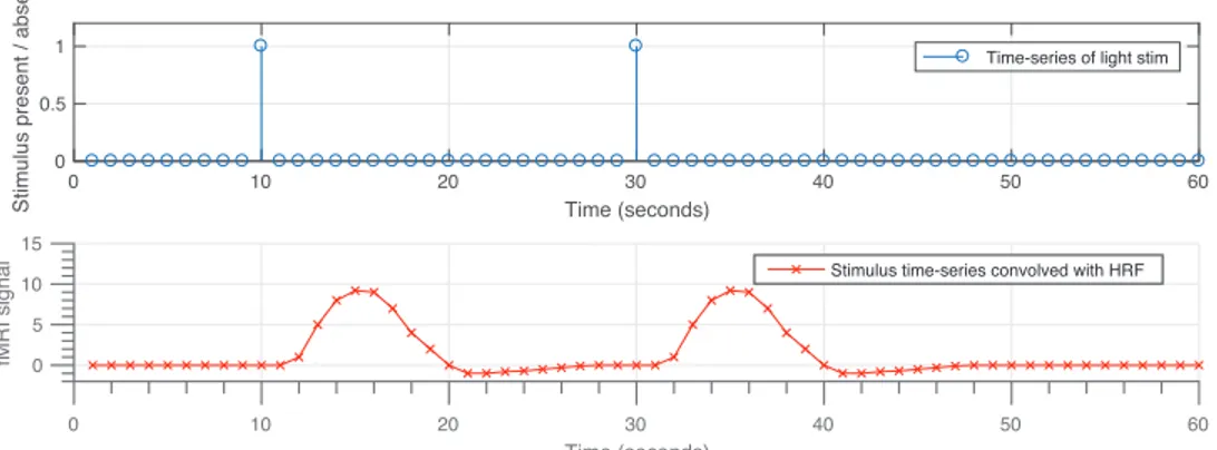
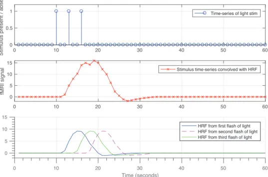
Figure 2.1 illustrates the shape of a typical hemodynamic response function (HRF). The HRF resulting from two separate brief stimuli results in the plot in Figure 2.2 in which two consequent peaks are the result of convolving the HRF with the sequence of stimuli. In fact, HRF functions as a low-pass filter, smoothing the underlying neuronal firings, thus, it limits the temporal resolution of the recorded BOLD signal. This effect is illustrated in Figure 2.3. To avoid unnecessary complexities, we have modeled the hemodynamic response using an FIR filter, which will be discussed in later sections.
In this study, we used functional MRI to measure brain activity while subjects performed the requested tasks. MRI data were assessed on a 3T Siemens scanner located at the University of California, Berkeley using a 32-channel receiver coil. Functional data were acquired using a T2*-weighted gradient-echo EPI pulse se-quence using the following parameters: repetition time(TR) = 2s, echo time(TE)
0 5 10 15 20 Time (seconds) -2 0 2 4 6 8 10 fMR I si g n a l
Figure 2.1: Typical shape of the hemodynamic response
filter. Hemodynamic response
incorporates a time lag in the output, beside the smoothing it produces due to its limited fre-quency width. 0 10 20 30 40 50 60 Time (seconds) 0 0.5 1 St imu lu s p re se n t / a b se n t
Time-series of light stim
0 10 20 30 40 50 60 Time (seconds) 0 5 10 15 fM R I si g n a
l Stimulus time-series convolved with HRF
Figure 2.2: Hemodynamic response resulting from two consecutive brief stimuli. Hemodynamic response filter smooths out the high-frequency content of the input and incorporates delays. This results in two slow varying peaks recorded using fMRI.
0 10 20 30 40 50 60 0 0.5 1 St imu lu s p re se n t / a b se n t
Time-series of light stim
0 10 20 30 40 50 60 0 5 10 15 fM R I si g n a
l Stimulus time-series convolved with HRF
0 10 20 30 40 50 60 Time (seconds) 0 5 10 15 fM R I si g n a
l HRF from first flash of light
HRF from second flash of light HRF from third flash of light
Figure 2.3: Hemodynamic response leads to limited temporal resolution in BOLD response. Due to low-pass filtering effect of the HRF, neural firings resulting from closely presented stimuli are represented as a single peak in the BOLD signal, this leads to limited temporal resolution of the recorded BOLD signal.
= 34ms, flip angle = 74◦, voxel size = 2.24 × 2.24 × 3.5 mm3, field of view = 224
× 224 mm2
. 32 axial slices were acquired to cover the entire cortex. To create cortical flat maps we used a three-dimensional T1-weighted MP-RAGE sequence
to collect anatomical data with 1 × 1 × 1 mm3
voxel size and 256 × 212 × 256
mm3
field of view.
2.3
Data preprocessing
A collection of steps need to be performed in order to make an fMRI BOLD response ready for analysis. The preprocessing steps employed in this study are motion correction, compensation for low frequency drifts and brain tissue extraction.
2.3.1
Motion correction
Motion correction (also known as “realignment”) is a process to correct the head motion effects on the acquired functional data. Even slight head movements cause voxel displacements and changes the signal received from a voxel, reducing the quality of the data. Motion correction tries to correct the movements by aligning different image frames across the fMRI series to a reference volume image, using a rigid body affine transformation. The reference image could be any single image in the series, or the mean image of the series. Head movements are characterized by six variables, three translation parameters, corresponding to linear translation in three Cartesian axes, and three rotation parameters, corresponding to amount of rotation around the three axes. Motion correction in this study was performed using the tools in SPM12 package (http://www.fil.ion.ucl.ac.uk/spm/), and using the first image frame as the reference in each session. Motion correction might lead to flips or sudden rotations of the brain tissue in some cases. Thus, to ensure the validity of realignment, motion-corrected time series was inspected manually for any flaws in each session separately.
2.3.2
De-trending
There are low frequency drifts present in the BOLD signal due to physiological activity (e.g. respiration and cardiac activities). There are also slow drifts due to the scanner warming and eddy currents which incorporate modulations in MRI scanner magnetic fields during the experiment. To compensate for these effects, we filtered the fMRI time series using a second order Savitzky-Golay filter with 120 second window. De-trended responses for each voxel were then z-scored to attain zero mean and unit variance.
2.3.3
Brain extraction
fMRI provides us a 3D image of the brain activation in each time instance, but it includes other tissues such as skull as well. So the brain tissue should be segmented out before moving further. There are various tools used in neuroscience studies for segmentation and extraction of the brain tissue. We used “brain extraction tool (Bet)” from FSL 5.0 package for this purpose [32]. As the result of the brain extraction, we ended up with roughly 50000 to 80000 brain voxels for the subjects of this study.
2.4
Functional regions of interest
Functional regions of interest (ROIs) are generally identified using “localizer” scans to identify voxels in specific anatomical areas showing a particular response (as described in section 1.1). The ROIs of study are determined as the cortical voxels which show significance in the localizer scans plus a neighborhood of voxels in their 2mm vicinity in depth of the brain. Broad ROI boundaries were drawn on the cortical flat maps. Because of the differences in signal-to-noise-ratio values of recorded fMRI data among individual subjects, the broad regions of interest were shrunk to include only voxels having contrast response above half of maximum
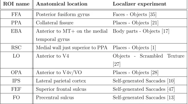
response across cortex in each subject individually. Lastly, voxels in the 2mm depth vicinity of shrunk cortical ROI voxels were included. Table 2.4 summarizes the localizer experiments used to identify each ROI.
ROI name Anatomical location Localizer experiment
FFA Posterior fusiform gyrus Faces - Objects [35]
PPA Collateral fissure Places - Objects [21]
EBA Anterior to MT+ on the medial
temporal gyrus
Body parts - Objects [17]
RSC Medial wall just superior to PPA Places - Objects [1]
LO Anterior to V4 Objects - Scrambled Texture
[27]
OPA Anterior to V4v/VO Places - Objects [28]
IPS Lateral parietal cortex Self-generated Saccades [10]
FEF Superior frontal sulcus Self-generated Saccades [47]
FO Precentral sulcus Self-generated Saccades [13]
Table 2.1: Functional ROI locations and localizers. Functional ROIs studied in this thesis were identified using localizer scans performed independently of the main experiment.
Localizer experiments for category-selective areas were performed in six 4.5min runs of 16 blocks. In each block, subjects passively viewed 20 static images randomly selected from one of the “objects”, “scenes”, “faces”, “body parts” and “spatially scrambled objects” for a total of 16 seconds [27]. Sample images used in localizer scans is shown in Figure 2.4. Each image was shown for 300ms following a 500ms blank. To localize attention-control areas, one 10min run of 30 blocks was used. Either a self-generated saccade, in which the subject was asked to follow a target pattern, or a blank period was prescribed in each 20sec block [10].
body parts faces objects places scrambled objects
Figure 2.4: Sample images used in localizer scans. To localize
category-selective areas, 20 static images randomly selected from one of the “objects”, “scenes”, “faces”, “body parts” and “spatially scrambled objects” were shown for a total of 16 seconds in each block.
2.5
Voxel-wise modeling
2.5.1
Category model
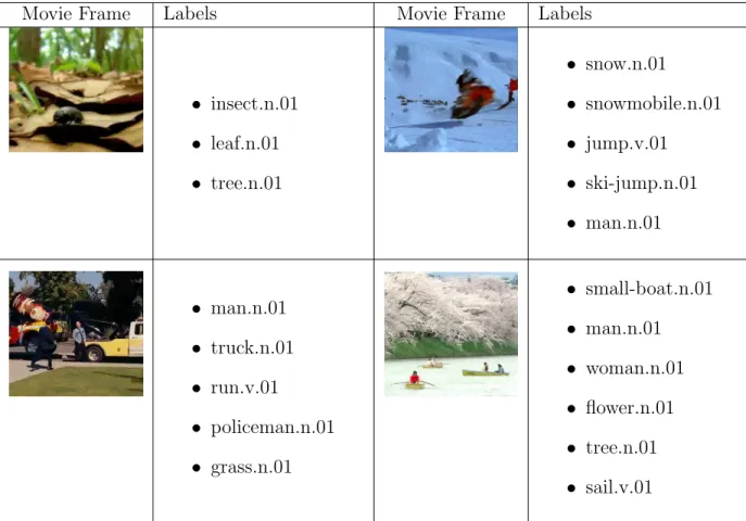
A voxel-wise model was fit to the data to describes the contribution of differ-ent object and action categories to the recorded BOLD activity [9]. Each one second of the clips were labeled for the presence of objects (i.e. nouns) and ac-tions (i.e. verbs) in them, using a collection of terms present in the WordNet lexicon [39]. WordNet is a set of hierarchical directed graphs assigning semantic relationships among words. For example, “entity → person → child” is a branch in the WordNet graph, indicating that a “child” is a “person” and thereby an “entity”. Presence of superordinate categories were also inferred using the hier-archical relations (e.g. whenever a “man” is present, a “human” is also present). Different labeled movie frames are shown in Table 2.2. Using labeled frames, a “stimulus matrix” was built and filled with binary elements, in which each ele-ment represents the presence of the corresponding category in the corresponding time instance in the movie clip. Procedure details are explained in Chapter 2. The stimulus matrix was temporally down-sampled by a factor of two to match
the sampling rate of the fMRI scans.
Movie Frame Labels Movie Frame Labels
• insect.n.01 • leaf.n.01 • tree.n.01 • snow.n.01 • snowmobile.n.01 • jump.v.01 • ski-jump.n.01 • man.n.01 • man.n.01 • truck.n.01 • run.v.01 • policeman.n.01 • grass.n.01 • small-boat.n.01 • man.n.01 • woman.n.01 • flower.n.01 • tree.n.01 • sail.v.01
Table 2.2: Labeling movie frames for presence of object and action
cat-egories. Each one second frame of the movie clip was labeled using the words
from WordNet lexicon providing a total of 831 object and action categories. Cat-egories were then used to construct the stimulus matrix.
2.6
Hemodynamic response
Recalling that what we measure as the BOLD response is an aftermath of neural firings rather than direct neural activity, the hemodynamic response of the brain that maps neural activity to the BOLD signal should be taken into account. To consider the delay resulting from the hemodynamic response, we concatenated 4, 6 and 8 seconds delayed stimulus vectors. Under this scheme, these vectors indicate
presence of categories four, six and eight seconds earlier. This is equivalent to convolution of the stimulus matrix with a three-tap finite impulse response filter.
2.7
Nuisance regressors
2.7.1
Head-motion and physiological noise
Although passing the data through preprocessing steps prunes it for some of the high-frequency noise and slow drifts, we further compensated for residual physiological-noise and head-motion effects by regressing out nuisance regressors. The cardiac and respiratory activity were collected using a pulse oximeter and a pneumatic belt during the runs. They was used to estimate two regressors to capture respiration and nine regressors to account for cardiac activity [59]. Affine motion parameters estimated from momentarily head motions during the motion-correction preprocessing stage were taken as the head-motion regressors. The collection of these regressors were used to regress out the head-motion and physiological-noise modulations from the BOLD responses.
2.7.2
Motion energy correlation
To account for spurious correlation between motion-energy and object-action cat-egories in the natural movies, a nuisance regressor that describes the total motion energy during each one-second of the movie clip was employed as described in [42]. This regressor was formed by taking the mean energy across each one second frame of the movie clip, calculated by applying multiple Gabor filters with differ-ent oridiffer-entation and scales to the frame. The Gabor filter bank consisted of several stages of filtering and transformation. First stage comprised of transforming the stimuli into the International Commission on Illumination LAB color space and removing the color channel, retaining the luminance information. Luminance
channel was then passed through 6555 spatiotemporal Gabor filters with differ-ent scales, oridiffer-entations and spatial and temporal frequencies. At last, the Gabor motion-energy was assessed by squaring and summing outputs of quadrature fil-ter pairs, and the results passed through a logarithm compressive nonlinearity and temporally down-sampled to the fMRI acquisition rate [42]. The resulting time series was taken as the motion-energy regressor.
2.8
Category weights
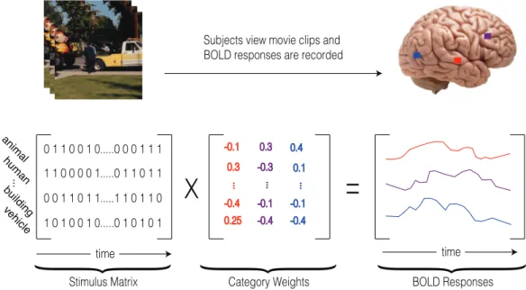
Category weights were assessed using regularized ridge regression (also known as “Tikhonov Regularization”) of stimulus matrix and the recorded voxel-wise BOLD signals. Figure 2.5 illustrates the process of assessing category weights. The optimal regularization parameter for each voxel was picked by doing a 20-fold cross validation. In each fold, data was randomly split such that 90 percent of time samples were used to find weights using different regularization parameters
in the range λi = [1, 10 × 220] and the Pearsons correlation coefficient of predicted
and recorded BOLD responses in the remaining 10 percent of samples was taken as the prediction score. Cross-validation was performed for each of the candidate
regularization parameters (λi) and the regularization parameter that maximizes
the mean prediction score across 20 folds was picked as the optimal value (see Appendix A). After picking the optimal regularization parameter for each voxel, voxel-wise category weights can be assessed by solving the equation:
ˆ
wi = (STS+ ΓTΓ)−1STri (2.2)
in which S is the stimulus matrix containing time series of presence of each category in rows, Γ is the diagonal matrix containing voxels-wise optimal
regu-larization parameters, ri is the matrix containing voxel-wise BOLD response in
rows and ˆwi is the matrix of voxel-wise category weight vectors for i = H, V, B
indicating “attend to humans” (H condition), “attend to vehicles” (V condition) and “attend to both humans and vehicles” (B condition). Category weight ma-trices assessed in this modeling framework describe the contribution of each of the object and action categories to the voxel BOLD responses.
x
=
time anima l huma n ve hicle building ... 0 1 1 0 0 1 0...0 0 0 1 1 1 1 1 0 0 0 0 1...0 1 1 0 1 1 0 0 1 1 0 1 1...1 1 0 1 1 0 1 0 1 0 0 1 0...0 1 0 1 0 1 time{
{
{
Stimulus Matrix Category Weights BOLD Responses
Subjects view movie clips and BOLD responses are recorded
Figure 2.5: General procedure of obtaining model weights. Voxel-wise cat-egory weights were assessed using regularized ridge regression of stimulus matrix and voxel-wise BOLD responses. Each element in the category weight matrix accounts for the contribution of an specific category in the voxel BOLD response.
2.8.1
Target detection effect
To account for spurious correlation between BOLD response and target detection, a target regressor was used indicating the presence of the target in each one-second frame of the movie stimulus. This target regressor was equivalent to the “human” category regressor for the search for “humans” task, and to the “vehicle” category regressor for the search for “vehicles” task. For the divided attention task, the target regressor was taken as the union of the binary “human” and “vehicle” category regressors. To regress out effects of target detection from BOLD responses, the stimulus matrices were aggregated across the three search tasks, and model fits were performed on this aggregated stimulus matrix (Figure 2.6). Using the aggregated stimulus and response matrices, the model can be
described as Sagr = # diag(S, S, S) T $ (2.3) T =% sH sH ⊕ sV sV & (2.4) Ragr = ⎡ ⎢ ⎢ ⎣ rH rB rV ⎤ ⎥ ⎥ ⎦ (2.5) ˆ Wagr = ⎡ ⎢ ⎢ ⎣ ˆ wH ˆ wB ˆ wV ⎤ ⎥ ⎥ ⎦ = (ST
agrSagr+ ΓTΓ)−1SagrT Ragr (2.6)
in which sH and sV are the rows from the stimulus matrix S corresponding to the
“human” and the “vehicle” categories respectively and ⊕ performs the binary OR
operation. rH, rV and rB are the BOLD responses collected in the three search
tasks and ˆWagr stores the model weights for the search tasks.
2.9
Projection onto semantic space
To estimate a semantic space of category representation, principal components analysis (PCA) was performed on voxel-wise category weights in each subject. Principal components analysis projects voxel category weights (category-tuning vectors) onto a space in which data points are uncorrelated. Thus, semantically similar categories are projected to nearby points in the semantic space, and the categories with less semantic similarity are projected to distant points. To avoid overfitting, we performed PCA on the model weights pooled across the two single-target attention conditions. Due to existence of multiply many object categories that humans can perceive, the real semantic representation underlying category tuning profiles in the brain is high-dimensional. Thus, the collection of principal components (PCs) that explain at least 90 percent of the variance in the data were selected for further analysis in each subject. This gave between 36 to 47 principal components for the five subjects. Semantic-tuning profiles were then
{
Category Weights Attend “humans” Attend “both” Attend “vehicles” time voxels{
Aggregated BOLD Responses animal human vehicle building ... 0 1 1 1 0...0 0 1 1 1 1 0 0 1...0 1 1 1 0 0 1 1 1...1 1 1 0 1 0 1 0 0...0 1 0 1
=
x
0 1 1 1 0...0 0 1 1 1 1 0 0 1...0 1 1 1 0 0 1 1 1...1 1 1 0 1 0 1 0 0...0 1 0 1 0 1 1 1 0...0 0 1 1 1 1 0 0 1...0 1 1 1 0 0 1 1 1...1 1 1 0 1 0 1 0 0...0 1 0 1 0 0 0 0 0...0 0 0 0 0 0 0 0 0...0 0 0 0 0 0 0 0 0...0 0 0 0 0 0 0 0 0...0 0 0 0 0 0 0 0 0...0 0 0 0 0 0 0 0 0...0 0 0 0 0 0 0 0 0...0 0 0 0 0 0 0 0 0...0 0 0 0 0 0 0 0 0...0 0 0 0 0 0 0 0 0...0 0 0 0 0 0 0 0 0...0 0 0 0 0 0 0 0 0...0 0 0 0 0 0 0 0 0...0 0 0 0 0 0 0 0 0...0 0 0 0 0 0 0 0 0...0 0 0 0 0 0 0 0 0...0 0 0 0 0 0 0 0 0...0 0 0 0 0 0 0 0 0...0 0 0 0 0 0 0 0 0...0 0 0 0 0 0 0 0 0...0 0 0 0 0 0 0 0 0...0 0 0 0 0 0 0 0 0...0 0 0 0 0 0 0 0 0...0 0 0 0 0 0 0 0 0...0 0 0 0 1 1 0 0 1...0 1 1 1 1 1 1 0 1...0 1 1 1 1 0 1 0 0...0 1 0 1{
Aggregated Stimulus MatrixSubjects view movie clips and BOLD responses are recorded
target
Figure 2.6: Control for target detection effects. To account for the possible modulation of BOLD responses by target detection, a target regressor was added to the model. Target regressor was equivalent to the “human” regressor for the “search for humans” task, the “vehicle” regressor for the “search for vehicles” task and the binary union of the “humans” and the “vehicle” regressors for the “search for both humans and vehicles” task. By populating the aggregated cat-egory model, model fitting was performed simultaneously for the three attention conditions and target detection effects were regressed out of the BOLD responses.
obtained by projecting category models for each task onto the semantic space defined by these PCs.
2.10
Linearity analysis
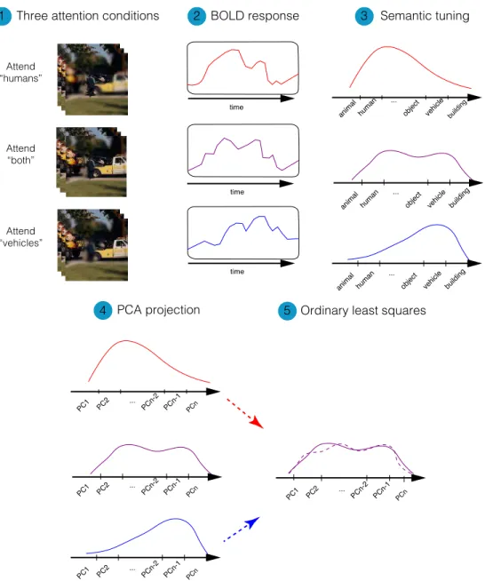
We tested whether the semantic-tuning profile during divided attention can be described as a weighted average of the semantic-tuning profiles during single-target tasks. We performed an ordinary least-squares analysis among semantic-tuning profiles in three attention conditions to linearly describe the semantic-tuning profile in divided-attention condition using tuning profiles in the single-target attention conditions. The problem can be formulated as
wPB = [1 wPH wPV] ⎡ ⎢ ⎢ ⎣ β1 β2 β1 ⎤ ⎥ ⎥ ⎦ = XB (2.7)
in which wPB, wPH and wPV are the voxel-wise semantic tuning profiles for the
B condition, H condition and V condition respectively. Regression weights β1 ,
β2 and β3 can be assessed by solving the equation
ˆ
B = (XTX)−1XTw
PB (2.8)
and a prediction of wPB results from
ˆ
wPB = X ˆB (2.9)
We took the Pearsons correlation between predicted and actual
semantic-tuning profiles in divided attention condition (wPB), as the voxel-wise linearity
index. Figure 2.7 illustrates the procedure of obtaining the linearity index. Higher linearity index means that the tuning profiles in divided attention
con-time
time
time
animal human object vehicle building
...
animal human object vehicle building
...
animal human object vehicle building
... PC1 PC2 PCn-2 PCn-1 PCn ... PC1 PC2 PCn-2 PCn-1 PCn ... PC1 PC2 PCn-2 PCn-1 PCn ... PC1 PC2 PCn-2 PCn-1 PCn ... BOLD response
Three attention conditions 2 3
1 Attend “humans” Attend “both” Attend “vehicles”
PCA projection 5 Ordinary least squares
4
Semantic tuning
Figure 2.7: Linearity index calculation procedure. Voxel-wise linearity in-dex was measured based on the correlation of the predicted and actual semantic tuning profile in divided attention condition (B condition). Tuning in B condi-tion was predicted using an ordinary least-square on tuning profiles in attend to “humans” (H condition) and attend to “vehicles” (V condition). Dashed lines indicate predicted and solid line indicates measured tuning profiles. Thus, the linearity index indicates the accuracy in linear prediction of semantic-tuning pro-files of divided attention condition using semantic-tuning propro-files in the isolated attention conditions.
dition can be better described as a weighted average of tuning profiles in isolated attention conditions.
2.11
Category weight shift analysis
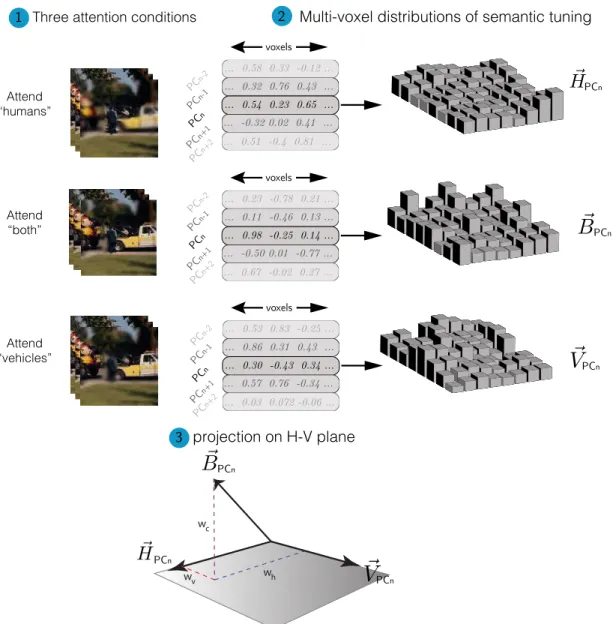
We have hypothesized that the weights in the weighted average are biased towards the preferred object category in object-selective cortical areas. To put this hy-pothesis into test quantitatively, multi-voxel distribution of semantic tuning was examined. Specifically, the tuning distribution during divided attention was re-gressed onto the tuning distributions during the two single-target tasks. We then computed a shift index to measure the direction and magnitude of attentional bias in semantic tuning. The procedure is illustrated in Figure 2.8. In this analy-sis, we projected the semantic-tuning pattern during divided attention condition onto the hyperplane defined by the tuning distributions during the single-target attention conditions. This projection was performed via ordinary least-squares.
Projections were obtained by solving the problem stated in Equation 2.10 using ordinary least squares:
⃗
B = whHˆ + wvVˆ + wc (2.10)
in which ˆV and ˆH are the unit vectors in the direction of ⃗V and ⃗H respectively
(see Figure 2.8). wh, wv and wc are are the regression weights indicating the
contribution of ⃗V and ⃗H in the linear combination respectively.
We quantified a normalized “Shift Index” as
SI = wh− wv
|wh| + |wv|
(2.11) Positive SI values means that the tuning distribution during divided attention is biased towards the distribution in the attend to “humans” condition and neg-ative values indicate bias towards the distribution in the attend to “vehicles” condition.
... 0.58 0.33 -0.12 ... ... 0.51 -0.4 0.81 ... ... 0.32 0.76 0.43 ... ... -0.32 0.02 0.41 ... ... 0.54 0.23 0.65 ... PCn PCn-1 PCn-2 PCn+1 PCn+2 voxels ... 0.23 -0.78 0.21 ... ... 0.67 -0.02 0.27 ... ... 0.11 -0.46 0.13 ... ... -0.50 0.01 -0.77 ... ... 0.98 -0.25 0.14 ... voxels PCn PCn-1 PCn-2 PCn+1 PCn+2 ... 0.53 0.83 -0.25 ... ... 0.03 0.072 -0.06 ... ... 0.86 0.31 0.43 ... ... 0.57 0.76 -0.34 ... ... 0.30 -0.43 0.34 ... voxels PCn PCn-1 PCn-2 PCn+1 PCn+2
1 Three attention conditions 2 Multi-voxel distributions of semantic tuning
3 projection on H-V plane PCn PCn PCn PCn PCn PCn w h w v w c Attend “humans” Attend “both” Attend “vehicles”
Figure 2.8: Shift index calculation procedure. Semantic tuning profile dis-tribution during divided attention was regressed onto the tuning disdis-tributions during the two single-target tasks. Regression weights determine the bias in tun-ing distribution durtun-ing divided attention towards any of the tuntun-ing distributions in the single-target attention tasks. Shift index is then calculated using the re-gression weights to quantify the bias.
Chapter 3
Results
3.1
Experiment difficulty and subject vigilance
The results of the button press task show that subjects were successful in detect-ing targets with rates 91%, 90% and 82% in the “search for humans”, “search for vehicles” and “search for both humans and vehicles” tasks. Successful hit-rate for attend to “humans”, to “vehicles” and to “both” tasks were 0.90 ± 0.10, 0.90 ± 0.09 and 0.82 ± 0.11 respectively. There were no significant differences (one-way ANOVA, F (2) = 1.01, p = 0.3919) in the correct hit rates for the three search tasks. This result ensures that following results are not a mere consequence of difference in experiment difficulty.
Attend “Humans” Attend “Vehicles” Attend “Both”
Figure 3.1: Behavioral per-formance under different
at-tention conditions.
Per-formance of behavioral task (i.e. button press task) is calculated for the three attention condi-tions. Error bars represent stan-dard error of the mean across five subjects. There were no sig-nificant differences in the cor-rect hit rates for the three search tasks.
3.2
Category model performance
In order to make conclusions using the assessed category weights, the underlying category model should have a reasonable accuracy.
After picking the optimal voxel-wise regularization parameters, nuisance regres-sors described in section 2.7 were removed from the stimulus matrix and voxel-wise models were fit. Voxel-voxel-wise BOLD responses were then predicted using the estimated category weights. Performance of the category model fit in each voxel was quantified by the Pearson’s correlation between predicted and actual BOLD responses.
Figure 3.2 shows the prediction score on cortical flat maps for the five subjects of study. Flat maps are produced using Pycortex [25] software package. Voxels that appear in bright yellow have high prediction scores and the models are not significant in gray areas (t-test, p > 0.05 FDR corrected). The ROI boundaries on the maps are drawn by specifying boundaries on contrast maps, gathered from localizer scans. It is seen that the category model predicts fairly well in most of the dorsal and ventral visual streams.
RH LH superior anterior anterior S1 S2 S3 S4 S5 Prediction Score 0.0 0.25 Figure 3.2: Cortical
flat maps of
pre-diction scores for
the five subjects.
To ensure the validity of the category model used across the study,
prediction score of
the category model
is illustrated on the cortical flat map for
the five
subjects(S1-S5). Prediction scores
were quantified as the
Pearson’s correlation
between the predicted and measured BOLD
responses. Brighter
regions have higher
prediction score and
darker areas have lower prediction score. Model
predictions are not
significant in gray areas (t-test, p > 0.05 FDR
corrected). The
corti-cal regions identified
from localizer sessions’ data are drawn and labeled on the maps. Voxels across much of the dorsal and ventral visual streams are well predicted.