The Behavior of Stock Returns in Turkey; 1986 - 1988
A Thesis
Submitted to the Department of Management
and the Graduate School of Business Administration of Bilkent University
in Partial Fulfillment of the Requirements for the Degree of
Master of Business Administration
by
ERDEM BASÇI
I certify that I have read this thesis and in my opinion it is fully adequate in scope and in quality, as a thesis for the degree of Master of Business Administration.
Dr. Kürsat Avdogan
I certify that I have read this thesis and in my opinion it is fully adequate in scope and in quality, as a thesis for the degree of Master of Business Administration.
'S
prof. Sübidev Togan
I certify that I have read this thesis and in my opinion it is fully adequate in scope and quality, as a thesis for the degree of Master of Bussiness Administration.
Approved by the Graduate School of Business Administration
A B S T R A C T
Thef B€tha:uioi- o j S t o c k . Ftot'o.rn& i n T u r k o y : 1986 - 1988
ERDEM BASÇI MBA in Ma.nageinen t
Supervisor: Assist.Prof. Kursat Aydogan September 1989, 120 pages
This study investigates distributional and time series behavior of common stock returns in Istanbul Stock Exchange (ISE) for the period 1986-1988. The distributions of weekly price returns deviate from normality with sharp peaks, heavy tails and positive skewness. These observations are similar to those of United States stock markets but ISE returns have higher means and higher variances. The first order serial dependence is insignificant for most stocks and Box-Jenkins linear forecasting models shows a poor performance. So, published past price information cannot be used to obtain better forecasts of future prices by this model. This observation is in line with the random walk behavior as expected from a weak form efficient market. Applicability of Box-Jenkins models may be questioned however, since variance of returns is not stationary due to a second order dependence. This type of dependence is not against weak form efficiency and is seen in US stock returns as well. To detect any longer term dependence, the test of variance-time function is employed.:· The results indicate significant long term dependence for most stocks and this is against weak form efficiency. The weekly change in trading volume series turns out to be forecastable by univariate Box- Jenkins models and it seems to explain some of the variation in stock price returns.
Keywords: Market efficiency, random walk behavior, Box-Jenkins ARIMA models, stationärity, test of variance time function.
Ö Z E T
T ü ı: k i y e ' d e H i £: s e S e n e d i G e t i r :i 1 c-: r i n i n D a v r a n ı ç ] : ]986 - 1988
ERDEM BAÇÇI
Yüksek Lisans Tezi, içletme Enstitüsü Tez Yöneticisi: Yd.Dop.Di'. Küx*.f:at Aydoğ'an
Eylül 1989, 120 sayfa
Bu çalışma i.stanbul Menkul Kıymetler Borsası'ndaki hi.sse senedi getirilerinin olasılık dağılımları ve zaman içindeki davranışlarını incelemektedir. Haftalık getirilerin dağılımı sivrilik ve çarpıklık açılarından normal dağılımdan farklılık göstermektedir. Bu gözlem gelişmiş hisse senedi piya.salar ındaki lere benzemektedir ancak İMKB getirilerinin ortalama ve varyansları daha yüksektir. incelenen senetlerin çoğu için birinci derece dizisel bağımlılık anlamlı bulunmamış, ve Box- .Jenkins dogıusal kestirira modelleri başarılı olamamıştır. Dolayısıyla yayınlanmış geçmiş fiyat bilgisi gelecekteki fiyatların bu modelle tahmininde bir iyileşme sağlayamaz. Bu
yuruyuş modellerinin bu gözlem zayıf tür etkin bir piyasadan beklenen
davrai'üş lyla tutarlıdır. A,nca.k Box-Jenkins
dizilere uygunluğu sorgulanabilir, çünkü getirilerin varyansı ikinci derece bir bagınılılık dolayısıyla durağan değildir. ikinci derece bağa iiıl 11 j k , zayaf etkinliğe aykırı olmayap gelişmiş piyasalarda da görülmektedir. Daha uzun dönemli bir bağımlılığın varlığı ise varyans-zaman fce.sti ile sınanmaştır. Sonuçlar senetlerin bir kısmı için anlanılı bir uzun dönem bagımlıî ığ'an varlığını göstermektedir ve l.'U ra;ssal yürüyüş modeline aykarıdır. haftalık toplam işlem hacmindeki değişim oicnr dizisi Eox-uenkins modelleri ile kestirilebilir bulunmuştur ve bu değişkenin fiyat değişimlerini bir ölçüde açıkladığı göz ien."iiş t ir .
Pazar etkinliği, ras.sa] Jenkin.s AKIMA modelleri, zaili an testi .
yürüyüş ıiiodeli, Box- durağan1ık,
varyans-A C K N O W L E D G E M E N T S
I would like to express my gratitute to Dr. Kür§at Aydogan for his invaluable supervision during the development of this thesis. I also would like to express my thanks to the Management Department of Bilkent University for providing me with the necessary background through the MBA programme. Special thanks go to Professor Subidey Togan for his enthusiastic encouragement and to Dr. Omit Erol for useful comments and suggestions on methodology and interpretation of results. I would like to thank to the Research Department of the Capital Market Board and especially to Mr. Abdullah Akytiz and Mr. Güven Sak for very informative discussions. Also I express my gratitute to the National Productivity Center for the financial support they provided for the project.
TABLE OF CONTENTS Abstract Özet Acknowledgements Table of Contents List of Tables List of Figures 1 ii iii iv vi vi I. Introduction 1
II. A Review of Literature 5
A. Unconditional Distributions of Stock Returns 5 B. Time Series Models and Serial Correlation 8 C. Volatility of Daily Returns and Conditional
Heteroscedastic Models 10
D. Longer Term Behavior and the Test of Variance-Time
Function 13
III. The Case for Turkey 15
A. Istanbul Securities Exchange and Operation of
the Market fo:.v Common Stocks 15
B. The Data 20
C. Unconditional Distributions of Stock Returns 21 1. Summary Statistics
2. Deviations from Normality
D. Intertemporal Dependence of Stock Returns 28 1. Autocorrelation Analysis
2. Box-Jenkins Univariate Models ajid Forecasting Performance
3. Changing Variance and Its Implications
4. A Variance-Time Test for Longer Term Dependence
E. Trading Volume and Its Effects on Re'-urn Series 38 1. Univariate Time Series Analysis of Trade Volume
IV. Results & Conclusions List of References
Appendices
A. Results of K-S Test for Normality
B. Statistics for Four Week Rate of Return on the index
C. Estimated Autocorrelations for Weekly Returns D. Box-Jenkins ARIMA Models
E. ARIMA Modelling Procedure for Selected Series F. For 3 Years Separately Estimated Autocorrelations G. Estimated Autocorrelations for Squared and Absolute
Weekly Returns
H. Analysis of the IMKB-index
I. Analysis of Weekly Total Trading Volume
J. Estimated Cross Correlation Coefficients Between Elate of Changes in Trading Volume and Index
45 49 A1 B1 C1-C15 D1-D2 E1-E16 F1-F6 G1-G15 H1-H5 11-14 J1 41
25. Ti.niç, Seha M. and West, Richard R., 1 979. I r^ves ı ı n f Irı. S e c ’s i ı i l e s : Ej/ı.cıer>i Harkets Approach, Addison-Wesley
Pub'iishig Company.
26. Unvan, Hayal, 1989. Fı ra r: s a l V a r l ı k l a r L Fvyaiiaridı.rrnc H o d o l ı vo 1 whix'S· Ü'Zo t'ltio B i r Dop.ofiıo: îy /B~iyh’o , Ankara; Sermaye Piyasası Kurulu Yayınları-Yayın No: 11,
27. Young, William E, 1971, "Random Walk of Stock Prices: A Test of the Variance-Time Function", Econornetr i c a ,
LIST OF TABLES Table 1. Table 2. Table 3. Tables 4-9. TalDle 10. Table 11. Table 12. Table 13. Table 14. Table 15. Table 16. Table 17
Frequency of Trading for First Market Stocks
on January 1986 IG
Frequency of Trading for First Market Stocks
on January 1989 17
Developments in Trading Activity of ISE 18 Suirmjary Statistics for Weekly Returns 22-25 Comparison of Weekly Average and Standard
Deviation of Returns 26
Lags of Significant Sample Autocorrelations 29 Diagnostic Checks of ARMA Models 30 Comparison of Forecasting Performances of
Naive and ARIMA Models 32
Were the Means and Variances Equal for Three
Years 34
Number of Stocks for Which Ob.served Variance of m-sum Series Was Greater or Less than the
Estimated Random Walk Variance 36 Number of Stocks with Significant Negative or
Positive Serial Long Term Dependence at the
1% and 5% levels 37
Regression Models 1,2,3 39-40
LIST OF FIGURES
Figure 1. Monthly Trading Volume (198B-198Ö) Figure 2. Weekly IMKB-Index (1986-1988)
19 19
I. INTRODUCTION
The market for common stocks constitutes an important part of the capital market. Besides being the basic source of long term equity financing for corporations, it can provide even very short term investment opportunities for individual investors. Two basic properties are to be expected from an effectively operating stock market. First, it should be developed enough so that any individual investor can purchase "large" amount of securities in a short time without affecting prices, and any firm can raise the necessary funds in a short time from the market. Secondly, the market should be efficient.
Efficiency basicly is related to the health of prices generated in the market. If the price of a security at any time instant can be used as the best estimate of its value, given the set of available relevant information, pricing or external efficiency is said to exist. Operational efficiency on the other hand is used to describe the efficiency of intermediaries in the market. A1locational efficiency is the term used to describe the market that has both pricing and operational efficiency.^ In an allocational 1y efficient market, the price signals of common
stocks will reflect the performance of firms and the health of investment decisions, so resource flow to new investments will be healthy.
As an attempt to promote the development of capital markets in Turkey, Istanbul Securities Exchange has been founded and has started its operations on January 1986. There has been a few studies in an attempt to test the Capital Asset Pricing Model
2
(CAPM) in this market . CAPM basicly assumes existance of arbitrage activity (i.e. buy the underpriced, sell the overpriced) between stocks so as to generate "rational" relative prices eliminating the profit opportunity. Pricing efficiency on the other hand, assumes arbitrage activity through time (i.e. buy when cheap, sell when dear type of behavior) to eliminate the systematic profit opportunity. The purpose of this study is to perform some statistical tests as insights to the degree of pricing efficiency in I.S.E. common stock market while providing some description of the price and return generating process for the three year period from January 1986 to December 1988.
Considering published past price behavior as the only relevant information, Random Walk Theory provides the basic model for the price process. It has two axioms; (1) price changes come from some common probability distribution and ( 2 ) each price change is independent from the past changes. The statistical tests of Random Walk Theory are known as Weak Form Efficiency
3
tests, in the literature . The basic reasoning behind this type of price behavior can be the following. There are sufficient number of speculators to make use of any persistent dependence structures so that such structures fade and only explanation for price changes is changes in "value" due to arrival of new information. So, the only valid tests of weak form efficiency can be statistical ones to detect persistent dependence structures.
In part II of this study, the relevant literature is summarized. In part III, some descriptive analysis of 15 I.S.E. common stock data and I.S.E. index is conducted. First the distribution of price returns and deviations from normality is investigated. The weak form efficiency test of the variance-time function [27] is performed. Box-Jenkins’ time series analysis
[8] is also conducted including autocorre 1ation, partial autocorrelation analyses, model fitting and diagnostic checking
for appropriate series. Observations about heteroscedasticity and its implications are stated. Trading volume series is also analyzed both as a univariate series and as an explanatory variable in a dynamic regression model to affect the price index. Results and conclusions are presented in part IV.
II. A REVIEW OF LITERATURE
A.UNCONDITIONAL DISTRIBUTION OF STOCK RETURNS
The possible probability distribution of common stock returns has attracted many researchers to the field. Fama [14,p,41] gives three reasons for the importance of knowing the distribution of stock returns. These are,
. To give an idea of riskiness to the investor,
. To provide descriptive information about the process generating price changes,
. To justify the validity of using statistics like mean and variance as descriptive tools.
Traditionally, a normal distribution for stock returns has been assumed, basicly due to the ease of computations and theoretical justification from the Central Limit Theorem. "If transactions within a time interval are fairly uniformly spread over time and price changes between transactions are independent and identically distributed with finite variance, the only distribution for price change over that interval is "normal"" [1 4,p4 4], Fama, in his 1965 paper, recognizing the fat tails in distribution of daily returns of stocks in Dow Jones Index, proposed a non-normal stable distribution. Stable Paretian, a
genera! class of stable symmetric distribution, has infinite variance and exhibits fat tails for ';v<2 where 1 s the characteristic exponent. If c' = 2 the Stable Paretian reduces to normal and for o'=1 , it becomes Cauchy distribution.
Blattbery & Gonedes in 1974 report that o; is not constant over time [5]. They propose a continous mixture of normal (Gaussian) distributions where variance itself is taken as a random variable. As a specific case, if variance is distributed as inverted Gamma, the posterior distribution reduces to Students-t. They have compared symmetric Stable and Students-t distributions based on Likelihood ratio test which favor Students-t. Also sums of returns (taken by Monte Carlo methods) appear to converge to normality. This is consisteht with "Student" whereas not consistent for "stable" type distributions. So, they conclude that Student model has greater descriptive validity than the symmetric stable model proposed by Fama.
A discrete mixture of Gaussian distributions was proposed by Kon in 1984 [18]. Although it seems to fit the data better, his suggestion has some undesired features. The number of distributions that enter the mixture is introduced as an additional parameter and that number vary with selection of stocks.
A generalized beta distribution of the second kind (GB2) for individual stock returns were introduced and proposed by Bookstraber and McDonald (1987) [7]. A large number of distributions can be obtained as special cases of GB2. Therefore, It can be seen as an unrestricted model and tests based on Maximum Likelihood comparisons of specific models are facilitated by the introduction of this distribution. They have tried to fit the distribution to stock return data and they report moderate success.
Regardless of the study, all authors have reported that observed distributions are leptokurtic, that is they have heavy tails and sharp peaks. Also, nonzero skewness was observed. To model skewness, lognormal distribution [10] and to model fat tails, stable Paretian family were considered. Badrinath and Chatterjee propose g, h, and (gxh) distributions [4]. g is a skewed distribution, h an alonged one and gxh, obtained by multiplying the two, has both skewness and elongation, they claim their method to be of more practical use, since calculations in the estimation process are easier. Hence they recommend the use of gxh distribution in three moment Capital Asset Price Models (CAPM) and the development of four or higher moment criteria CAPM mode 1s .
All the above studies were concerned mainly on the unconditional distributions of returns and the sequence of the
s e n e s were not important. The results, however, are important since they guide selection of appropriate statistics for testing hypothesis, give an idea of the shape of observed distribution, and lead to the separation the concepts of serial independence and serial uncorre1atedness of stock returns due to the non-normality of distributions. Also the fat tails have implications for existence of autocorrelation in the time series data.
B. TIME SERIES BEHAVIOR AND SERIAL CORRELATION
The basic motivation in investigation of stock market returns as time series has arisen from the debate on Efficient Market Hypothesis. Before 1970’s a random walk model was seen as a
4
necessary condition for weak form efficiency, That is the returns were required to be independent and identically distributed. So, tests of serial autocorrelation in return processes were used as indicators to degree of independence. And for some stocks, the first order serial autocorrelation was found to be significant [14]
In his 1970 paper [15], however, Fama recognizes that independent and identical distribution is not necessary for "fair game' efficiency. The process X(t) will be a fair game, and there will be fair game efficiency in P(t) if
where
E(X \0 )=0
1,1+1 I t
X = P -E(P jö ) J,t + 1 J,t.+ 1 J,t + 1 ' t
and 6^: all the information about the history. A special case would be
E(P I Ö ) > P
j,t+l ' l jt
which is called a submartingale (Martingale, if equality holds). So, a martingale process would imply efficiency and any systematic trade rule would not overperform simple buy and hold. Similarly, a "fair game" process, which does not necessiate zero autocorrelation would imply efficiency. Considering the above points, and the low magnitudes of autocorre1 ation, Fama, concludes that no point against efficiency can be made out of that.
But still, some nonlinear dependence may yield existence of' profitable trading rules whose existence is shown by Akgiray (1988) [1] on absolute value of R and where R denotes the daily return series.
Very recently, Conrad and Kaul [11] in line with the "fair game" efficiency model argument of Fama, fit an AR(1) process to expected returns which reduce to an ARMA(1,1) process in terms’of
observed returns. The data is weekly returns of 10 equal weighted portfolios of NewYork and American Stock Exchange common stocks for the period 1962 to 1985. As a result they obtained values of Î varying from .087 to .589. They conclude that $<.6 implies r"apidly decaying time variation in expected returns. So that a shock in expected returns would dissipate after a month. Although they start with the assumption of market efficiency, using their model, an arbitrager would easily overperform simple buy and hold of course neglecting transaction costs.
Oldfield & Jarrow (1977) [19] have proposed an autoregressive jump process for common stock returns, the time intervals between jumps being distributed Gamma. In Perry’s 1982 paper, the null hypothesis of stationary and "independent" increments is rejected [2 0].
C. VOLATILITY IN DAILY RETURNS AND CONDITIONAL HETEROSCEDASTIC MODELS
Although the serial correlation can be modelled by Box Jenkins models, it has been observed that there is second order dependence in residuals which cannot be removed by simple AR
5
transformations. This is due to the nonnormal characteristics of return distributions and of residuals. The AR transformation
eliminates serial correlation in residuals but, the high degrees of autocorrelation observed in absolute and squared residuals even at long lags cannot be eliminated. This is an implication of nonlinearity of the process. That is it cannot be represented as
inear combination of independent and i dentical 1y distributed (white noise) processes and its second moments are
0 not constant over time which indicates nonstationarity
The Autoregressive conditional Heteroscedasticity, ARCH, model introduced by Engle [13] in 1982 and its natural extention Generalized ARCH (GARCH) model introduced by Bollerslev [6] in 1986, are good approximations to type of nonlinearity indicated above. Domowitz has succesfully applied the ARCH model in exchange markets to determine risk premium based on the conditional variance of market forecast errors [12].
For definitions of nonlinearity Priestley [23] p.106 and p.816.
A GARCH process of orders p and q denoted as GARCH(p,q), can be described as follows: X jii FCu ,v ) 1 I i -1 ' I t u = § + •f X ' t o 1 1-1 F· , . 9 “ 1 o .o + E ^ 1 l-v + E^ V=1 J=1 'll X _ ■i - i X " t. t 0 1 1-1
where p>o and q.-o are the orders of the process, and the parameters satisfying conditions a _ > 0, a ,{i. >0 . 0. is the
I I I -1
set of all information available at time t (X ,X . ). When i-1 1-2
q=0, the process reduces to ARCH(p).
Akgiray [1], applied both ARCH and GARCH models to daily stock returns data obtained from CRSP tapes for the period 1963 to 1986. The results obtained were as follows: test statistics supported the use of the models. And the best fit was obtained from a GARCH(1,1) process.
The basic descriptive implication of the models is that large price changes tend to follow large ones and small changes tend to follow small ones. The models can easily be used to forecast volatility and are shown to simulate the ex post (in sample) behavior of stock returns very closely [1]. They can also be used to obtain ex ante measures of variance which can be used for both theoretical and practical purposes.
As long as the deviations from expected returns have zero mean, which is the case for GARCH models, the "fair game
efficiency as introduced by Fama (1 970 ) holds, Hov^ever, the existence of AR(1) coefficient i will be against submartingale
1
behavior. And simple buy and hold strategy will not necessarily be optimal.
D.LONGER TERM BEHAVIOR AND THE TEST OF VARIANCE TIME FUNCTION Looking at the stock returns of longer durations, it is seen that there is a dramatic intertemporal variation. Shiller (1981) [24] questions the validity of EMH. He has calculated the ex-post discounted values of future real dividends to determine a rational price value at a given point in time. Such price series follow a surprisingly smooth path as compared to that of actual price series.
"One is struck by the smoothness and stability of the ex post rational price series Pi' when compared with the actual price
. „ 7 series .
Such a long term dependence even if it exists might escape from the independence tests based on autocorrelation function or number of runs in the same direction. For that reason, different specific tests for long term dependences have been developed and used, Aydogan and Booth [3] for example have used the so called
R/S analysis to detect any long cycles in stock prices from July 1962 to December 1980. They report that long term dependence is either not prevalent or too small to be measured by R/S analysis. Their test statistics, indicate that if long dependence exists, it is positive in the sense that variability at low frequencies is higher than in the high frequencies.
Young [27] has developed a different test based on the variance-time function. The basic idea is that if the returns are strictly independent, the variance of sum of m daily returns should be m times the variance of daily returns. If the variance of the sum is smaller, a negative dependence and if greater, a positive dependence is said to exist. The basic observation of the study is that, for short intervals, for example for m=2,3 and 4, random walk hypothesis of independence cannot be rejected, while for larger values of m, significant deviations from independence mostly negative in direction take place. This dependence leading to price reversals may be the result of the accumulation of weak dependences that are not significant in a short time interval but may accumulate within a longer interval and become more significant. Young notes that this is not completely against the efficient market hypothesis since transaction costs may be the reason for the persistance of such non-random price behaviors.
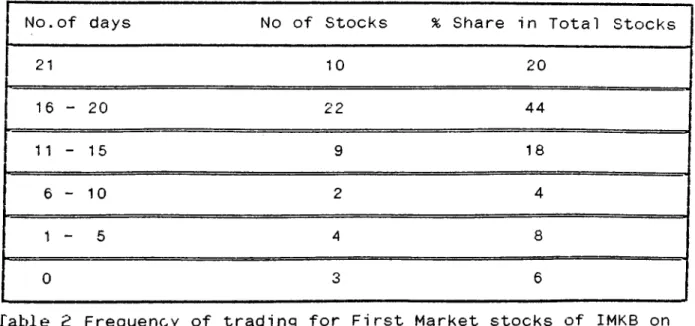
No. of days No of Stocks % Share in Total Stocks 21 10 20 16 - 20 22 44 1 1 - 15 9 18 6 - 10 2 4 1 - 5 4 8 0 3 6
Table 2 Frequency of trading for First Market stocks of IMKB on January 1989
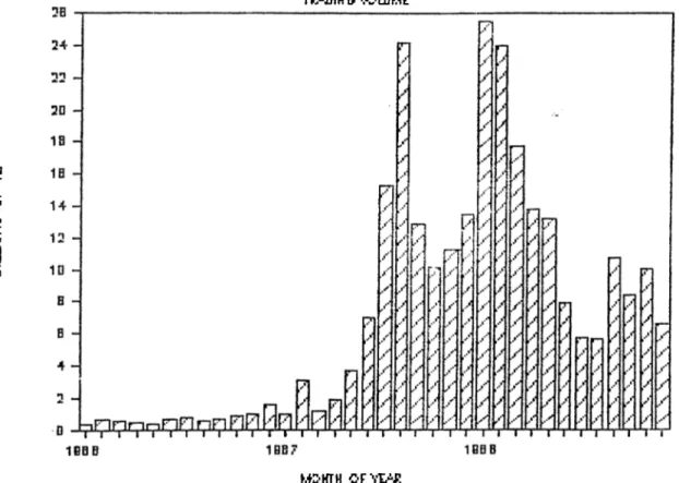
developed stock market. The trading volume should be high enough to enable any individual investor to buy or sell large amount of securities in a very short time period without much affecting prices. For that, trade volume must be large and pricing efficiency must exist. The development of monthly TL trading volume can be seen on figure 1. Although there is a decline in real trading volume in 1988, number of shares traded has increased. As it can be seen from the below table, trading volume has increased by 43.6% while number of shares increased by 115,6%. This is basicly due to the general fall in stock prices
YEAR: 1 986 1987 1 988 Number of shares traded
(Mi 11i ons): 3.2 14.7 31.7
Trading Volume
(Bill ions of T L) : 8.7 105.4 149.0
___________ 1 Table 3: Developments in trading activity of ISE
(Source ISE Annual Bulletins)
after 1987 October. The index calculated and published by ISE, namely the IMKB-index, has fallen from 1140 in July 1987 down to 374 in 1988 end. The plot of IMKB-index for the 3 years is given on figure 2. As it can be seen, up to August 1987, there has been a sharp rise and after August, a decline has taken place up to 1988 end.
The index is calculated according to the formula10
1 40 Pit *Qi t
1= — E * 1 0 0 where,
40 i.=i PiO*Qlo
PLo = Base period price of i stock
• t h
Olo = Base period number of shares outstanding of i stock
t }*i
Pit = Price of i 'stock at period t
Oit = Number of shares outstanding of i stock Pi t ^ Qi t
So, I = _______ is an indicator of the change in total
It
Pi Qi Û
market value of a common stock relative to the base period value
10
I c : ^^4. I ^ I.. I ! Vl r\LJ· I I I i ^L I VI U I i \ ^ L 1R“J3IH C \OLUME IL D V> 5 3 m h+S’KTH oFvt-ï’i:
F i g u r e 1 Monthly Trading volume (Billion TL)
KC HTMS Cf IBEIEf-lfitia
This index at the same time, is a measure of value for an equally weighted portfolio of 40 stocks formed at the base period. The base period value of each stock is taken as a weighted average of January 1986 prices of that stock. Stock splits are also accounted for by this formula. In the following sections, statistical behaviour of the IMKB-index together with 15 selected stocks will be examined.
B. THE DATA
The data basicly consists of weekly Friday closing prices of 15 stocks and IMKB index. To avoid any problems due to missing observations, the selected stocks are those that have been continuously traded within the 3 year period. In addition, weekly trading volume values are compiled.
The focus of attention will be on the series = ln(P^/P ^ ) ,
where P is the price of the security at week t end. This i
corresponds to continuously compounded price return during period t. It is approximately equal to the arithmetic rate of return a = (P -P )/P for small vaues of R Since stock splits and
t t t -1 t I
right offerings are frequent and at high proportions in Turkey, the adjustment
R = ln(k*P - W ) - ln(P )
l T 1 t * 1 t t ■
11.
where k is the stock split ratio, and W is the net payment per share to obtain the new shares is to be performed 114,p.46]. But it would be the same to adjust the prices for splits and payments first and then perform the log-difference transformation on the adjusted prices. So, all the ex-split prices are multiplied by the split ratio and the net payment is subtracted . The effect of dividends is not considered because dividends are distributed on quite a wide time period and it is not possible to identify the exact ex-dividend price. However, this is not likely to alter the results much since the magnitudes are small compared to market prices and its effect would be seen only on 3 out of 156 observations.
C. UNCONDITIONAL DISTRIBUTIONS OF STOCK RETURNS
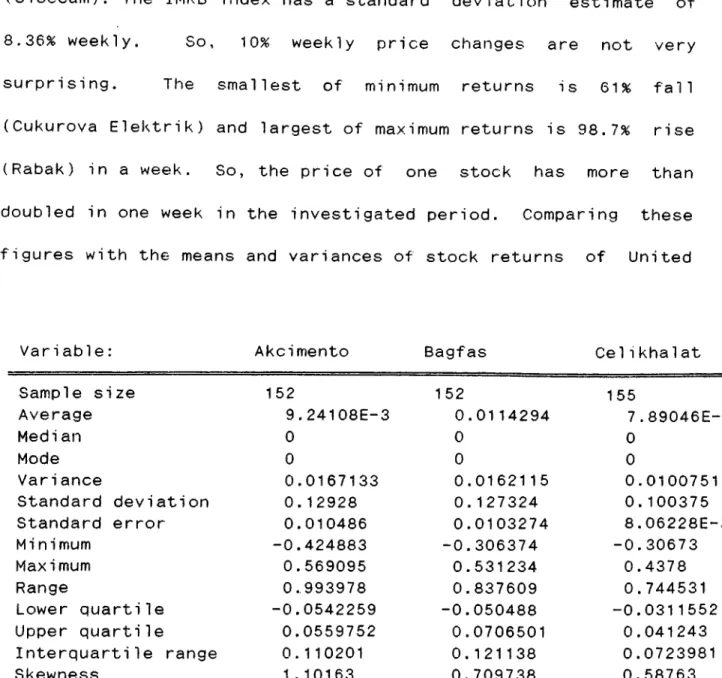
The summary statistics for weekly price returns of 15 stocks and the market index are presented on Tables 4 - 9 . First thing to note is that all the average weekly returns are positive and quite high. The minimum average return was of Celikhalat, by 0.789% weekly, which corresponds to a 41% annual continuously compounded rate and the maximum average return was of Çukurova Elektrik by 1.877% weekly, which corresponds to a 97.6% annual continuously compounded rate. The average for index was 0.85% weekly and 44.2% annual. The next observation is the large variance and standard deviation estimates. Minimum standard
deviation is 9.9% weekly (Kocyatirim) and the maximum is 15% (Sisecam). The IMKB index has a standard deviation estimate of 8.36% weekly. So, 10% weekly price changes are not very surprising. The smallest of minimum returns is 61% fall (Çukurova Elektrik) and largest of maximum returns is 98.7% rise (Rabak) in a week. So, the price of one stock has more than doubled in one week in the investigated period. Comparing these figures with the means and variances of stock returns of United
Variable: Akcimento Bagfas Ce1i kha1 at
Sample size 152 152 155
Average 9.24108E-3 0.0114294 7.89046E-3
Median 0 0 0
Mode 0 0 0
Variance 0.0167133 0.0162115 0.0100751
Standard deviation 0.12928 0.127324 0.100375
Standard error 0.010486 0.0103274 8.06228E-3
Minimum -0.424883 -0.306374 -0.30673 Maximum 0.569095 0.531234 0.4378 Range 0.993978 0.837609 0.744531 Lower quartile -0.0542259 -0.050488 -0.0311552 Upper quartile 0.0559752 0.0706501 0.041243 Interquartile range 0.110201 0.121138 0.0723981 Skewness 1.10163 0.709738 0.58763 „ Standardized skewness 5.54477 3.57227 2.98672 Kurtosi s 4.6719 2.82199 4.37379 Standardized kurtosis 1 1 .7574 7.10184 11.1152
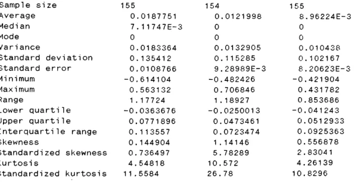
Variable: Cukurova Elk. Erdemi r Kartonsan Sample size 155 154 155 Average 0.0187751 0.0121998 8.96224E-3 Median 7. 1 1 747E-3 0 0 Mode 0 0 0 Variance 0.0183364 0.0132905 0.010438 Standard deviation 0.135412 0.115285 0.102167
Standard error 0.0108766 9.28989E-3 8.20623E-3
Minimum -0.614104 -0.482426 -0.421904 Maximum 0.563132 0.706846 0.431782 Range 1 .1 7724 1.18927 0.853686 Lower quartile -0.0363676 -0.0250013 -0.041243 Upper quartile 0.0771896 0.0473461 0.0512933 Interquartile range 0.113557 0.0723474 0.0925363 Skewness 0.144904 1.14146 0.556878 Standardized skewness 0.736497 5.78289 2.83041 Kurtosi s 4.54818 10.572 4.26139 Standardized kurtosis 11.5584 26.78 10.8296
Table 5 Summary statistics for weekly returns (cont’d)
Variable: Kocyatirim Kordsa Koruma Tarim
Sample size 155 155 155 Average 0.010228 9.90431E-3 0.0109343 Median 0 5.493E-4 0 Mode 0 0 0 Variance 9.90616E-3 0.0120686 0.0125135 Standard deviation 0.0995297 0.109857 0.111864 Standard error 7.99442E-3 8.82393E-3 8.9851 IE-3
Minimum -0.325422 -0.310155 -0.273041 Maximum 0.504436 0.463573 0.563791 Range 0.829858 0.773728 0.836832 Lower quartile -0.0289846 -0.0387145 -0.0357181 Upper quartile 0.0448477 0.0519597 0.0416314 Interquartile range 0.0738323 0.0906743 0.0773495 Skewness 1.09211 0.929463 1.18379 Standardized skewness 5.55082 4.72413 6.0168 Kurtosi s 5.79192 3.91841 5.2321 Standardized kurtosis 14.7192 9.95796 13.2965
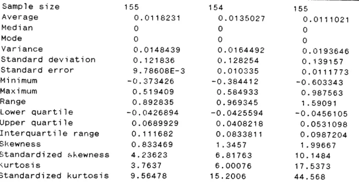
Variable: Lassa Otosan Rabak Sample size 1 55 154 155 Average 0.0118231 0.0135027 0.0111021 Median 0 0 0 Mode 0 0 0 Variance 0.0148439 0.0164492 0.0193646 Standard deviation 0.121836 0.128254 0.139157
Standard error 9.78608E-3 0.010335 0.0111773
Mi nimum -0.373426 -0.384412 -0.603343 Maxi mum 0.519409 0.584933 0.987563 Range 0.892835 0.969345 1.59091 Lower quartile -0.0426894 -0.0425594 -0,0456105 Upper quartile 0.0689929 0.0408218 0.0531098 Interquarti1e range 0.111682 0.0833811 0,0987204 Skewness 0.833469 1.3457 1.99667 Standardized skewness 4.23623 6.81763 10.1484 kurtosis 3.7637 6,00076 17.5373 Standardized kurtosis 9.56478 15.2006 44.568
Table 7 Summary statistics for weekly returns (cont’d)
Variable: Sarkuysan Sisecam Turkdemi rdokum
Sample size 155 154 155
Average 9.72091E-3 8.0724E-3 0.0144562
Median 8.36825E-3 0 0
Mode 0 0 0
Variance 0,0141421 0.022614 0,0106824
Standard deviation 0.11892 0.15038 0.103355
Standard error 9.55192E-3 0.0121179 8.30171E-3
Minimum -0.454736 -0,56453 -0.277632 Max i mum 0.619039 0,834226 0.385056 Range 1.07378 1.39876 0,662688 ■ Lower quartile -0.0327898 -0.0384661 -0.0500104 Upper quartile 0,0512933 0.0425595 0.0707366 Interquartile range 0.0840831 0.0810255 0.120747 Skewness 1.09337 0.859732 0.591371 Standardized skewness 5.55722 4.3556 3.00573 Kurtosis 7.65564 7,90151 1.0597 Standardized kurtosis 19.4555 20.0154 2.69305
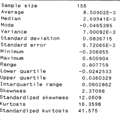
Variable IMKB-index Sample size Average Medi an Mode Variance Standard deviation Standard error Mi nimum Maximum Range Lower quarti1e Upper quartile Interquartile range Skewness Standardized skewness Kurtosi s Standardized kurtpsis 1 55 8.50902E-3 2.69941E-3 -0.0465395 7.00092E-3 0.0836715 6.72066E-3 -0.206855 0.600904 0.807759 -0.0242533 0.0360329 0.0602862 2.37098 12.0509 16.3596 41.575
Table 9 Summary statistics for weekly returns (cont’d)
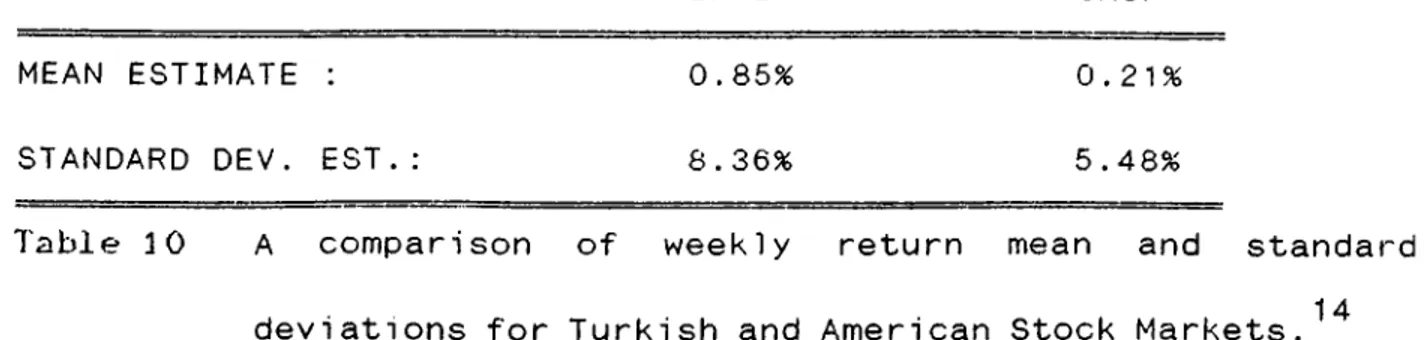
States stock markets, one sees that the ISE is much more Volatile, hence risky but its average returns are larger as Well. Akgiray [1] reports the sample average return of daily
12
CRSP value weighted series for 1963-86 as 0.0422% and the daily variance estimate for the same period as 0.602E-3 The corresponding weekly means and standard deviations are presented on table 10 together with those values of IMKB index just for a
13 compar1 son.
1
2
Center for Research of Security Prices. These indices contain a ’l 1 the stocks of NYSE and AMEX markets.
1 3
INDEX: imp;b CRSP
MEAN ESTIMATE : 0.85%
0
,21
%STANDARD DEV. EST.: 8.36% 5.48%
Table 30 A comparison of weekly return mean and standard 14 deviations for Turkish and American Stock Markets.
The next observation from the summary statistics is that for all series with no exception, median and mode estimates are below the mean estimates. This is an implication for positive skewness 15 of the distribution, The standardized skewness statistics justify this argument. At 95% confidence level, 14 out of 15 stocks and the index are positively skewed (skewed to the right). For the single remaining stock Çukurova Elektrik, median is
14
For the CRSP, weekly mean estimate is five times daily mean estimate and the standard deviation estimate a is calculated
W
2 2 2
from 0 = 5 * a where o is the daily variance. This is only
V d d
approximation. It holds exactly if daily returns are independent.
1 5
Both standardized skewness and kurtosis estimates are distributed approximately Student’s t with degrees of freedom greater than 100.
closer to mean but is still smaller. On the other hand, with no exception, all the 15 stocks and the index turned out to be leptokurtic at 95% confidence level. So they all have sharp peaks and heavy tails as compared to normal distributions. The least leptokutic stock, Turk Demirdokum has a standardized kurtosis measure of 2.69.
To test for normality, Kolmogorov-Smirnov one sample test is employed. This test statistic measures the maximum difference of the observed cummulative distribution from the best fit cummulative normal distribution. If the difference is significant, then the distribution is rejected. The results of the test are presented at appendix A. At 5% significance level, normality is rejected for 14 out of 15 weekly stock returns and at 1% significance level, normality is rejected for 8 out of 15 weekly stock returns.
The distribution of monthly rates of change in IMKB index is also investigated. The summary statistics given at appendix B indicates no skewness and kurtosis at 95% confidence level, and quite interestingly Kolmogorov-Smirnov test fails to reject normality at all significance levels up to 99%. So, although weekly returns are far from normal, monthly returns can be taken as normal quite confidently. This fact makes the suitability of symmetric stable distribution questionable. Sums of returns should also be nonnormal stable under stable laws, which does not
seem to be the case here.
This last observation brings quite a relief since although normality cannot be claimed to exist, means and variances are still defined and can be used as descriptive tools in further analysi s .
D. INTERTEMPORAL DEPENDENCE OF STOCK RETURNS
In a stock market in which prices move as predicted by the random walk theory, the stock return series should be independent and identically distributed. This implies that the theoretical
16
autocorrelation function values pj, should be zero. If the distribution of returns is normal, the sample autocorre1ati on estimates r are approximately normally distributed with mean zero
k
1 7
and variance 1/ T where T is the number of observations. So if the absolute value of a sample autocorrelation estimate r exceeds
k
2/y T , then wi th 96% confidence, p^is different from zero and i s said to be significant. This confidence band is an underestimate for deviations from normality in the form of leptokurtosis.
1
0
The autocorrelation of a stationary series x^at lag k is definedas p = E(x X ) and estimates are calculated as r, = 1/T*rx x
k t t-k k t t-k
Bartlett’s approximation for the case when the series, is completely random [8, p.35].
The sample autocorrelation coefficient plots up to lag 40 together with 2-y confidence bands and coefficient values up to lag 32 with standard errors of estimates are presented at appendix C, The significant spikes are tabulated for the 15 stocks and the index. As it can be seen, for 4 stocks and the index, there are no significant spikes. Only for
Name of Series: Significant Spike at Lag: Akci mentó Bagfas Celi khalat Çukurova Elektrik Erdemi r Kartonsan Kocyati ri m Kordsa Koruma Tarim Lassa Otosan Rabak Sarkuysan Si secam Turkdemi rdokum IMKB-i ndex None 6, 25 6, 18 12, 25 5, 12 6 9 1 , 7, 12, 13, 26 None
1
7, 12 6 None6
,21
None NoneTable 11 Lags of significant sample autocorrelation values for 15 stocks and the IMKB-index
stocks first lag coefficient is significant. For-5 stocks lag 6 coefficient is significant.
18
Provided that the assumptions of stationarity and normality are close approximations, the significant spikes are either
1S.1 wUsed here in distributions.
19 , ...
spurious or they indicate a univariate serial dependence. In the case that the dependence structure is linear, Box-Jenkins
20
univariate ARMA models [8] can be employed for forecasting purposes. Among the 11 stocks with any significant autocorrelation coefficient, 5 stocks with relatively large coefficient values are selected for ARMA model fitting. The identification, estimation, diagnostic checking and model selection phases are presented at appendix E. The summary of the results are given on table 12 below. Constant term is estimated for each model and all are insignificant at 5^ level. The Q
.2
Series Model Tried R Q(20) Selected? Reason
Celi khalat MA(6) 9.1% 14.49 NO
SMA(6) 10.1% 16.57 YES Parsimony
Kordsa AR(1),SAR(7) 9.1% 22.41 NO AR(1),SAR(13) 10.2% 18.34 NO
AR(7) 7.8% 18.39 NO
AR(7),SAR(13) 12.4% 9.51 YES High R^ Low 0 Lassa MA(1 ) 4.8% 19.41 YES High R, Low Q2
AR( 1 ) 3.6% 20.92 NO
Otosan SMA(7 ) 3.9% 20.38 YES Parsimony
Rabak SMA(6) 8.5% 11.82 YES High R, Low Q2
SAR(6) 7.3% 13.19 NO
TABLE 12 Diagnostic Checks of ARMA models
1 9
That means they are realized by chance and have no implication a dependence structure in the series.
The model representation for ARMA models is given at appendix D.
statistics are calculated as the sum of squares of the first 20 autocorrelation estimates of the residual series. Under the
2
hypothesis of uncorre'lated residuals, 0 is distributed n with 20 degrees of freedom. All of the given 0 statistics are insignificant at 10% level. So independence of residuals cannot
2
be rejected. The R values are mean adjusted and the maximum is 12.4% for the AR(7)SAR(13) model of Kordsa. It should be noted that this number is obtained at the expense of parsimony principle.
The diagnostic checks that are tabulated indicate that although not very accurate, the selected models can be used for forecasting purposes. It is interesting however, to note that the models selected for the five series are not similar to each other, while 11 of the 16 series did not require modelling at all. So, it would be wise to see the forecasting performance of the models to check for validity and usefulness. For this purpose, an in sample forecasting was conducted. For each series, the selected ARIMA model forecast errors are compared with the naive forecasts of the martingale model for the last 36
21 ■ '
weeks of 1988 . The comparison is made by the ratio of root mean squared ARIMA model forecast errors to the root mean squared
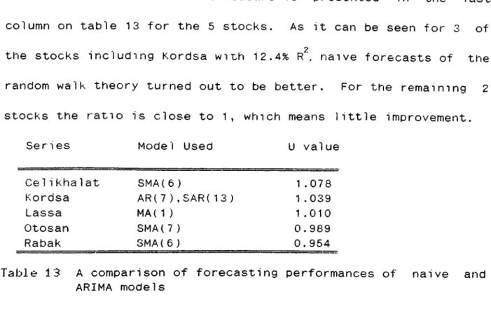
naive forecast errors. This measure is presented in the last column on table 13 for the 5 stocks. As it can be seen for 3 of the stocks including Kordsa with 12.4% R^, naive forecasts of the random walk theory turned out to be better. For the remaining 2 stocks the ratio is close to 1, which means little improvement.
Series Model Used U value
Ce1i kha1 at SMA(6 ) 1.078
Kordsa AR(7),SAR(13) 1 . 039
Lassa MA( 1 ) 1.010
Otosan SMA(7) 0.989
Rabak SMA(6) 0.954
Table 13 A comparison of forecasting performances of naive and ARIMA models
All the above arguments question the usefulness of ARIMA models in forecasting stock prices in IMKB. This may be either due to the nonlinearity of the dependence structure, or due to the nonstationarity of the series. If the nonlinearity is in the form of a second order dependence as reported by Akgiray [1], then the variance is not stationary and the autocorrelation analysis may become meaningless.
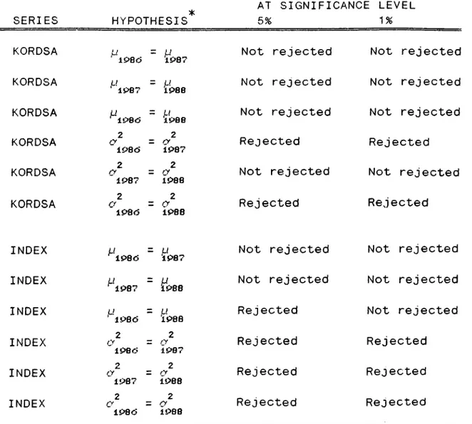
In order to have an idea about stationarity, the equality of distributions of IMKB-index returns for the three years 1986, 1987 and
two sample test based on the differences in the cummulative density functions. At 90% confidence level, paired equality of distributions for the three years is rejected. As a more
detailed analysis of the source of possible non-stationarity, equality of means and variances are compared by the Kolmogorov-Smirnov (K-S) two sample analysis. The results are summarized on table 14 for the IMKB index series and the most problematic series Kordsa. For the both the index return seri es and Kordsa return series, the hypothesis of equal means could not be rejected at 1% significance level. However the hypothesis of equal variances can safely be rejected for all three years with 99% confidence for the index, and it can be rejected for 1986-1987 and 1986-1988 comparisons for Kordsa series. So, one can conclude that the stock return series are not variance stationary. To see how this effects the usefulness of the autocorrelation analysis, the autocorrelation estimates for the three years are plotted seperately for both series at appendix F. The differences between years are remarkable. More interestingly all autocorrelation coefficients are within the confidence band for Kordsa as well as the index. So the huge variance in 1986 has pushed some irrelevant spikes out of the band for the 1986-1988 period.
Given the evidence on nonstationarity of the variance, existence of nonlinear dependence is suspected. To check for any second order dependence, the autocorrelation of absolute and squared returns are plotted and presented at appendix G. For all the series and the index, there is significant first lag positive
autocorre1 ation at the absolute returns. For 14 out of 16 series, there is at least one significant positive spike up to the fifth lag. This is a strong indication of positive second order dependence. It means large price changes tend to follow
large ones and small changes tend to come after small ones. *
SERIES HYPOTHESIS
AT SIGNIFICANCE LEVEL
5 % 1%
KORDSA ¿J
'iPBrj = fJ 1P87 Not rejected Not rejected
KORDSA u
1P87 = iP8B Not rejected Not rejected KORDSA fJ1P8<5 = A1P88·' Not rejected Not rejected KORDSA ry2 1P80-2 = ry 1P87 Rejected Rejected KORDSA 2 1P87 2 = ry
1P88 Not rejected Not rejected KORDSA rr2 ' lP8r> 2 = C> 1P88 Rejected Rejected INDEX A/
lP8rJ = LI 1P87 Not rejected Not rejected
INDEX [J
1P87 = M!IPB8 Not rejected Not rejected
INDEX fJ
lP8d = u1P8B Rejected Not rejected
INDEX O2
1P8C?
2 = (y
iPG7 Rejected Rejected
INDEX cy2 1P87 2 = ry 1PB8 Rejected Rejected INDEX a2 lP8d 2 = ry
IPBB Rejected Rejected
* Two sided tests based on confidence interval for difference
of means including zero and conf. interval for ratio of variances including unity.
It is shown by the above analysis that there is no short term linear dependence structure in weekly returns. The existence of a longer term dependence is checked by the test of variance-time function developed by Young. As discussed in part II-D, if there is no serial dependence, variance of sums of m consequtive returns, should be m times variance of the return series. If the ratio is larger than m, positive, otherwise negative long term dependence is said to exist. To test for the existance of such a phenomena two sample series are necessary for each stock. One is the original return series and the other is the m-sum series. The m-sum series is contructed as a T-m+1 number of overlapping sums of the return series [27,p.806]. Due to its construction, the m-sum series is correlated with the return series. By making use of this property, a test statistic
2 2
for testing the hypothesis a - my where r subscript denotes the
s r
one period return series and s subscript denotes the m-sum or m period return series. If the hypothesized relation holds, the transformation
( 1 ) u = s + m r,
(2 ) V = s - mr;
should generate uncorrelated u and v. So, p =0 can be used as
•J V
an equivalent hypothesis [27,p.805].
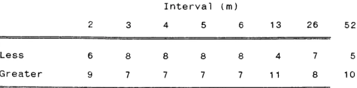
The above procedure is used for the IMKB data. The m values used are { 2,3,4,5,6,12,26,52). Disregarding significance of
observations, table 15 gives the number of series for which observed variance for the ni sum series are greater or less than the estimated return series variance for all the 15 stocks. For
Interval (m)
2 3 4 5 6 1 3 26 52
Less 6 8 8 8 8 4 7 5
Greater 9 7 7 7 7 1 1 8 10
Table 15 Number of stocks for which observed variance of the m 2
sum series (S ) was greater or less than the estimated m
2 random walk variance (mS ).
X
the IMKB-index, the m sum variance was greater than expected for all m values. Up to m=13, the results do not seem to be against the random walk model. At and after m=13 however, the differences seem to be in favor of a positive dependence. Still, all that figure might be a coincidence. To be able to talk more strongly, the statistic mentioned above is calculated for each series. The number of significant p values at 1% and 5% significance levels are presented on table 16 together with the implied direction of dependence. The first observation is that up to m=13 weeks there are only 3 stocks (1 stock only at 1%) which exhibit a long term dependence. For
m=13,26 and 52, at least 6 stocks at 5% (4 stocks at 1%) exhibit significant long term dependence. The interesting point is the change in sign of dependence with the value of m. For m=52,
Leve 1 Type Interval (m)
2 3 4 5 6 13 26 52
Five per cent Negative 0 0 0 2 2 0 3 4
Positive 1 1 1 1 1 6 5 3
One per cent Negative 0 0 0 0 0 0 1 4
Positive 0 1 1 1 1 4 4 2
Table 16 Number of stocks out of 15 with significant negative or positive serial long term dependence at the 5% and 1% level as indicated by ry rna for m=2,3 ,4,5 ,6,13,26,52 week holding period returns 1’·
negati ve dependence is seen more while for m=13 , al 1 the significant dependences are positive . This might imply the existance of local trends which 1 ast almost for 13 weeks and then reverse in direction. Still this is not a very reliable conclusion due to heteroscedasticity. If such a single phenomena has taken place during the high volatility periods, it could cause this observation. But anyway, the statistics do tell the more likely existence of long term dependence as compared to no significant short term dependence.