Decentralized control

(1)

49

Decentralized Control

49. 1 Introduction ... 779

49.2 The Decentralized Control Problem ... 780

49.3 Plant and Feedback Structures ... 781

49.4 Decentralized Stabilization ... 782

Decentralized Inputs and Outputs ° Structural Analysis ° Decentrally Sta-bilizable Structures ' Vector Liapunov Functions 49.5 Optimization ... 785

49.6 Adaptive Decentralized Control ... 787

49.7 Discrete and Sampled—Data Systems ... 788

M. E. Sezer 49.8 Graph—Theoretic Decompositions ... 788

Bilkent University, Ankara, Turkey LBT Decompositions ° Acyclic IO Reachable Decompositions ' Nested Epsilon Decompositions ' Overlapping Decompositions

D. D. Siljak

Santa Clara University, Santa CIara, CA

49.1 Introduction

The complexity and high performance requirements of present-day industrial processes place increasing demands on control technology. The orthodox concept of driving a large system by a central computer has become unattractive for either economic or reliability reasons. New emerging notions are subsystems, in-terconnections, distributed computing, parallel processing, and information constraints, to mention a few. In complex systems, where databases are developed around the plants with distributed sources of data, a need for fast control action in response to local inputs and perturbations dictates the use of distributed (that is, decentralized) information and control structures. The accumulated experience in controlling complex industrial processes suggests three basic reasons for using decentralized con-trol structures: 1. dimensionality, 2. information structure constraints, and 3. uncertainty. Because the amount of computation required to analyze and control a system of large dimension grows faster than its size, it is beneﬁcial to decompose the system into subsystems, and de-sign controls for each subsystem independently based on the local subsystem dynamics and its interconnections. In this way, special structural features of a system can be used to devise feasible and efﬁcient decentralized strategies for solving large control prob-lems previously impractical to solve by “one—shot” centralized methods. 0-8493-8570-9/96/$0.00+$.50 © 1996 by CRC Press, Inc. References ... 791

49.2 The Decentralized Control

Problem

To introduce the decentralized control problem, consider two inverted penduli coupled by a spring as shown in Figure 49.1. The control objective is to keep the penduli in the upright position by applying feedback control via the inputs u] and uz. The linearized equations of motion in the vicinity of 61 = 92 = O are

"18591 - 7602091 - 92) + u1, mg£62 — ka2(62 — 91) + u2. mﬂzél =

mezéz = (49.1)

By choosing the state vector x = (01, 91, 62, 92)T and the input vector u = (u 1 , uz ) T , the state space representation ofthe system is 0 l O O 5_ka2 ka2

5,, =

e

m 0

m

0 x

0 O 0 l k2 k2

_

#27

0 t—m—‘Zf

0-0 0 L 0 + ”‘32 u (49.2) 0 O

1

0 at?

The fundamental restriction in choosing the feedback laws to control the system S is that each input a] and uz can depend only on the local states x1 = (61, 91)T and x2 = (92, 92)T ofthe corresponding penduli, that is, u1 = u1(x1) and u2 = u2(x2). This restriction is called the decentralized information structure constraint.

Since the system S is linear, a natural choice is the linear control laws

u1 = lx1 , u2 = k2Tx2 (49.3)

Figure 49.1 Inverted penduli.

where the feedback gain vectors k1 = (kn, k12)T and k2 = (k21, k22)T should be selected to stabilize the system S, that is, hold the penduli in the upright position.

In control design, it is fruitful to recognize the structure of the system S as an interconnection . 0 1 F0 S:x1 = [a 0]x1+ ﬁ]u1 0 0' 0 o +e[_y 0-161+e[y 0]x2, . 0 1 0 x2 = [a 0]x2+lﬁ]u1 O 0 0 +e[y 0]x1+e[_y ]x2, (49.4) of two subsystems S]: .731 [2 (1)]x1+[2]u1, [2 (1)]x2+ [g]u2,

wherea = g/Z, ,B = l/mZZ, y = dzk/mez, ande = (a/Zz)2. One reason is that, in designing control for interconnected sys-tems, the designer has to account for essential uncertainty in the interconnections among the subsystems. Though models of the subsystems are commonly available with sufﬁcient accuracy, the shape and size of the interconnections cannot be predicted sat-isfactorily either for modeling or operational reasons. In the example, the interconnection parameter e = a /Z1 is the uncer-tain height ofthe spring which is normalized by its nominal value

a.

32: .732 (49.5)

An equally important reason for decomposition is present when controlling large dynamic systems. In complex systems with many variables, most of the variables are weakly coupled, if coupled at all, and the behavior of the overall system is domi-nated by strongly connected variables. Considerable conceptual and numerical simpliﬁcation can be gained by controlling the strongly coupled variables with decentralized control.

(3)

49.3. PLANT AND FEEDBACK STRUCTURES

49.3 Plant and Feedback Structures

Consider a linear constant system

S: x = Ax + Bu,

y

=

Cx,

(49.6)

as an interconnected system

8: ii = Aixi + Biui + Z(A,-jxj + Bijuj) ,

jeN

yi = Cixi + Z Cijxj , i 6N, (49.7)

jeN

which is composed of N subsystems Si: xi = Aixi + Biui,

Yi = Cixi . i e N, (49.8) where x,- (t) E Rm , u ,- (t) 6 Km , y,- (t) 6 Re‘ are the state, input, and output ofthe subsystem S,- at a ﬁxed time t e R. All matrices have proper dimensions, and N = {1, 2, . . . , N}. At present we are interested in disjoint decompositions, that is,

x = (xlT,x2T,...,x17‘;)T,

u = (u{,u{,...,u§,)T, (49.9)

y = (y1T,s.~.,y§)T.

and where x(t) E R", u(t) e Rm, and y(t) 6 Re are the state, input, and output of the overall system S, so that

R" = Rnlazx...xR"N,

Rm = Rm‘ l’"2 x ...mN, (49.10) 1Rz = R31 XRZZX...XR£N.

A compact description of the interconnected system S is 8:12 = ADx + 3011 +ACx + BCu

y

=

CDx+CCx,

(49.11)

where

A1) = diag{A1, A2, . . . , AN},

BD = diag{Bl, Bz, . . . , BN}, (49.12)

CD — diag{C13 C2, ° ' ' s Cl

and the coupling block matrices are

AC = (Aij), BC = (Bij),

CC = (Cij) . (49.13)

The collection of N decoupled subsystems is described by SD:)'C = ADx+BDu

y = Cox . (49.14)

obtained from (49.11) by setting the coupling matrices to zero.

781 Important special classes of interconnected systems are input (BC 2 O) and output (CC = 0) decentralized systems, where inputs and outputs are not shared among the subsystems. Input— output decentralized systems are described as

Szfc = ADx+BDu+ACx

y = CDx, (49.15)

where both BC and CC are zero. This structural feature helps to a great extent when decentralized controllers and estimators are designed for large plants.

A static decentralized state feedback,

u = —KDx, (49.16)

is characterized by a block—diagonal gain matrix,

K1) =diag{K1,K2,...,KN}, (49.17) which implies that each subsystem S; has its individual control law,

ieN,

with a constant gain matrix K). The control law u of (49.16), which is equivalent to the totality of subsystem control laws (49.18), obeys the decentralized information structure constraint requiring that each subsystem S,- is controlled on the basis of its locally available state xi. The closed—loop system is described as

u,- = —K,-x,- , (49.18)

s: 3% = (AD — BDKDCD)x + Acx. (49.19) When dynamic outputfeedback is used under decentralized con-straints, then controllers of the following type are considered:

Ci: 2: = u):

FiZi + Giyi,

—H,-z,- — Kiyi , i e N , (49.20) which can be written in a compact form as a single decentralized controller deﬁned as sz' = FDZ+GDy, u = —HDz—KDy, (49.21) where

z = (zf.z§...z,7&)T.y=(y1T.y2T...y§)T.

u = (ulT,u2T,...,u17(})T, (49.22) are the state z e R', input y 6 Re, and output a e Rm of the controller CD- By combining the system S and the decentralized dynamic controller CD , we get the composite closed—loop system

as

5&c [x] =

Z AD—BDKDCD+AC -BDHD x GDCD FD Z .

(49.23)

(4)

49.4 Decentralized Stabilization

The fundamental problem in decentralized control theory and practice is choosing individual subsystem inputs to stabilize the overall interconnected system. In the previous section, the plant structures have been described, where the plant, inputs and out-puts are all decomposed with each local controller responsible for the corresponding subsystem. While this is the most com-mon situation in practice, it is by no means all inclusive. It is often advantageous, and sometime necessary, to decentralize the inputs and outputs without decomposing the plant. This is the situation that we consider ﬁrst.

49.4.1 Decentralized Inputs and Outputs

Suppose that only the inputs and outputs, but not states, ofsystem S in (49.6) are partitioned as in (49.9), and S is described as

S: X = Ax + Z Eiui, ieN

y,- = éix, i eN. (49.24) Then, the controllers C,- of (49.20) still operate on local measure-ments yi to generate local controls u i: but now they are collec-tively responsible for the whole system. In this case,

. it _ A—BKDC —BHD x

38....[2]_[

F. NJ (49.2.)

It is well—known that without the decentralization constraint on the controller, the closed—loop system of (49.25) can be sta-bilized if, and only if, the uncontrollable or unobservable modes of the open—loop system S are stable; or equivalently, the set of (centralized) ﬁxed modes of S, which is deﬁned as

AC =

ﬂa(A — BKC)

(49.26)

K

is included in the open left half plane, where o(.) denotes the set of eigenvalues of the indicated matrix. This basic result has been extended in [34] to decentralized control of S, where it was shown that the closed—loop system (49.25) can be made stable with suitable choice of the decentralized controllers C,- if, and only if, the set of decentralizedﬁxed modes

AD

=

ﬂaw —BKDC)

KD

= ﬂ 0'(A — Z éiKiéi) (49.27)

K1 ... KN iEN

is included in the open left half plane.

The result of [34] has been followed by extensive research on the following topics:

0 state—space and frequency domain characterization of decentralized ﬁxed modes,

0 development ofvarious techniques for designing de-centralized controllers (e.g. , using static output feed-back in all but one channel, distributing the control effort among channels, sequential stabilization, etc.)

a generalization of the concept of decentralizedﬁxed modes to arbitrary feedback structure constraints, 0 formulation of the concept of structurally ﬁxed

modes, and their algebraic and graph—theoretical characterization.

A useful and simple characterization of decentralized ﬁxed modes was provided in [1]. For any subset I = {i1, . . . , ip} of the index set N, let IC = U], . . . , jN_p} denote the

comple-ment of I in N, and deﬁne

~ BI = [§i,.1§i2,---,l§ipl, (311 .. Cj

CIc

=

,2

(49.28)

CjN—P

Then a complex number A e (C is a decentralizedﬁxed mode of S if, and only if,

rank [A»«_ M BI] < n (49.29)

CIC 0

for some I C N. This result relates decentralizedfixed modes to transmission zeros of the systems (A, 31,file), called the complementary subsystems. Thus, appearance of afixed mode corresponds to a special pole—zero cancellation, which can not be removed by constant decentraliZed feedback. However, under mild conditions, suchfixed modes can be eliminated by time— varying decentralized feedback.

The characterization of decentralized ﬁxed modes above prompts a generalization of the concept to arbitrary feedback structures. Let I? = (EU) be an m x 1 binary matrix such that Eij = 1 if, and only if, a feedback link from output y to input u ,-is allowed. Thus I? speciﬁes a constraint on the feedback struc-ture, a special case of which is decentralized feedback. In this case, permissible controllers have the structure

C12: 2: = FiZi + Z gijyj 1671'

u,- = —h,TZi — Z kijyi (49.30) j€~7i

where (71' = {jtic-ij = 1}.

Let K denote any feedback matrix conforming to the structure of K, that is, one with kij = 0 whenever kij = 0. Then, the set

A]; =

ﬂaw — BKC)

(49.31)

K

can conveniently be defined as the set of fixed modes with respect to the decentralized feedback structure constraint specified by I? . Then the closed—loop system consisting of S and the constrained controller CI? can be stabilized if, and only if, A I? is included in the open left half-plane. Finally, it remains to characterize A I? as in (49.29). This, however, is quite automatic; consider the index setsI C M = {1, 2, . . . , M} and replaceIC byJ = UieICji’ where now IC refers to the complement of I in M.

(5)

49.4. DECENTRALIZED STABILIZATION

49.4.2 Structural Analysis

Structural analysis oflarge scale systems via graph—theoretic con-cepts and methods offers an appealing alternative to quantitative analysis which often faces difﬁculties due to high dimensionality and lack ofexact knowledge ofsystem parameters. Equipped with the powerful tools of graph theory, structural analysis provides valuable information concerning certain qualitative properties of the system under study by practical tests and algorithms [30].

One ofthe earliest problems ofstructural analysis is the graph— theoretic formulation of controllability [20]. Consider an un-controllable pair (A, B). Loss of controllability is either due to a perfect matching of system parameters or due to an incient number of nonzero parameters, indicating a lack of sufﬁ-cient linkage among system variables. In the latter case, the pair (A, B) is structurally uncontrollable in the sense that all pairs having the same structure as (A, B) are uncontrollable. Since the structure of (A, B) can be described by a directed graph (as explained below for a more general case), structural controllabil-ity can be checked by graph—theoretic means. Indeed, (A, B) is structurally controllable if, and only if, the system graph is input reachable (that is, each state variable is affected directly or indi-rectly by at least one input variable), and contains no dilations (that is, no subset of state variables exists whose number exceeds the total number of all state and input variables directly affect-ing these variables). These two conditions are equivalent to the spanning of the system graph by a minimal subgraph, called a cactus, which has a special structure.

The idea of treating controllability in a structural framework has led to formulation and graph—theoretic characterization of structurallyﬁxed modes under constrained feedback [26]. Let D = (V, 5) be a directed graph associated with the system S of (49.6), where V = M U X U y is a set of vertices correspond-ing to inputs, states, and outputs of S, and 8 is a set of directed edges corresponding to nonzero parameters of the system ma-trices A, B, and C. To every nonzero aij, there corresponds an edge from vertex xj to vertex xi, to every nonzero bij, an edge from u1- to x,- , and to every nonzero cij, one from xj to yi. Given a feedback pattern K and adding to D a feedback edge from yj to ui for every kg] = 1, one gets a digraph D1; = (V, 8 U 61?) completely describing the structure of both the system S and the feedback constraint speciﬁed by I? .

Two systems are said to be structurally equivalent if they have the same system graphs. A system S is said to have structurally fixed modes with respect to a given I? if every system structurally equivalent to S hasfixed modes with respect to I? . Having struc-turallyfixed modes is a common property of a class of systems described by the same system graph; if a system has no struc-turallyfixed modes, then either it has no fixed modes, or if it does, arbitrarily small perturbations of system parameters can eliminate thefixed modes. As a result, if a system has no struc-turallyfixed modes with respect to 1?, then genericai‘av it can be stabilized by a constrained controller of the form defined in

(49.30).

It was shown in [26] that a system S has no structurallyﬁxed modes with respect to a feedback pattern E if, and only if

783 1. all state vertices of DI? are covered by vertex disjoint

cycles, and

2. no strong component ofD1? contains only state ver-tices, where a strong component is a maximal sub-graph whose vertices are reachable from each other. This simple graph—theoretic criterion has been used in an al-gorithmic way in problems such as choosing a minimum number of feedback links (or, if each feedback link is associated with a cost, choosing the cheapest feedback pattern) that avoid struc-turallyﬁxed modes. As an example, consider a system with a system graph as in Figure 49.2. Let the costs of setting up feed-back links (dotted lines) from each output to each input be given by a matrix

6 2 3 7 '

It can easily be veriﬁed that any feedback pattern of the form

[i 33]

[’1‘ i],

where >I< stands for either a 0 or a l, avoids structurallyﬁxed modes. Clearly, the feedback patterns which contain the least number of links and which cost the least are, respectively,

- 10 - 01

Kl—[O 0] 01' Kz—[l 0].

Figure 49.2 System graph.

49.4.3 Decentrally Stabilizable Structures

Consider an interconnected system

Aixi + Bi(ui + Z Dijxj)

jeN

S: X; =

y,- = x,- i e N (49.32)

which is a special case of the system S in (49.7) in that Aij = BiDij, Bij = 0, C; = I, and Cij = 0. Assuming that the

(6)

decoupled subsystems described by the pairs (A i, 3,) are con-trollable, it is easy to verify that S has no decentralized ﬁxed modes. Thus S can be stabilized using a decentralized dynamic feedback controller of the form (49.21). However, because the subsystem outputs are the states, there should be no need to use dynamic controllers.

Choose the decentralized constant state feedbacks in (49.18) to place the subsystem poles at —Mil)0, i 6 NJ = 1, 2, . . . , m, where — m; are distinct negative real numbers, and p is a param-eter. Then a suitable change of coordinate frame transforms the closed—loop system of (49.19) into the form

.6»: x = (—pM + Ac)x ,

(49.33)

where M = diag{M1, M2, . . . , MN}, with M,- = diag{/.L1, 11.2, . . , um, }, and Ac is independent of the parameter ,0. Clearly, g is stable for a sufﬁciently large p.

The success of this high—gain decentralized stabilization tech-nique results from the special structure of the interconnections among the subsystems. The interconnections from other subsys-tems affect a particular subsystem in the same way its local input does. This makes it possible to neutralize potentially destabiliz-ing effects of the interconnections by a local state feedback and provide a high degree of stability to the decoupled subsystems. This special interconnection structure is termed the “matching conditions” [18].

Decentralized stabilizability of interconnected systems satis-fying the matching conditions has motivated research in char-acterizing other decentrally stabilizable interconnection struc-tures. Below, another such interconnection structure is de— scribed, where single—input subsystems are considered for con-venience.

Let the interconnected system be described as S: at,- = Aixi +biui + Z Aijxj , i EN

jeN

(49.34)

where, without loss of generality, the subsystem pairs (A), 17,-) are assumed to be in controllable canonical form. For each in— terconnection matrix Aij, deﬁne an integer m ,-j as

if

— : A-- ,

—n, Aij = 0,

Thus, mij is the distance between the main diagonal and a line parallel to the main diagonal which borders all nonzero elements

Of A ij .

For an index set I C N, let Ip denote any permutation of I. Then, the system S in (49.34) is stabilizable by decentralized constant state feedback if

2(mij—1)<O

iel’

jEIP

(49.36)

for allI and all permutations Lo [14] , [30]. In the case of match-ing interconnections, mij = nj — 11,-, so that (49.36) guarantees decentralized stabilizability even when the elements of the inter-connection matrices Aij are bounded nonlinear, time—varying

functions of the state variables. Therefore, the condition (49.36) and, thus, the matching conditions, are indeed structural condi-tions.

49.4.4 Vector Liapunov Functions

A general way to establish the stability of nonlinear intercon-nected systems is to apply the Matrosov-Bellman concept ofvec-tor Liapunov functions [17]. The concept has been developed to provide an efﬁcient method of checking the stability of lin-ear interconnected systems controlled by decentralized feedback [30]. First, each subsystem is stabilized using local state or output feedback. Then, for each stable closed—loop (but decoupled) sub-system, a Liapunov function is chosen using standard methods. These functions are stacked to form a vector of functions, which can then be used to form a single scalar Liapunov function for the overall system. The function establishes stability if we show positivity of the leading principal minors of a constant aggregate matrix whose dimension equals the number of subsystems.

Consider the linear interconnected system of (49.7),

Am + Biui

+Zeiii', iEN, jeN

S: it; =

(49.37)

where the output yi is not included and EU = 0. We inserted the elements of eij e [0, l] of the N x N interconnection matrix E = (eij) to capture the presence of uncertainty in coupling between the subsystems

Si: )5; = Aixi + Biui , (49.38) as illustrated by the example of the two penduli above.

We assume that each pair (A,- , B,- ) is controllable and assign the eigenvalues —af :1: jw‘i, . . . , —O’;;l. :l: jwii, . . . , —021Pi+1’ ..., —a,';i to each closed—loop subsystem

3.; x,- = (A) — BiKi)x,-

(49.39)

by applying decentralized feedback

ui = —K,-x,- .

(49.40)

Using a nonsingular transformation,

x,- = Tiic'i,

(49.41)

we can obtain the closed—loop subsystems as

s, 55, = Ag}, ,

(49.42)

where the matrix A,- = Ti—1(Ai — BiKi)T,- has the diagonal form

diag

1 1-

I."

p'1

1 1 Pi Pi

(49.43)

(7)

49.5. OPTIMIZATION

For each transformed subsystem, there exists a suitable Lia-punov function v: R”" -—> R+ of the form

.. .. .. 4

vi (xi) = (xi Hixi) 2 , (49-44) where H,- = I,- is the solution of the Liapunov matrix equation

AiHi + HiA,‘ = —Gi (49.45) for Gi = diag{0‘1i, of, . . . , all", aim“. . . . , 0,2}.

To determine the stability ofthe overall interconnected closed— loop system ~ .

S: ii = Aiii + Z eiiJ-ij jeN

(49.46)

from the stability of the decoupled closed—loop subsystems 5i, we consider subsystem functions v,- as components of a vector Liapunov function v = (v1, v2, . . . , vN)T, and form a candidate Liapunov function V: R" ——> R+ for the overall system 5 as

VG) = Ediviﬁii),

ieN

(49.47)

where the existence of positive numbers d,- for stability of§ has yet to be established, and Ag = TflAijTj.

Taking the total time derivative of V (56) with respect to 5, after lengthy but straightforward computations [30],

Va) 5 —dTWz, (49.48)

with? = (d1,d2,---,dN)T: z = (llilll, ”552”...” IliN||)T,

and W = (131'j) is the N x N aggregate matrix deﬁned as

' — l 2 . .

_

444—494(454»,z=4

wij = _ 1/2 T . .

”'eijA-M (Aiij), ‘75]

where 0,; is the minimal value ofall a]: , and A M ( - ) is the maximal eigenvalue of the indicated matrix.

The elements éij of the fundamental interconnection matrix E = (égj) are binary numbers deﬁned as

- l,

eij = O

In this way, the binary matrix describes the basic interconnection structure of the system S. In the case of two penduli,

(49.49)

81- acts on

S,-Sj does not act on Si . (49.50)

(49.51)

It has been shown in [30] that stability of —W (all eigenvalues of —W have negative real parts) implies stability of the closed— loop system S and, hence, 8. To explain this fact, we note ﬁrst that wig > 0, wij 5 0 (i 76 j), which makes W an M—matrix (e.g., [30]) if, and only if, there exists a positive vector d (di > O, i e N), so that the vector

J = dTW

(49.52)

is a positive vector as well. Positivity of c and d imply V(5c') > O and V(5E) < O and, therefore, stability of S by the standard

785 Liapunov argument. Finally, the M—matrix property of W is equivalent to stability of — W.

Several comments are in order. First, we note that the M-matrix property of W can be tested by a simple determinantal condition

1311 1312 1l

II) II) . . . II)

2‘

22 2" > 0,

k e N .

(49.53)

wm Ibkz wkk

Another important feature of the concept of vector Liapunov functions is the robustness information about decentrally sta-bilized interconnected system g. The determinantal condition (49.53) is equivalent to the quasidominant diagonal property of W,

N

122,-, > di'l Zdjhbijl,

ieN.

(49.54)

1751'

where the d,- ’s are positive numbers. From (49.54), it is obvious that, if W is an M—matrix, so is W for any E 5 1:: , where the inequality is taken element by element; the system g is connec-tively stable [30]. When a system is connecconnec-tively stabilized by decentralized feedback, stability is robust and can tolerate varia-tions in coupling among the subsystems. When the two penduli are stabilized for any given position ('1 of the spring, including the entire length 2 of the penduli, the penduli are stable for any position a 5 [2. In other words, if the penduli are stabilized for the fundamental interconnection matrix E of (51), they are stabilized for any interconnection matrix

(1" [e e] ’ e e whenever e‘E [0, 1].

Finally, the decentrally stabilized system can tolerate nonlin-earities in the interconnections among the subsystems. The non-linear interconnections need not be known since only their size is required to be limited. once the closed—loop system 5 is shown to be stable, it follows [30] that a nonlinear time—varying version

ieN

(49.55)

91v: 521' = (Ag — BiKi)ii + hi(t, E), (49.56) of 5 is connectively stable, provided the conical constraints

N

mewsZ%mieN

1:1

(49.57)

on interconnection functions hi: R x R" —-> R"‘ hold, where the nonnegative numbers Si} do not exceed AM2(A1.j A,-j). This robustness result is useful in practice because, typically, intercon— nections are poorly known, or they are changing during opera-tion of the controlled system.

49.5 Optimization

There is no general method for designing optimal decentralized controls for interconnected systems, even if they are linear and

(8)

time invariant. For this reason, standard design practice is to op— timize each decoupled subsystem using Linear Quadratic (LQ) control laws. Then, suboptimality of the interconnected closed— loop system, which is driven by the union of the locally optimal LQ control laws, is determined with respect to the sum of the quadratic costs chosen for the subsystems. The suboptimal de-centralized control design is attractive because, under relatively mild conditions, suboptimality implies stability. Furthermore, the degree of suboptimality can serve as a measure of robustness with respect to a wide spectrum of uncertainties residing in both the subsystems and their interactions.

Consider again the interconnected system

s: x,- = Aixi + Biui + Z Aijxj ,

i e N (49.58)

ieN

in the compact form

S: X: = ADx + BDu + Acx . (49.59) We assume that the subsystems

Si: 5C; = Aixl- + Biui (49.60) or, equivalently, their union

8: ft = ADx + 3011 , (49.61) is controllable, that is, all pairs (A,- , 3,) are controllable.

With S D we associate a quadratic cost

00

JD(xo, u) =/ (xTQDx + uTRDu)dt, (49.62)

0

where Q D = diag{Q1, Q2, . . . , Q N} is a symmetric nonnega-tive deﬁnite matrix, RD = diag{R1, R2, . . . , RN} is asymmetric positive deﬁnite matrix, and the pair (A D, Q32) is observable. The cost ID can be considered as a sum of subsystem costs

00

limo, W) =/ (xiT Qixi + uiTRut- (49-63)

0

In order to satisfy the decentralized constraints on the control law, we solve the standard LQ optimal control problem (SD, JD) to get 0 “D = —KDx, where KD = diag{K1, K2,.

(49.64)

..,KN} is given as

KD = RngPD,

and PD = diag{P1, P2, . . . , PN} is the unique symmetric posi-tive deﬁnite solution of the algebraic Riccati equation

AgPD + PDAD - PDBDRngPD + QD = 0.

(49.65)

The control u%, when applied to S D: results in the closed—loop system

63;: x = (AD — BDKD)x,

(49.66)

which is optimal and produces the optimal cost

J3 (x0) = xg‘ Po . (49.67)

The important fact about the locally optimal control u?) is that it is decentralized. Each component

Lil-O = —K,-x,- (49.68) of u?) uses only the local state x,- . Generally, the proposed control strategy is not globally optimal, but we can proceed to determine if the cost 116; (x0) corresponding to the closed—loop intercon-nected system

69. x = (AD — BDKD + Ac)x

(49.69)

isﬁnite. If it is, then SGB is suboptimal and a positive number [1. exists such that

1360) 5 74—16960)

(49.70)

for all x0 6 IR". The number p. is called the degree of subopti-mality of u%.

We can determine the index/1. byﬁrst computing the perfor-mance index J§(xo) = xOTo , (49.71) where w A A H = / exp(ATt)GD exp(At)dt, 0

GD = QD + PDBDRngPD,

(49.72)

and the closed—loop matrix is

14 = AD-BDKD+Ac. (49.73)

It is important to note that u?) is suboptimal if, and only if, the symmetric matrix H exists. The existence of H is guaranteed by the stability of S, in which case we can compute H as the unique solution of the Liapunov matrix equation

74TH + HA = —GD .

(49.74)

The degree of suboptimality, which is the largest we can obtain in this context, is given as

(4* = AM2(HP51) .

(49.75)

Details of this development, as well as the broad scope of sub-optimality, were described in [30], where special attention was devoted to the robustness implications of suboptimality. First, we can explicitly characterize suboptimality in terms the of inter-connection matrix AC. The system $59 is suboptimal with degree u if the matrix

1‘1n + PDAC - (1 — (4)

(QB + PDBDRBIBISPD)

F (u) =

(49.76) is nonpositive deﬁnite. This is a sufﬁcient condition for subopti-mality, but one that implies stability if the pair {A D + AC, nl is detectable.

(9)

49.6. ADAPTIVE DECENTRALIZED CONTROL

Another important aspect of nonpositivity of F (u) is that it implies stability even if each control u? is replaced by a nonlin-earity (b,- (u?), which is contained in a sector, or by a linear time— invariant dynamic element. Furthermore, if the subsystems are single—input systems, then each subsystem feedback loop has in-ﬁnite gain margin, at least :I: cos-1(l — %p.) phase margin, and at least 50u% gain reduction tolerance. These are the standard robustness characteristics of an optimal LQ control law, which are modiﬁed by the degree of suboptimality. It is interesting to note that the optimal robustness characteristics can be recovered by solving the inverse problem of optimal decentralized control. The matching conditions are one ofthe conditions that guarantee the solution of the problem.

The concept ofsuboptimality extends to the case ofoverlapping subsystems, when subsystems share common parts, and control is required to conform with the overlapping information struc-ture constraints. By expanding the underlying state space, the subsystems become disjoint and decentralized control can be de-signed for the expanded system by standard techniques. Finally, the control laws obtained are contracted for implementation in the original system. This expansion—contraction framework is known as the Inclusion Principle. For a comprehensive presen-tation of the Principle, see [30].

49.6 Adaptive Decentralized Control

As mentioned in the section on decentrally stabilizable structures, many large scale interconnected systems with a good interconnec-tion structure can be stabilized by a high—gain type decentralized control. How high the gain should be depends on how strong the interconnections are. If a bound on the interconnections is known, then stability can be guaranteed by a ﬁxed high—gain controller. However, if such a bound is not available, then one has to use an adaptive controller which adjusts the gain to a value needed for overall stability.

Consider an interconnected system consisting of single—input subsystems

3: xi(t)

=

Aixi(t) + bi [at (I) + hi0, x(t))],

i e N

(49.77)

where, without loss of generality, the pairs (Ag, bi) are assumed to be in controllable canonical form, and the nonlinear matching interconnections h i3 R x R” —-> R are assumed to satisfy

Ina. x)| 5 Z aijnxju

(49.78)

jeN

for some unknown constants aij 2 0. Let a decentralized state feedback

mm = —p(t>k,-TR.-(p(t>).

i e N

(4979)

be applied to S, where Ri (p) = diag{p”i"1, ...,p, 1}, with p(t) being a time—varying gain, and kiT are such that the ma-trices fl,- = Ai — bikiT have distinct eigenvalues Au. 1' e N,

787 l =. l, 2, . . . , 71,-. Let T,- denote the modal matrices of A), i.e., TiAiTi—l = Mi = diagﬂdhliz, . . . ’Ainil- Then a time-varying coordinate transformation z,- (t) = T,- R,- (p (t))x,~ (t) transforms the closed—loop system § into

8: 2:0)

=

p(t)Mizz(t) + 450,10»,

1' e N, (49.80)

where, provided 0 5 p(t) 5 l 5 p(t),

”8: (t. z) n 5 Z ajnzju

(49.81)

jeN

for some unknown constants ,6” 2 O. From (49.80) and (49.81) it follows that there exists a p* > 0 so that g is stable for all p(t) satisfying 0 5 p(t) 5 l 5 p* 5 p(t), as can be shown by the vector Liapunov approach. However, the crucial point is that p* depends on the unknown bounds ,Bij. Fortunately, the difﬁculty can be overcome by increasing p(t) adaptively until it is high enough to guarantee stability of §, A simple adaptation rule that serves the purpose is

p(t) = minll, Vl|x(t)||}

(4982)

where y > 0 is arbitrary. Although the control law is decentral-ized, ,o (t) is adjusted based on complete state information.

The same idea can also be used in constructing adaptive decen-tralized dynamic output feedback controllers for various classes of large scale systems with structured nonlinear, time—varying interconnections. A typical example is a system described by

5355i“) .-.'= AiXiO‘)+biui(t)+hi(t,x(t)), yi(t) = CiTi). ieN

(49.83)

where

l. the decoupled subsystems described by the triples (Ai , b,-, C? ) are controllable and observable, 2. the transfer functions Gi(s) = of (s! —

Ai)—lb,-of the decoupled systems are minimum phase, have known relative degree qi and known high frequency gain 1c,- = lims_,oo Sq: G (s), and

3. the nonlinear interconnections h: R x R" —> R"‘ areoftheformhi(t, x) = bifi(t, x)+g,- (t, y) where fi: R x R" —> Randgi: R x R" —-> Rm satisfy

|ﬁ(t.x)l _<_ Z afjllxju

jeN’

"gm. x)" 5 Z afjllyjll

jeN

(49.84)

f

for some unknown constants ozij , orig]. where x(t) =

[x,T(t).x,T(t),...x,$(t)1T and ya) = mo).

s (t), . . . yN (t)]T are the state and the output of the overall system.

Finally, suitable adaptive decentralized control schemes can be developed by forcing an interconnected system of the form

(10)

(49.83) to track a decoupled stable linear reference model de— scribed as AMixMiO‘) + bMiriU), czfixMi(t)v iENv SM: JW: 0) = 3M (0

(49.85)

under reasonable assumptions on S and SM.

49.7 Discrete and Sampled—Data

Systems

Most of the results concerning the stability and stabilization of continuous—time interconnected systems can be carried over to the discrete case with suitable modiﬁcations. Yet, there is a dis-tinct approach to the stability analysis of discrete systems, which is to translate the problem in to that of a continuous system for which abundant results are available. For an idea ofthis approach, consider a system

s50: x(t + 1) = (A0 + Z pkAk)x(t)

(49.86)

keIC

where A0 is a stable matrix additively perturbed by pk Ak, k e [C = {1, 2, . . . , K} with pk standing for one of K perturbation parameters. The purpose is to ﬁnd the largest region in the parameter space within which SSD remains stable. By choosing a Liapunov function v(x) = xTPx, where P is the positive deﬁnite solution of the discrete Liapunov equation,

14310.40 — P = —I,

(49.87)

it can be shown that $5D is stable, provided I — W(p) is positive deﬁnite, where

Z pk(A,{PAo + AS‘PAk)

keIC + Z pkpzAzPAl. k,lelC W(p) =

(49.88)

Since the perturbation parameters appear nonlinearly in W(p), characterization of a stability region in the parameter space is not easy. However, I — W(p) is positive deﬁnite if the continuous system

£0) = (—I + Z pkEkw)

(49.89)

kelC

is stable, where

0 Pl/ZAk

E" = [EkT 191/2 AfPAo + AgPAk]'

(4990)

An analysis of the stability of the perturbed continuous system in (49.89) provides a sufﬁcient condition for the stability of the discrete system in (49.86). This idea can be generalized to the sta-bility analysis of discrete interconnected systems by treating the interconnections as perturbations to nominal stable decoupled subsystems.

A major difference between discrete and continuoUs systems is that characterizing decentrally stabilizable interconnections for discrete systems is not as easy as for continuous systems. For example, there is no discrete counterpart to the matching condi-tions. On the other hand, most existing control schemes for continuous systems seem applicable to sampled—data systems provided the sampling rate is sufﬁciently high. To illustrate this observation, consider the decentralized control of an intercon-nected system,

3155i“) = Aixi(t)+bilui(t)

+nxJ-(m,

ieN,

(49.91)

jeN’

using sampled—data feedback of the form ‘kiTU — tm)xi(tm), tm St<tm+1, “i (t) =

(49.92) where tm are the sampling instants, and ki (t) are time—varying local feedback gains. With Tm = tm+1 — tm denoting the mth sampling period, it can be shown that the choice of

k3” (t) = [8"i (t) . . . 8’(t) 8(1)]

(4993)

or similar feedback gains having impulsive behavior, stabilize S provided Tm are sufﬁciently small. How small the sampling periods should be requires knowledge of the bounds on the in-terconnections. If these bounds are not available, then a simple centralized adaptation scheme, such as

m1, = T”? + E y.- "mm—man,

(4994)

j EN

with y,- > 0, decreases Tm to the value needed for stability. Clearly, this is a high—gain stabilization scheme coupled with fast sampling, owing its success to the matching structure of the interconnections [36]. Similar adaptive sampled—data control schemes are available for more general classes of interconnected systems.

49.8 Graph—Theoretic Decompositions

Decomposition of large scale systems and their associated prob-lems is often desirable for computational reasons. In such cases, decentralization or any other structural constraints on the con-trollers, estimators, or the design process itself, is preferred rather than necessary. Depending on the particular problem in hand, one may be interested in obtaining Lower Block Triangular (LBT) decompositions, input and/or output reachable acyclic decom-positions, e—decomdecom-positions, overlapping decomdecom-positions, etc. [30]. In all of these decomposition schemes, the problem is to ﬁnd a suitable partitioning and reordering of the input, state, or output variables so that the resulting decomposed system has some desirable structural properties. As expected, the system graph plays the key role, with graph—theory providing the tools.

(11)

49. 8. GRAPH—THEORETIC DECOMPOSITIONS

49.8.1. LBT Decompositions

LBT decompositions are used to reorder the states of system S in (49.6), so that the subsystems have a hierarchical interconnection

pattern as

S: if = ZAijxj+Biu, lEN, i=1

y = 2 sz

(49.95)

ieN

Such a decomposition corresponds to transforming the A ma-trix into a Lower Block—Triangular form by symmetric row and column permutations (hence the name LBT decomposition). In terms of system graph, LBT decomposition is the almost trivial problem of identifying the strong components of the truncated digraph Dx = (X, 6}), where 8;; C 5 contains only the edges connecting state vertices.

LBT decompositions offer computational simpliﬁcation in the standard state feedback or observer design problems. For exam-ple, the problem of designing a state feedback

u:—Kx=—ZK,-xi

ieN

(49.96) for arbitrary pole placement, can be reduced to computation of the individual blocks K,- of K in a recursive scheme involving the

subsystems only. ‘

49.8.2 Acyclic IO Reachable Decompositions

In acyclic Input-Output (IO) reachable decompositions, the pur-pose is to decompur-pose S into the form

i i Z Aijxj + Z Bijuj, i=1 j=1 Six; = i y: = Cijxj, ieN. (49.97) .=1 J

That is, in addition to the A matrix, the B and C matrices must have LBT structure. In addition to the desired structure of the system matrices, it is also necessary that the decoupled subsystems represented by (A ,- ,- , B,- ,- , C,- i) are at least structurally controllable and observable, and that none is further decomposable.

Because the LBT structure is concerned with the reachability properties of the system, both this structure and input and/or output reachability requirements for the subsystems, which are necessary for structural controllability and/or observability, can be taken care of by a suitable decomposition scheme based on bi-nary operations on the reachability matrix of the system digraph. The requirement that the subsystems be dilation free, which is the second condition for structural controllability and/or observ-ability, is of a different nature, however, and should be checked separately after the input—output reachability decomposition has been obtained.

When outputs are of no concern, it is easy to identify all pos— sible acyclic, irreducible, input reachable decompositions of a

789 given system. If some of the resulting decoupled subsystems turn out to contain dilations (destroying structural controlla-bility), then they can suitably be combined with one or more subsystems at a higher level of hierarchy to eliminate the dila-tions without destroying the LBT structure. Provided that the overall system is structurally controllable, this process eventually gives an acyclic, irreducible decomposition in which all subsys-tems are structurally controllable. Of course, dual statements are valid for acyclic output reachable decompositions.

Once an acyclic decomposition into controllable subsystems is obtained, many design problems can be decomposed accordingly. An obvious example is the state feedback structure in (49.96). A more complicated problem is the suboptimal state feedback design discussed in the section on optimization. For the system in (49.97), the test matrix F (,u), with the inclusion of the input coupling terms Bij, becomes

F(MD) = FD(MD) + FC (MD) + FZJ(MD).

(4998)

where MD = diag{u1, ,uz, . . . , ,uN}, allowing different 414’s for

si’s,FD(MD> = [(1— 4:5(9. + Kim-Km, and mm» =

[Fij(m)l With

i>j i<'

Fij (Mi) = [Hi—lPi(Aij — Bij), (49.99) 0,

From the structure of F (MD) it is clear that the choice 41.,- = EN +1”. , i E N, results in a negative deﬁnite F (MD) for sufﬁ-ciently small 6. This guarantees existence of a suboptimal state feedback control law with the degree of suboptimality u = 6N . In practice, it is possible to achieve a much better p. by a careful choice of the weight matrices Q ,- and R).

In a similar way, acyclic, structurally observable decomposi-tions can be used to design suboptimal state estimators, which are discussed below in the context of sequential optimization for acyclic IO decompositions.

To illustrate the use of acyclic IO decompositions in a standard LQG optimization problem, it sufﬁces to consider decomposition of a discrete—time system into only two subsystems as

311x1(t+1) = A11x1(t)+Bl1u1(t)+w1(t), yl(t) = C11x1(t) + v10),

52: X20 + 1) A21x1(t) + A22x2(t) (49-100) + 321u1(t)+ Bzzu2(t) + w2(t), 3’20) = C21x1(t) + C22x2(t) + v2(t),

with the usual assumptions on the input and measurement noises a),- and vi,i = 1, 2. Let each subsystem be associated with a performance criterion

T—l

811' = nlim T_IZ[xl-T(t)Qixi(t)

+ul-T(t)R,°u,-(t)]},

i=1,2

(49.101)

(12)

The sequential optimization procedure consists ofminimizing 8.71 and 812 subject to the dynamic equations for the systems 81 and (81 , 82), respectively. The ﬁrst problem has the standard solution u’f (t) = — K1391 (t), where K1 is the optimal control gain found from the solution of the associated Riccati equation, and 21 (t) is the best estimate of x1 (t) given the output information yf—l = {y1(0), . . . , y1(t — 1)}. The estimate 551(t) is generated by the Kalman ﬁlter

A1131(t)+311ul(t) +L1[)’1(t) -611£1(t)l £10 + 1) =

(49.102)

where L1 is the steady—state estimator gain. With the control u’f applied to S] , the overall system becomes

31(t+1) S: x1(t+l) = (49.103) x2(t+l) All—B11K1-L1C11 L1C11 0 £10) -311K1 A11 0 XIV) -321K1 A21 A22 x2(t) 0 L1v1(t) + 0 u2(t)+ MO)

| 322

MO)

which preserves the LBT structure of the original system. As-suming that both yf‘l and 375—1 = {312(0), . . . , y2(t — 1)} are available for constructing the control u; (which is consistent with the idea ofsequential optimization), the problem reduces to min-imization of 8J2 subject to (103). An analysis of the standard solution procedure reveals that the optimal control law can be expressed as

ua‘o) = —K2121(t) — Kzzéo)

(49.104)

where K = [K21 K22] is the optimal control gain, and g (t) is the optimal estimate ofx (t) = [xlT (t) s (t)]T, given 34—1 and 375—1. Furthermore, the 2m + nz—dimensional Riccati equa-tion, from which K is constructed, can be decomposed into an n 2—dimensional Riccati equation involving the parameters of the second isolated subsystem and a Liapunov equation correspond-ing to an n2 x 2121 dimensional matrix. This results in con-siderably simplifying the solution of the optimal control gain. However, the Kalmanﬁlter for €(t) still requires the solution of an (m + n2)—dimensional Riccati equation.

Other sequential optimization schemes based on various in-formation structure constraints can be analyzed similarly; for details, see [30].

49.8.3 Nested Epsilon Decompositions

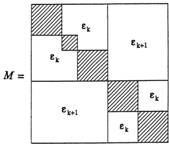
Epsilon decomposition of a square matrix M is concerned with transforming M by symmetric row and column permutations into a form

PTMP = MD + eMC

(49.105)

where MD is block diagonal, and e is a prescribed small number [27]. The problem is equivalent to identifying the connected

components of a subgraph D6 of the digraph D associated with M, which is obtained by deleting all edges of D corresponding to those elements of M with magnitude smaller than 6. All of the vertices of a connected component of D61 appear in the same connected component of D62 for any 62 < e1. Thus one can identify a number of distinct values 61 > 62 > > 6K such that

PTMP = (. . . ((Mo +61M1) + €2M2)

+...+€KMK), (49.106)

which is a nested epsilon decomposition of M as illustrated in Figure 49.3.

7 A

3k

VA, 8k+1

2k

7

8l(+l % 8!:

Figure 49.3 Nested epsilon decompositions.

As seen from theﬁgure, a large 6 results in a ﬁner decomposi-tion than a small 6 does. Thus the choice of 6 provides a compro-mise between the size and the number of components and the strength of the interconnections among them. A nice property of nested epsilon decompositions is that once the decomposition corresponding to some 6k is obtained, the decomposition corre-sponding to 6k+1 can be found by working with a smaller digraph obtained by condensing Dek with respect to its components.

An immediate application of the nested epsilon decomposi-tions is the stability analysis of a large scale system via vector Liapunov functions, where the matrix M is identiﬁed with the matrix A of the system in (6). Provided the subsystems result-ing from the decomposition are stable, the stability of the overall system can easily be established by means of the aggregate matrix W in (49), whose off—diagonal elements are of the order of e.

The nested epsilon decomposition algorithm can also be ap-plied with some modiﬁcations to decompose a system with inputs as

N

56:

=

Aiixi + Biiui +6 Z<Aijxj + Bijuj),

1751'

i e N.

(49.107)

If each decoupled subsystem identiﬁed by a pair (Au, Big) is stabilized by a local state feedback of the form u; = —K,-x,- , i e N, with the local gains not excessively high, then the closed—loop

(13)

49. 8. GRAPH-THEORETIC DECOMPOSITIONS system preserves the weak—coupling property of the Open—loop system, providing an easy way to stabilize the overall system. The same idea can also be employed in designing decentralized estimators [30] based on a suitable epsilon decomposition of the pair (A, C).

49.8.4 Overlapping Decompositions

Consider a system

5: £0) = 21m) (49.108) with an ii—dimensional state vector 55. Let columns of the matrix V E lR'~l X" form a basis for an n—dimensional A-invariant sub-space of R5, and let A be the restriction of A to ImV 2 R", that is, AV = VA. Then the smaller order system

S: 5c(t) = Ax(t) (49.109)

is called a restriction of g. Conversely, starting with the system 8, one can obtain an expansion § of S by deﬁning A = VA VL + M, where VL is any left inverse of V, and M is any complementary matrix satisfying M V = 0. The very deﬁnitiOn of a restriction implies that S is stable if g is.

In many problems associated with large scale systems, it may be desirable to expand a system S to a larger dimensional one which possess some nice structural properties. The increase in dimensionality of the problem may very well be offset by the nice structure of the expansion. As an example, consider a system S with

A11 A12 6A13

A = 6A21 A22 6A23 (49.110)

6 A31

A32

A33

where e is a small parameter. Letting 11 0 0

0 I2 0

V — O [2 0 (49.111)

0 0 [3

where Ik denotes an identity matrix of order nk, one obtains an expansion 8 with

A11 A12 0 6 A13

~ 6A21 A22 0 6A23

= 49.112

A 6A2] 0 A22 €A23 ( )

6 A31 0 A32 A33

Since 5 has an obvious decomposition into two weakly coupled subsystems, one can take advantage of this structural property in stability analysis, which is not available for the original system 8. One can easily notice from the structure of V in (114) that the expansion g of S is obtained simply by repeating the equation for the middle part x2 of the state vector x = [xlT s x3? ] T. In some sense, x2 is treated as common to two overlapping components £1 = [xlT x2T ] T and £2 = [s x; ] T of x. Thus the partitioning of the A matrix in (113) is termed the overlapping decomposition.

791 Although the expansion matrix V can be any matrix with full column rank, if it is restricted to contain one and only one unity element in each row (which corresponds, as in the case above, to repeating some of the state equations in the expanded domain), then one can develop a suitable graph—theoretic algorithm toﬁnd the smallest expansion which has a disjoint decomposition (into decoupled or e—coupled components) with the property that no component is further decomposable.

The idea of overlapping decompOsitions via expansions can be extended to systems with inputs. A system

9 52(1)

=

A560) + Bum

(49.113)

is said to be an expansion of

8: x0) = Ax(t) + Bu(t) (49.114) if E = VB in addition to AV = VA. Consider the optimal control problems of minimizing the performance criteria

I

foo[xT(t)Qx(t) + uT(t)Ru(t)]dt

0

i = /oo[£T(t)Q£(t)+uT(t)Ru(t)]dt (49.115)

0

associated with S and §. The optimal solutions are

u(t) = —Kx(t), and u(t) = 4290),

(49.116)

respectively, resulting in closed—loop systems

s: £0) =

(A — BK)x(t),

§. 5E0) = (ii — 312mm. (49.117) Thus, S is a restriction of§ if (A - 316V = V(A — BK), or equivalently, if I? = K V. The last condition is satisﬁed if Q and Q are related as Q = VT QV, in which case the optimal cost matrices are also related as P = VTISV. This analysis shows that, if the cost matrices Q and R of the expanded system are chosen to be block diagonal with diagonal blocks associated with the decoupled expanded subsystems, then its optimal (in case of complete decoupling) or suboptimal (in case ofweak decoupling) solution can be contracted back to an optimal or suboptimal solution of the original system with respect to a suitably chosen performance criterion.

References

[1] Anderson, B. D. O. and Clements, D. I., Algebraic characterization of ﬁxed modes in decentralized con-trol,Automatica, 17, 703—712, 1981.

[2] Brusin, V. A. and Ugrinovskaya, E. Ya., Decentralized adaptive control with a reference model, Avtomatika i Telemekhanika, 10, 29—36, 1992.

[3] Chae, S. and Bien, 2., Techniques for decentralized control for interconnected systems, in Control and Dynamic Systems, C. T. Leondes, Ed., Academic Press, Boston, 41, 273—315, 1991.

(14)

[4]

[5]

[6]

[7]

[8]

[9]

[10]

[11]

[12]

[13]

[14]

[15]

[16]

[17]

[18]

[19]

[20]

[21]

Chen, Y. H., Decentralized robust control design for large—scale uncertain systems: The uncertainty is time—varying, 1. Franklin Institute, 329, 25—36, 1992. Chen, Y. H. and Han, M. C., Decentralized control de-sign for interconnected uncertain systems, in Control and Dynamic Systems, C. T. Leondes, Ed., Academic Press, Orlando, FL, 56, 219—266, 1993.

Cheng, C. R, Wang, W. 1., and Lin, Y. P., Decentral-ized robust control of decomposed uncertain inter-connected systems, Trans. ASME, 115, 592—599, 1993. Cho, Y. 1. and Bien, Z., Reliable control via an addi-tive redundant controller, Int. 1. Control, 50, 385—398, 1989.

Date, R. A. and Chow, 1. H., A parametrization ap-proach to optimal H2 and H00 decentralized control problems, Automatica, 29, 457—463, 1993.

Datta, A., Performance improvement in decentral-ized adaptive control: A modiﬁed model reference scheme, IEEE Trans. Automatic Control, 38, 1717— 1722, 1993.

Gajié, Z. and Shen, X., Parallel Algorithmsfor Optimal Control ofLarge Scale Linear Systems, Springer—Verlag, Berlin, Germany, 1993.

Geromel, 1. C., Bernussou, 1., and Peres, P. L. D., Decentralized control through parameter space op-timization, Automatica, 30, 1565—1578, 1994. Gﬁndes, A. N. and Kabuli, M. G., Reliable decentral— ized control, Proc. Am. Control Conf., Baltimore, MD,

pp. 3359—3363, 1994.

Iftar, A., Decentralized estimation and control with overlapping input, state, and output decomposition, Automatica, 29, 511-516, 1993.

Ikeda, M., Decentralized Control of Large Scale Systems, in Three Decades of Mathematical System Theory, H. Nijmeiyer and 1. M. Schumacher, Eds., Springer-Verlag, New York, 1989, 219—242.

1amshidi, M., Large—Scale Systems. Modeling and Con-trol, North—Holland, New York, 1983.

Lakshmikantham, V. and Liu, X. Z., Stability Analysis In Terms ofTwo Measures, World Scientiﬁc, Singapore, 1993.

Lakshmikantham, V., Matrosov, V. M., and Sivasun-daram, 8., Vector Liapunov Functions and Stability Analysis of Nonlinear Systems, Kluwer, The Nether-lands, 1991.

Leitmann, G., One approach to the control of uncer-tain systems, ASME I. Dyn. Syst., Meas., and Control,

115, 373—380, 1993.

Leondes, C. T., Ed., Control and Dynamic Systems, Vols. 22-24, Decentralized/Distributed Control and Dynamic Systems, Academic Press, Orlando, FL, 1985.

Lin, C. T., Structural controllability, IEEE Trans. Auto. Control, AC—19, 201—208, 1974.

Lyon, 1., Note on decentralized adaptive controller design, IEEE Trans. Auto. Control, 40, 89—91, 1995.

[22] Michel, A. N., On the status of stability of intercon-nected systems, IEEE Trans. Circuits Syst., GAS—30, 326—340, 1983.

[23] Mills, 1. K., Stability of robotic manipulators during transition to and from compliant motion, Automat-ica, 26, 861—874, 1990.

[24] Sandell, N. R., 1r., Varaiya, P., Athans, M., and Sa-fonov, M. G., Survey of decentralized control meth-ods for large scale systems, IEEE Trans. Auto. Control, AC—23, 108—128, 1978.

[25] Savastuk, S. V. and Siljak, D. D., Optimal decentral-ized control, Proc. Am. Control Conf., Baltimore, MD,

pp. 3369—3373, 1994.

[26] Sezer, ME. and Siljak, D. D., Structurallyﬁxed modes, Syst. Control Lett, 1, 60—64, 1981.

[27] Sezer, M. E. and Siljak, D. D., Nested 6-decomposition and clustering of complex systems, Automatica, 22, 321—331, 1986.

[28] Shi, L. and Singh, S. K., Decentralized adaptive con-troller design for large—scale systems with higher or-der interconnections, IEEE Trans. Auto. Control, 37, 1106—1118,1992.

[29] Siljak, D. D., Large—Scale Dynamic Systems: Stability and Structure, North—Holland, New York, 1978. [30] Siljak, D. D., Decentralized Control of Complex

Sys-tems, Academic Press, Cambridge, MA, 1991. [31] Tamura, H. and Yoshikawa, T., Large—Scale Systems

Control and Decision Making, Marcel Dekker, New York, 1990.

[32] Unyelioglu, K. A. and Ozgiiler, A. B., Reliable decen-tralized stabilization offeed—forward and feedback in-terconnected systems, IEEE Trans. Auto. Control, 37,

1119—1132, 1992.

[33] Voronov, A. A., Present state and problems ofstability theory, Automatika i Telemekhanika, 5, 5—28, 1982. [34] Wang, S. H. and Davison, E. 1., On the stabilization

of decentralized control systems, IEEE Trans. Auto. Control, AC—l8, 473:478, 1973.

[35] Wu, W. and Lin, C., Optimal reliable control system design for steam generators in pressurized water re-actors, Nuclear Technology, 106, 216—224, 1994. [36] Yu, R., Ocali, O., and Sezer, M. E., Adaptive

ro-bust sampled—data control of a class of systems under structured perturbations, IEEE Trans. Auto. Control, 38, 1707—1713, 1993.

[71,[12Ll32],

[35]-In a recent development [25], it has been shown how opti-mal decentralized control oflarge scale interconnected sys-tems can be obtained in the classical optimization frame-work of Lagrange. Both sufﬁcient and necessary conditions for optimality are derived in the context of Hamilton-Jacobi equations and Pontryagin’s maximum principle.