Full Terms & Conditions of access and use can be found at
http://www.tandfonline.com/action/journalInformation?journalCode=uaai20
An International Journal
ISSN: 0883-9514 (Print) 1087-6545 (Online) Journal homepage: http://www.tandfonline.com/loi/uaai20
Human Activity Recognition Using Tag-Based Radio
Frequency Localization
Aras Yurtman & Billur Barshan
To cite this article: Aras Yurtman & Billur Barshan (2016) Human Activity Recognition Using Tag-Based Radio Frequency Localization, Applied Artificial Intelligence, 30:2, 153-179, DOI: 10.1080/08839514.2016.1138787
To link to this article: https://doi.org/10.1080/08839514.2016.1138787
Published online: 15 Mar 2016.
Submit your article to this journal
Article views: 106
View related articles
View Crossmark data
Human Activity Recognition Using Tag-Based Radio
Frequency Localization
Aras Yurtman and Billur Barshan
Department of Electrical and Electronics Engineering, Bilkent University, Bilkent, Ankara, Turkey
ABSTRACT
This article provides a comparative study on the different techniques of classifying human activities using tag-based radio-frequency (RF) localization. A publicly available dataset is used where the position data of multiple RF tags worn on different parts of the human body are acquired asynchronously and nonuniformly. In this study, curves fitted to the data are resampled uniformly and then segmented. We investigate the effect on system accuracy of varying the relevant system para-meters. We compare various curve-fitting, segmentation, and classification techniques and present the combination result-ing in the best performance. The classifiers are validated usresult-ing 5-fold and subject-based leave-one-out cross validation, and for the complete classification problem with 11 classes, the proposed system demonstrates an average classification error of 8.67% and 21.30%, respectively. When the number of classes is reduced to five by omitting the transition classes, these errors become 1.12% and 6.52%, respectively. The results indi-cate that the system demonstrates acceptable classification performance despite that tag-based RF localization does not provide very accurate position measurements.
Introduction and related work
With rapidly developing technology, devices such as personal digital assis-tants (PDAs), tablets, smartphones, and smartwatches have made their way into our daily lives. It is now becoming essential for such devices to recognize and interpret human behavior correctly in real time. One aspect of these context-aware systems is recognizing and monitoring daily activities such as sitting, standing, lying down, walking, ascending/descending stairs, and most
importantly, falling (Özdemir and Barshan2014).
Several different approaches for recognizing human activities exist in the
literature (Logan et al. 2007; Yurtman and Barshan 2014). A large number of
studies employ vision-based systems with multiple video cameras fixed to the environment in order to recognize a person’s activities (Marín-Jiménez, Pérez de CONTACTBillur Barshan [email protected] Department of Electrical and Electronics Engineering, Bilkent University, Bilkent, TR-06800 Ankara, Turkey.
Color versions of one or more of the figures in the article can be found online atwww.tandfonline.com/UAAI. 2016, VOL. 30, NO. 2, 153–179
http://dx.doi.org/10.1080/08839514.2016.1138787
la Blanca, and Mendoza2014; Moeslund, Hilton, and Krüger2006; Wang, Hu,
and Tan 2003; Aggarwal and Cai, 1999). In many of these studies, points of
interest on the human body are pre-identified by placing visible markers such as light-emitting diodes (LEDs) on them and recording the positions with cameras
(Sukthankar and Sycara2005). For example, the study reported in (Luštrek and
Kaluža2009) considered a total of six activities, including falls, using an infrared
motion capture system. As attributes, they used body part positions in different coordinate systems and angles between adjacent body parts. In Luštrek et al.
(2009), walking anomalies such as limping, dizziness, and hemiplegia were
detected using the same system. Camera systems obviously interfere with priv-acy because they capture additional information that is not needed by the system but that might easily be exploited with a simple modification to the software. Further, people usually act unnaturally and feel uncomfortable when camera systems are used, especially in private places. Other disadvantages of vision-based systems are the high computational cost of processing images and videos; correspondence and shadowing problems; the need for camera calibration; and inoperability in the dark. When multiple cameras are employed, several 2D projections of the 3D scene must be combined. Moreover, this approach imposes restrictions on the person’s mobility because the system operates only in the limited environment monitored by the cameras.
A second approach utilizes wearable motion sensors, whose size, weight, and cost have decreased considerably in the last two decades (Altun, Barshan, and
Tunçel 2010; Barshan and Yüksek 2014; Barshan and Yurtman 2016). The
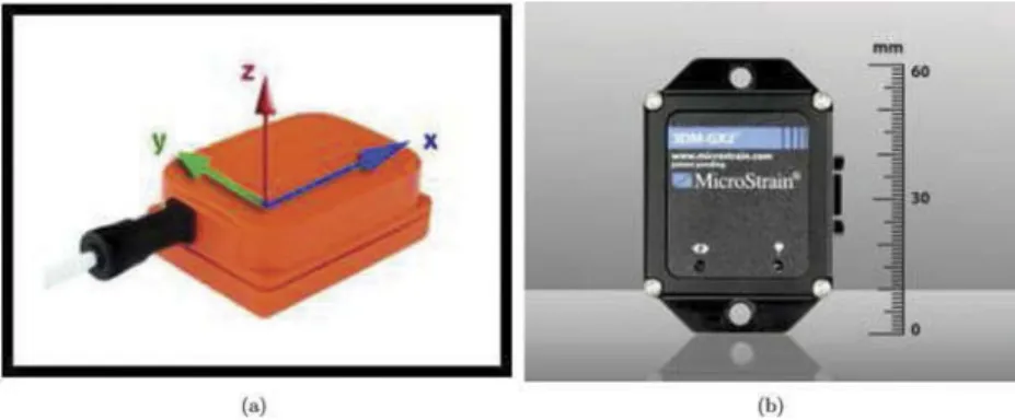
availability of such lower-cost and medium-performance units has opened new possibilities for their use. In this approach, several motion sensor units are worn on different parts of the body. These units usually contain gyroscopes and accelerometers, which are inertial sensors, and sometimes also magnet-ometers. Some of these devices are sensitive around a single axis, whereas others
are multiaxial (usually two- or three-axial). Two examples are shown inFigure 1,
and a wearable system is illustrated inFigure 2(a).
Inertial sensors do not directly provide linear or angular position informa-tion. Gyroscopes provide angular rate information around an axis of sensi-tivity, whereas accelerometers provide linear or angular velocity rate information. These rate outputs need to be integrated once or twice to obtain the linear/angular position. Thus, even very small errors in the rate informa-tion provided by inertial sensors cause an unbounded growth in the error of integrated measurements.
The acquired measurements are either collected and processed in a battery-powered system such as a cellular phone, or wirelessly transmitted to a com-puter for processing. Detailed surveys on activity recognition using inertial
sensors can be found in the literature (Altun, Barshan, and Tunçel 2010;
Sabatini 2006; Zijlstra and Aminian 2007; Mathie et al. 2004; Wong, Wong,
Figure 2.(a) Motion sensor units worn on the body (Xsens 2016) © Xsens. Reproduced by permission of Xsens. Permission to reuse must be obtained from the rightsholder. (b) An active RFID tag (SYRIS SYSTAG245-TM-B) worn as a bracelet (SYRIS 2016) © SYRIS. Reproduced by permission of SYRIS. Permission to reuse must be obtained from the rightsholder. (c) An RFID tag inserted under the skin © GeekWire.com. Reproduced by permission of GeekWire.com. Permission to reuse must be obtained from the rightsholder. (d) Tiny RFID tags of size 2mm x 2mm © Tagent Corp. Reproduced by permission of Tagent Corp. Permission to reuse must be obtained from the rightsholder.
and Lo2007). We used inertial sensors in our earlier work on human activity
recognition (Altun, Barshan, and Tunçel 2010; Altun and Barshan 2010;
Ayrulu-Erdem and Barshan 2011; Tunçel, Altun, and Barshan 2009), and
although this method results in accurate classification, wearing the sensors and the processing unit on the body might not always be comfortable or even acceptable, despite how small and lightweight they have become. Further, people might forget or neglect to wear these devices. This approach has other limitations: Although we have demonstrated that it is possible to recognize activities with high accuracy (typically above 95%), the same is not true for human localization because of the drift problem associated with inertial sensors
(Altun and Barshan 2012; Welch and Foxlin 2002). In Altun and Barshan
(2012), we exploited activity cues to improve the erroneous position estimates
provided by inertial sensors and achieved significantly better accuracies when localization was performed simultaneously with activity recognition. Ogris et al.
(2012) describe the design and evaluation of pattern analysis methods for the
recognition of maintenance-related activities (hands tracking) using a combi-nation of inertial and ultrasonic sensors.
Rather than monitoring human activities from a distance or remotely, we
believe that“activity can best be measured where it occurs,” as stated in Kern,
Schiele, and Schmidt (2003). Unlike computer vision systems, the second
approach described previously directly acquires motion data, and the third approach (which we use in this study) directly acquires position data in 3D.
The latter uses the radio-frequency (RF) localization technique1to record the
3D positions of RF tags worn on different parts of the body. The size and cost of these sensors are comparable to inertial sensors but they require an instrumented environment, whereas this is not needed for inertial sensors. In an RF localization system, there are multiple antennas, called readers, mounted in the environment that detect the relative positions of small
devices called RF tags (Figure 2(b)–(d)). Each tag emits RF pulses containing
its unique ID for identification and localization. Active RF tags have internal power sources (batteries) to transmit RF pulses, whereas passive tags do not contain a power source and rely on the energy of the waves transmitted by
the readers (Zhang, Amin, and Kaushik 2007). Passive RF tags are stickers
similar to radio-frequency identification (RFID) tags, and can be as small as
2 mm × 2 mm (Figure 2(d)), whereas active RF tags are much larger
(Figure 2(b)). RF tags are inexpensive and lightweight and thus comfortable
for use on the human body (Weis2012). Unlike bar codes, the tag does not
1
Radio-Frequency Identification (RFID) involves tag detection and identification (deciding which tags exist in the environment), whereas in RF localization, tags are identified and localized. The tags are called“RFID tags” in the former system and“RF tags” in the latter, although they can be identical in some cases (Bouet and dos Santos 2008; Zhang, Amin, and Kaushik2007). In this text, the tags used for localization are not the same as RFID tags, hence, they will be called“RF tags.” In some texts, the term “RFID localization” is used instead of “RF localization” because there are systems estimating the positions of RFID tags that are designed for identification only (Bouet and dos Santos2008).
need to be in the reader’s line of sight; it can be embedded in the tracked
object or even inserted under the skin (Figure 2(c)).
The operating range of most RF readers is not more than 10 m (Liu et al.
2007). In uncluttered, open environments, typical localization accuracy is about
15 cm across 95% of the readings (Steggles and Gschwind2005). Because each
tag must be detected by multiple readers for localization, this method cannot be used in large areas because numerous readers would be needed, and that would be too costly. Further, the number of RF tags that can be worn on the body is limited. In systems that use active tags, the pulses transmitted by the tags may interfere with each other, whereas with passive tags, it is difficult for the system to distinguish between tags that are close together.
RFID technology is a valuable tool in a variety of applications involving automatic detection, identification, localization, and tracking of people,
ani-mals, vehicles, baggage, and goods (Want 2006). An excellent review of the
academic literature on this topic can be found in Ngai et al. (2008). RFID
systems are used for general transport logistics, collecting tolls and contactless payment, tracking parcels and baggage, and deterring theft from stores. With RFID tags, assembly lines and inventories in the supply chain can be tracked more efficiently and products become more difficult to falsify. This attribute is particularly important for the pharmaceutical industry, with its increasing need
for anticounterfeit measures (Yue, Wu, and Bai2008). RFID tags are also used
for identifying and tracking pets, farm animals, and rare animal species such as pandas. They are in contactless identity cards for managing access to and monitoring of hospitals, libraries, museums, schools and universities, and restricted zones. Machine readable identification and travel documents such as biometric passports that contain RFID tags are becoming very common. RFID tags are used for key identification in vehicles, for locking/unlocking vehicles from a distance, ticketing for mass events and public transport, and transponder timing of sporting events.
RFID systems are also suitable for indoor localization and mapping (Ni
et al. 2004). Hahnel et al. (2004) analyze whether RFID technology in the
field of robotics can improve the localization of mobile robots and people in their environment and determine computational requirements. In Choi, Lee,
and Lee (2008), multiple RFID tags are placed on a floor in a grid
config-uration at known positions, and a robot localizes itself by detecting the tags with its antenna. To resolve issues concerning the security and privacy of
RFID systems, Feldhofer, Dominikus, and Wolkerstorfer (2004) propose an
authentication protocol based on RFID tags.
In earlier work on human activity recognition using RFID technology, daily activities are mostly inferred based on a person’s interactions with objects in his/her environment. RFID antennas are usually worn in the form of gloves or bracelets, and RFID tags are fixed to objects in the environment such as equipment, tools, furniture, and doors. The main
limitation of these systems is that they provide activity information only when the subject interacts with one of the tagged objects, thus, the only recognizable activities are those that involve these objects. This type of
approach is followed in several studies (Philipose et al. 2004; Smith et al.
2005; Huang et al. 2010; Wang et al. 2009; Tapia, Intille, and Larson 2004).
Similarly, in (Buettner et al.2009), the authors employ RFID sensor networks
based on wireless identification and sensing platforms (WISPs), which com-bine passive UHF RFID technology with traditional sensors. Everyday objects are tagged with WISPs to detect when they are used, and a simple hidden Markov model (HMM) is used to convert object traces into high-level daily activities such as shopping, doing office work, and commuting. Wu et al.
(2007) present a dynamic Bayesian network model that combines RFID and
video data to jointly infer the most likely household activity and object labels.
Stikic et al. (2008) combine data from RFID tag readers and accelerometers
to recognize ten housekeeping activities with higher accuracy. A multiagent system for fall and disability detection of the elderly living alone is presented
in Kaluža et al. (2010), based on the commercially available Ubisense smart
space platform (Steggles and Gschwind 2005).
A necessary aspect of most RF systems is that the system measures the tag positions asynchronously and nonuniformly at different, arbitrary time instants. In other words, whenever the readers receive a pulse transmitted by an RF tag, the system records its relative position along the x, y, and z axes as well as a unique timestamp and its unique ID. Although each tag transmits pulses periodically, tags cannot be synchronized because their pulses must not interfere with each other; thus, tag locations are sampled at different time instants. Furthermore, readers sometimes cannot detect pulses due to low signal-to-noise ratio (SNR), interference, or occlusion. Under these circumstances, localization accuracy might drop significantly. The detection ratio of a tag increases when it is close to the antennas and decreases when it is near conductive objects such as a metal surface or a computer. Thus, it is not possible to treat the raw measurements as ordinary position vectors sampled at a constant rate in time. In
Hapfelmeier and Ulm (2014), variable selection has been suggested for
random forests to improve data prediction and interpretation when data with missing values are used.
In this study, we consider a broad set of daily activity types (11 activities) and recognize them with high accuracy without having to account for a person’s interaction with objects in his/her environment. We track the position data of four RF tags worn on the body, acquired by the Ubisense
platform (Steggles and Gschwind 2005) and provided as a publicly available
dataset. In the data preprocessing stage, we propose a method to put the dataset in a uniform and synchronously sampled form. After feature reduc-tion in two different ways, we compare several classifiers through P-fold and
subject-based leave-one-out (L1O) cross-validation techniques. We investi-gate variations of the relevant system parameters on the classification performance.
This article is organized as follows. In“The System Details,” we provide details
of the experimental setup and the dataset. Following that, we describe
preproces-sing of the dataset.“Feature Extraction and Reduction” is explored, followed by
listing the classifiers for activity recognition in“Classification.” In “Performance
Evaluation Through Cross Validation,” we evaluate the classifier performance
through the use of two cross-validation techniques. In“Experimental Results,” we
present and interpret the experimental results, and in the final section, we draw conclusions and set out possible directions for future research.
The system details
We employed a publicly available dataset in this study (University of California,
Irvine, Machine Learning Repository 2010). The human activity recognition
system from which the dataset was acquired employs four active RF tags worn on different parts of the body, whose relative positions along the three axes are detected by a computer or a simple microcontroller via four RF antennas mounted in the environment. The RF tags are positioned on the left ankle (tag
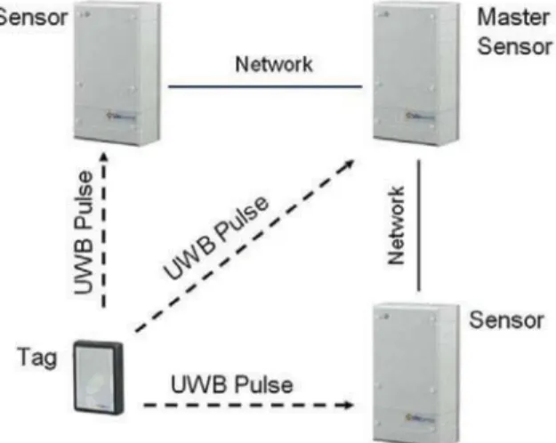
1), right ankle (tag 2), chest (tag 3), and belt (tag 4). In Figure 3, a similar
configuration is shown with three antennas and a single tag.
The 3D position data of a subject’s RF tags are measured over time while she/he performs a fixed sequence of predetermined activities. The operating range of the system is about 46 m. Although each tag transmits a pulse every 0.1 s, the readers might miss some of the pulses (due to occlusion, low SNR at large distances, etc.)
Figure 3.Ubisense hardware components (Steggles and Gschwind 2005). © Ubisense. Reproduced by permission of Ubisense. Permission to reuse must be obtained from the rightsholder.
and therefore, the data acquisition rate is not constant. However, the average detection rate does not much vary and the average sampling rate is 7.2 Hz for the whole dataset.
The 11 activity types are numbered as follows: (1) walking, (2) falling, (3) the process of lying down, (4) lying down, (5) sitting down, (6) sitting on a chair, (7) standing up from lying down, (8) on all fours, (9) sitting on the ground, (10) standing up from sitting on a chair, (11) standing up from sitting on the ground.
Each subject performs a sequence of activities, referred to as an
“experi-ment” in this work. Each experiment consists of the following sequence of activities with different but similar durations:
walking—sitting down—sitting on a chair—standing up from sitting on a chair— walking—falling—lying down—standing up from lying down—walking—the process of lying down—lying down—standing up from lying down—walking—falling—lying down—standing up from lying down—walking—sitting down—sitting on a chair— sitting on the ground—standing up from sitting on the ground—walking—the process of lying down—lying down—standing up from lying down—walking—the process of lying down—on all fours—lying down—standing up from lying down—walking. There are five subjects, each performing the same experiment five times. Thus, there is a total of 5 × 5 = 25 experiments of the same scenario. The
dataset described and used in this study is titled “Localization Data for
Person Activity Data Set” and is publicly available at the University of
California, Irvine, Machine Learning Repository (2010). The dataset is an
extremely long but simple-structured 2D array of size 164,860 × 8 (see
Figure 4 for sample rows). Each line of the raw data corresponds to one measurement, in which the first element denotes the subject code (A–E) and the experiment number (01–05); the second element is the tag ID (the unique ID of one of the four tags); the third column is a unique timestamp; the fourth column is the explicit date and time; the fifth, sixth, and seventh
...
A01, 020-000-032-221, 633790227929538017, 27.05.2009 14:06:32:953, 2.1674482822418213, 1.7744109630584717, 0.768406093120575, standing up from lying down A01, 010-000-024-033, 633790227929808316, 27.05.2009 14:06:32:980, 2.083272695541382, 1.605885624885559, -0.019668469205498695, standing up from lying down A01, 020-000-033-111, 633790227930348903, 27.05.2009 14:06:33:033, 2.1095681190490723, 1.670161485671997, 1.096860647201538, standing up from lying down A01, 020-000-032-221, 633790227930619202, 27.05.2009 14:06:33:063, 2.1871273517608643, 1.8179994821548462, 0.7751449942588806, standing up from lying down A01, 010-000-024-033, 633790227930889495, 27.05.2009 14:06:33:090, 2.124642848968506, 1.3958414793014526, 0.05755209922790527, standing up from lying down A01, 010-000-030-096, 633790227931159787, 27.05.2009 14:06:33:117, 2.3755478858947754, 1.9687641859054565, -0.02469586208462715, walking A01, 020-000-033-111, 633790227931430084, 27.05.2009 14:06:33:143, 2.162515878677368, 1.688720703125, 1.1396502256393433, walking A01, 020-000-032-221, 633790227931700376, 27.05.2009 14:06:33:170, 2.1584346294403076, 1.7068990468978882, 0.7499973177909851, walking A01, 010-000-024-033, 633790227931970674, 27.05.2009 14:06:33:197, 2.007559299468994, 1.7204831838607788, -0.04071690887212753, walking A01, 020-000-032-221, 633790227932781551, 27.05.2009 14:06:33:277, 2.1662490367889404, 1.5868778228759766, 0.9013731479644775, walking ... A01, 020-000-033-111, 633790227969271197, 27.05.2009 14:06:36:927, 3.2222139835357666, 1.994187593460083, 1.0909717082977295, walking A01, 020-000-032-221, 633790227969541489, 27.05.2009 14:06:36:953, 3.3250277042388916, 2.288264036178589, 1.0457459688186646, walking A01, 010-000-024-033, 633790227969811780, 27.05.2009 14:06:36:980, 3.237037420272827, 2.085507392883301, 0.31236138939857483, walking A01, 010-000-030-096, 633790227970082071, 27.05.2009 14:06:37:007, 2.991684675216675, 1.9473466873168945, -0.052446186542510986, walking A01, 020-000-033-111, 633790227970352368, 27.05.2009 14:06:37:037, 3.2356183528900146, 2.0799317359924316, 1.1940621137619019, walking A02, 010-000-024-033, 633790230241677177, 27.05.2009 14:10:24:167, 3.8436150550842285, 2.038317918777466, 0.4496184289455414, walking A02, 010-000-030-096, 633790230241947475, 27.05.2009 14:10:24:193, 3.288137435913086, 1.7760037183761597, 0.2172906994819641, walking A02, 020-000-033-111, 633790230242217774, 27.05.2009 14:10:24:223, 3.7905502319335938, 2.10894513130188, 1.2178658246994019, walking A02, 020-000-032-221, 633790230242488064, 27.05.2009 14:10:24:250, 4.826080322265625, 3.061596393585205, 2.016235589981079, walking A02, 010-000-024-033, 633790230242758363, 27.05.2009 14:10:24:277, 3.889177083969116, 1.9832324981689453, 0.34168723225593567, walking A02, 010-000-024-033, 633790230243839526, 27.05.2009 14:10:24:383, 3.8668057918548584, 2.037929058074951, 0.4540541470050812, walking A02, 010-000-030-096, 633790230244109820, 27.05.2009 14:10:24:410, 3.724804401397705, 2.37532639503479, 0.43077021837234497, walking A02, 020-000-033-111, 633790230244380118, 27.05.2009 14:10:24:437, 3.798861265182495, 2.0785067081451416, 1.1724120378494263, walking A02, 020-000-032-221, 633790230244650412, 27.05.2009 14:10:24:467, 4.824059009552002, 3.062581777572632, 2.010768413543701, walking A02, 010-000-024-033, 633790230244920703, 27.05.2009 14:10:24:493, 3.889165163040161, 2.053361177444458, 0.3612026274204254, walking A02, 020-000-033-111, 633790230245461287, 27.05.2009 14:10:24:547, 3.8123855590820312, 1.9204648733139038, 1.1589833498001099, walking ...
columns, respectively, contain the relative x, y, and z positions of the tag; and the eighth column stores the event name, corresponding to one of the 11 activities performed. We modified the dataset such that each activity type is represented by its number for simplicity without loss of information. Similarly, the unique IDs of the tags in the raw data are converted to tag numbers 1–4 for the sake of simplicity and without loss of information. Note that a measurement corresponding to one row of the dataset simply defines the relative position of a particular tag at a particular time instant (as well as the true activity type) and is acquired by multiple antennas. The data for each experiment are just a subset of the rows in the raw data array. Therefore, the sequence of activities and their durations can be extracted
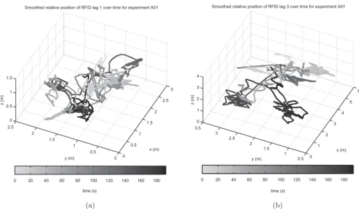
from the dataset. As an example, inFigure 5we show the positions of tags 1
and 3 in the first experiment of the first subject as 3D curves in time, with the gray level of the curve changing from light gray to black as time passes. An important problem in activity recognition is detecting activity durations and transition times in a continuous data stream (Junker
et al. 2008; Guenterberg et al. 2009; Bicocchi, Mamei, and Zambonelli
2010; Mannini and Sabatini 2010). In the dataset, activities 2, 3, 5, 7, 10,
and 11 actually correspond to transitions between two activities, and their duration is much shorter than the others. For example, class 5 (sitting down) stands for the change from the state of walking to the state of sitting on a chair. In the original dataset, these transition activities are assigned to ordinary activity classes so that there is a total of 11 activities. In addition to the classification problem with 11 classes, we consider a
0 0.5 1 1.5 2 2.5 3 0 0.5 1 1.5 2 2.5 0 0.5 1 1.5 x (m) Smoothed relative position of RFID tag 1 over time for experiment A01
y (m) z (m) 0 20 40 60 80 100 120 140 160 180 time (s) (a) 0 1 2 3 4 5 6 0.5 1 1.5 2 2.5 3 3.5 0 1 2 3 4 x (m) Smoothed relative position of RFID tag 3 over time for experiment A01
y (m)
z (m)
0 20 40 60 80 100 120 140 160 180 time (s)
(b)
Figure 5.The positions of (a) tag 1 and (b) tag 3 in the first experiment of the first subject as 3D curves whose gray level changes from light gray to black over time.
simplified (reduced) case with five classes (corresponding to activities 1, 4, 6, 8, and 9) by omitting the transition classes.
Preprocessing of the data
Curve fitting
Because tag positions are acquired asynchronously and nonuniformly, feature extraction and classification based on the raw data would be very difficult. Thus, we first propose to fit a curve to the position data of each axis of each tag (a total of 3 × 4 = 12 axes) in each experiment and then resample the fitted curves uniformly at exactly the same time instant. Provided that the new, constant sampling rate is considerably higher than the average data acquisition rate, the curve-fitting and resampling process does not cause much loss of information. We assume that the sample values on the fitted curves (especially those that are far from the actual measurement points) represent the true positions of the tags because the tag positions do not change very rapidly. In general, tag positions on arms and legs tend to change faster than on chest and waist.
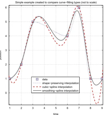
Three curve-fitting methods are considered in this work:
(1) In shape-preserving interpolation, the fitted curve passes through the measurement points, around which it is curvy and smooth but in between looks almost like straight lines. Hence, this method is very similar to linear (or first-order) interpolation, except that the curve is differentiable everywhere. The fitted curve has a high curvature, espe-cially around the peaks.
(2) The second method is cubic-spline interpolation. The curve in this method also passes through the measurement points but overall is much smoother. The fitted curve might oscillate unnecessarily between the measurement points and may go far beyond the peaks of the measurements, in which case, it might not resemble (one axis of) the actual position curve of the tag.
(3) The smoothing spline is the third method, having a single parameter adjustable between 0 and 1. It is observed that this method resembles a shape-preserving interpolant when the parameter is chosen to be about 0.5 and resembles a cubic-spline interpolant when it is approxi-mately 1. The parameter value should be chosen to be proportionately large with the complexity of the data, i.e., the number of available position measurements. In this study, we used a parameter value of
Although the third method seems to provide better results than the others, it is not feasible for long data (as in this study) because its computational complexity is much higher. Therefore, for its simplicity, we preferred to use the shape-preserving interpolation. Sample curves fitted to synthetic position
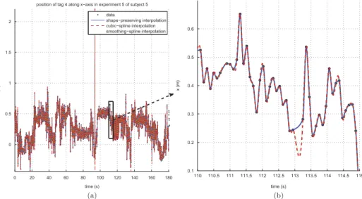
data using the three methods are plotted in Figure 6. In addition, in Figure 7,
we plot the x position of tag 4 in the fifth experiment of the fifth subject. Once the 12 different curves are fitted to the 12 axes of each experiment indepen-dently, the curves are resampled uniformly at exactly the same time instants.
Segmentation
After the curve fitting and uniform resampling stages, the modified dataset now consists of 5 × 5 = 25 2D arrays (each corresponding to an experiment), with each line containing the time instant, position values along the 12 axes (three axes per tag) at that instant, and the activity being performed at that time. Note that the number of rows is not the same for all experiments because the duration of the experiment and, hence, the number of equally spaced samples, might differ slightly.
The 2D array of each experiment is first divided into intervals containing samples corresponding to exactly one activity type. Then, each interval is divided into time segments of equal length, typically about one second. To
1 2 3 4 5 6 7 8 9 0 1 2 3 4 5 6 time position
Simple example created to compare curve−fitting types (not to scale)
data
shape−preserving interpolation cubic−spline interpolation smoothing−spline interpolation
prevent a segment from containing more than one activity, the following segmentation rule is used: For each experiment, progressing vertically along the 2D array, a new segment is started only if the desired segment length is reached or a different activity is encountered. Naturally, the segments imme-diately before the transition points between activities and the very last segment may be shorter in length.
We classify each segment independently. When testing the classifiers and implementing the system in real time, the system needs to know where a new activity starts (i.e., the activity transition times). Since various techniques for modeling activity durations and detecting activity transition times are available
(Junker et al. 2008; Duong et al. 2005), we performed segmentation based on
the information on the true transition times so that each segment is associated with only a single activity. If it is not possible to use a constant segment duration throughout, some of the segments may be associated with more than one activity. One can assign the longest activity contained in that segment as the true class, but this would unfairly decrease the classification accuracy.
Feature extraction and reduction
Feature extraction
As stated, each segment consists of many position samples in the correspond-ing time interval: Each row of the dataset comprises 13 values (one time instant and 12 position values) and the true activity class. Thus, it would take a lot of time for a classifier to be trained and evaluated using the whole
0 20 40 60 80 100 120 140 160 180 0 0.5 1 1.5 2 time (s) x (m)
position of tag 4 along x−axis in experiment 5 of subject 5 data shape−preserving interpolation cubic−spline interpolation smoothing−spline interpolation (a) 110 110.5 111 111.5 112 112.5 113 113.5 114 114.5 115 0.1 0.2 0.3 0.4 0.5 0.6 time (s) x (m) (b)
Figure 7.Thex position of tag 4 in the fifth experiment of the fifth subject. (a) The whole curve and (b) the zoomed-in version.
data. As an alternative, we use features extracted from the time segments for classification.
The features extracted for each of the 12 axes are the minimum, maximum, mean, variance, skewness, and kurtosis values, the first few coefficients of the autocorrelation sequence, and the magnitudes of five or fewer Fast Fourier
Transform (FFT) peaks2. Therefore, there are (12 axes × [11 + ceil(N/2)]
coefficients per axis) = 132 + 12 × ceil(N/2) coefficients in the feature vector, N being the maximum number of samples in a segment (N = 5 in this study). Note that the size of the feature vector increases with the maximum number of samples in a segment, which, in turn, is the product of the sampling frequency (in Hz) and the segment duration (in s).
Feature reduction
Because of the large number of features (about 150–200) associated with each segment, we expect feature reduction to be very useful in this scheme. The size of the feature vector is reduced by mapping the original high-dimensional feature space to a lower-dimensional one using principal component analysis
(PCA) (Alfaro et al.2014) and linear discriminant analysis (LDA) (Duda, Hart,
and Stork 2001). PCA is a transformation that finds the optimal linear
combination of the features, representing the data with the highest variance in a feature subspace without separately considering intraclass and interclass variances. It seeks a projection that best represents the data in a least-squares sense. On the other hand, LDA seeks a projection that best separates the data in the same sense and maximizes class separability (Duda, Hart, and Stork
2001). Whereas PCA seeks rotational transformations that are efficient for
representation, LDA seeks those that are efficient for discrimination. The best projection in LDA makes the difference between the class means as large as possible relative to the variance.
Classification
Following are the ten classifiers used in this study, with their corresponding
PRTools (Duin et al.2007) functions:
(1) ldc: Gaussian classifier with the same arbitrary covariance matrix for each class
(2) qdc: Gaussian classifier with different arbitrary covariance matrices for each class
2If there are fewer than five time samples in a given segment, the number of FFT peaks is as many as the number
(3) udc: Gaussian classifier with different diagonal covariance matrices for each class
(4) mogc: mixture of Gaussian classifiers (with two mixtures) (5) naivebc: naïve Bayes classifier
(6) knnc: k-nearest neighbor (k-NN) classifier (7) kernelc: dissimilarity-based classifier
(8) fisherc: minimum least-squares linear classifier (9) nmc: nearest mean classifier
(10) nmsc: scaled nearest mean classifier
Detailed descriptions of these classifiers can be found in (Duda, Hart, and
Stork 2001).
Performance evaluation through cross validation
Because each of the five subjects repeats the same sequence of activities five times, the procedures used for training and testing affect the classification accuracy. For this reason, we use two cross-validation techniques for evalu-ating the classifiers: P-fold and subject-based L1O (Duda, Hart, and Stork
2001).
In P-fold cross validation (P = 5 in this article), the whole set of feature vectors is divided into P partitions, where the feature vectors in each partition are selected randomly, regardless of the subject or the class they belong to. One of the P partitions is retained as the validation set
for testing, and the remaining P − 1 partitions are used for training. The
cross-validation process is then repeated P times (the folds), so that each of the P partitions is used exactly once for validation. The P results from the folds are then averaged to produce a single estimate of the overall classification accuracy.
In subject-based L1O cross validation, partitioning of the dataset is done subject-wise instead of randomly. The feature vectors of four of the subjects are used for training and the feature vectors of the remaining subject are used for validation. This is repeated five times such that the feature vector set of each subject is used once as the validation data. The five correct classification rates are averaged to produce a single estimate. This is same as P-fold cross validation with P being equal to the number of subjects (P = 5) and all the feature vectors in the same partition being associated with the same subject. We have selected P to be the same as the number of subjects in P-fold cross validation to use the same number of training vectors in the two cross-validation techniques; hence, to allow a fair comparison between them.
Although these two cross-validation methods use all the data equally in training and testing the classifiers, there are two factors that affect the results
obtained based on the same data. The first is the random partitioning of the data in the P-fold cross-validation technique, which slightly affects the classi-fication accuracy. Second, classifier 7 (the dissimilarity-based classifier) includes randomness in its nature. Therefore, both cross-validation methods are repeated five times and the average classification accuracy and its standard deviation are calculated over the five executions. In this way, we can assess the repeatability of the results and estimate how well the system will perform over newly acquired data from unfamiliar subjects.
Experimental results
The following are the adjustable parameters or factors that might affect classification accuracy, with their default values written in square brackets:
(1) fs: sampling frequency of the fitted curves in forming the modified data (in Hz) [default: 10 Hz]
(2) frm_dur: maximum segment duration (in seconds) [default: 0.5 s] (3) curve_fit_type: the curve-fitting algorithm
(1: shape-preserving interpolation, 2: cubic-spline interpolation, 3: smoothing-spline interpolation) [default: 1]
(4) pri: prior probabilities of the 11 classes (i.e., activities)
(0: equal priors for each class, 1: priors calculated based on class frequencies) [default: 1]
(5) reduc: the feature reduction type if used and the dimension of the
reduced feature space (0: no feature reduction; + nj j: PCA with reduced
dimension n; − nj j: LDA with reduced dimension n) [default: 0]
All classifiers are trained and tested using different combinations of the parameters described above by sampling the parameter space uniformly. Then, for each classifier, the set of parameters that results in the lowest average classification error is determined. This process is repeated for both cases (the complete and simplified classification problems with 11 and 5 classes, respec-tively) and both cross-validation methods (5-fold and subject-based L1O). Average classification errors of the classifiers over the five executions and their
standard deviations are given inTable 1. It is observed that the k-NN classifier
(classifier 6, with k = 5) is the best among the ten classifiers compared in this study; it outperforms the other classifiers in all cases. For the complete classifica-tion problem with 11 classes, the k-NN classifier has an average classificaclassifica-tion error of 8.67% and 21.30% for 5-fold and subject-based L1O cross validation, respectively, whereas, for the reduced case with five classes, the corresponding numbers are 1.12% and 6.52%. Note that because the partitions are fixed in subject-based L1O cross validation, this technique gives the same result if the complete cycle over the subject-based partitions is repeated. Therefore, its
Table 1. The average probability of error (weighted by prior probabilities) of the 10 classifiers, for the 11-and 5-class problems and the two cross-validation techniques. In each case, the combination of parameters leading to the most accurate classifier is given in parentheses. Classifier Error Percentage ± Standard Deviation (with the Corresponding Parameter Values fs, frm_dur, curve_fit_type, reduc)* 11 Classes 5 Classes 5-Fold Subject-Based L1O 5-Fold Subject-Based L1O 1 Gaussian classifier with the same arbitrary covariance matrix for each class 20.89 ± 0.02 (10, 0.5, 1, − 8) 23.52 (10, 0.5, 3, − 8) 6.06 ± 0.01 (10, 0.5, 1, − 4) 7.63 (10, 0.5, 1, − 4) 2 Gaussian classifier with different arbitrary covariance matrices for each class 20.76 ± 0.04 (10, 0.5, 1, − 6) 23.69 (10, 0.5, 3, − 8) 5.48 ± 0.02 (10, 0.5, 1, − 4) 7.73 (10, 0.5, 1, − 4) 3 Gaussian classifier with different diagonal covariance matrices for each class 21.65 ± 0.05 (10, 0.5, 1, − 6) 24.11 (10, 0.5, 3, − 3) 6.02 ± 0.02 (10, 0.5, 1, − 4) 7.92 (10, 0.5, 1, − 4) 4 mixture of Gaussians classifier (with two mixtures) 20.75 ± 0.07 (10, 0.5, 1, − 6) 23.70 (10, 0.5, 3, − 8) 5.19 ± 0.03 (10, 0.5, 1, − 4) 7.63 (10, 0.5, 1, − 4) 5 naïve Bayes classifier 22.84 ± 0.16 (10, 0.5, 1, − 8) 24.46 (10, 0.5, 3, − 6) 7.24 ± 0.16 (10, 0.5, 1, − 4) 9.49 (10, 0.5, 1, − 4) 6 k-NN classifier (k = 5) 8.67 ± 0.10 (10, 0.5, 3, 0) 21.30 (10, 0.5, 1, − 10) 1.12 ± 0.04 (10, 0.2, 1, 0) 6.52 (10, 0.2, 1, 0) 7 dissimilarity-based classifier 19.41 ± 0.16 (10, 0.5, 1, − 8) 22.10 ± 0.04 (10, 0.5, 3, − 10) 4.66 ± 0.16 (10, 0.5, 1, − 4) 7.33 ± 0.03 (10, 0.5, 1, − 4) 8 minimum least-squares linear classifier 25.26 ± 0.52 (10, 0.5, 3, − 10) 26.83 (10, 1, 3, 0) 7.37 ± 0.17 (10, 0.5, 1, − 4) 9.30 (10, 1, 1, 0) 9 nearest mean classifier 23.60 ± 0.06 (10, 0.5, 3, − 10) 27.02 (10, 0.5, 3, − 10) 6.07 ± 0.02 (10, 0.5, 1, − 4) 8.21 (10, 0.5, 1, − 4) 10 scaled nearest mean classifier 20.94 ± 0.04 (10, 0.5, 3, − 8) 23.59 (10, 0.5, 3, − 8) 6.04 ± 0.03 (10, 0.5, 1, − 4) 7.58 (10, 0.5, 1, − 4) * pri = 1 throughout the table; that is, prior probabilities are calculated from the class frequencies.
Table 2. Cumulative confusion matrices for classifier 6 (k -NN) for the 11-class problem. The confusion matrices are summed up for the five executions of the 5-fold (top) and subject-based L1O (bottom) cross validation. Cumulative Confusion Matrix of Classifier 6 (k -NN) for 5-fold (Average Classification Error: 8.67%) (fs = 10, frm_dur = 0.5, curve_fit_type = 3, pri = 1, reduc = 0) True Labels Estimated Labels Total 12 3 4 56 7 89 1 0 1 1 1 10,057 177 158 171 113 45 298 45 23 56 52 11,195 2 139 606 18 124 16 94 42 0 62 16 3 1,120 3 139 14 1,752 146 3 6 64 65 30 1 15 2,235 4 126 108 131 17,556 14 7 310 45 6 6 11 18,320 5 124 34 6 30 321 96 22 0 4 13 0 650 6 41 59 6 19 60 8,758 3 0 20 67 7 9,040 7 305 45 54 305 10 13 5,691 5 5 1 11 6,445 8 30 1 52 76 0 0 7 1,612 0 0 2 1,780 9 16 42 26 5 2 9 9 0 3,729 0 52 3,890 10 74 19 0 12 9 54 10 0 0 332 0 510 11 50 2 9 11 0 5 3 0 54 0 846 980 Total 11,101 1,107 2,212 18,455 548 9,087 6,495 1,772 3,933 492 999 56,165 Cumulative Confusion Matrix of Classifier 6 (k -NN) for Subject-Based L1O (Average Classification Error: 21.30%) (fs = 10, frm_dur = 0.5, curve_fit_type = 1, pri = 1, reduc = − 10) True Labels Estimated Labels Total 12 3 4 56 7 89 1 0 1 1 1 10,645 30 65 15 30 195 190 0 5 10 10 11,195 2 305 340 10 135 10 115 170 5 25 0 5 1,120 3 215 20 510 415 15 80 850 85 0 10 35 2,235 4 40 100 220 16,665 0 30 575 350 285 0 55 18,320 5 180 20 25 5 110 190 95 0 0 25 0 650 6 310 30 45 20 85 8,390 135 0 10 0 15 9,040 7 685 110 355 1,385 50 235 3,110 215 75 25 200 6,445 8 5 10 50 625 5 20 370 630 10 0 55 1,780 9 0 50 0 135 5 175 60 0 3,380 0 85 3,890 10 180 5 30 0 40 150 80 0 5 20 0 510 11 110 0 0 25 20 60 200 5 140 0 420 980 Total 12,675 715 1,310 19,425 370 9,640 5,835 1,290 3,935 90 880 56,165
standard deviation is zero, except for classifier 7, which includes randomness. For the k-NN classifier, the cumulative confusion matrices obtained by sum-ming up the confusion matrices of each run in all five executions are presented inTables 2and3for the 11-class and 5-class problems, respectively, using the two cross-validation techniques.
The parameters listed above significantly affect classification accuracy. Therefore, for each parameter, the tests are run by varying that parameter while keeping the remaining ones constant at their default values. The variation of the average classification error with each of these parameters is
shown in Figures 8–12 for the two cross-validation methods and for the
Table 3.Cumulative confusion matrices for classifier 6 (k-NN) for the 5-class problem. The confusion matrices are summed up for the five executions of the 5-fold (left) and subject-based L1O (right) cross validation.
Cumulative Confusion Matrices of Classifier 6 (k-NN)
(fs = 10, frm_dur = 0.2, curve_fit_type = 1, pri = 1, reduc = 0)
True Labels
5-Fold
(Average Classification Error: 1.12%)
Subject-Based L1O (Average Classification Error: 6.52%) Estimated Labels Total Estimated Labels Total 1 4 6 8 9 1 4 6 8 9 1 27,041 10 226 7 6 27,290 26,850 15 350 50 50 27,290 4 39 45,051 15 206 4 45,315 405 42,905 470 1,040 495 45,315 6 145 3 22,296 10 11 22,465 1,050 25 21,030 285 75 22,465 8 59 361 74 3,885 1 4,380 270 735 795 2,540 40 4,380 9 10 0 29 0 9,591 9,630 90 75 775 0 8,690 9,630 total 27,294 45,425 22,640 4,108 9,613 109,080 28,665 43,755 23,420 3,890 9,350 109,080 2 4 6 10 20 50 100 sampling frequency (Hz) 0 5 10 15 20 25 30 35 40 45 50
average classification error (%)
11 classes, 5-fold 11 classes, L1O 5 classes, 5-fold 5 classes, L1O
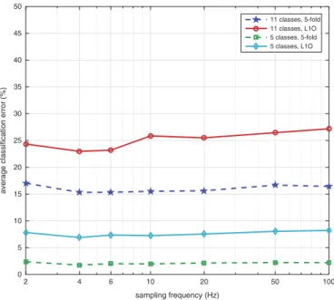
Figure 8.Effect of sampling frequency on the average classification error of thek-NN classifier (classifier 6).
0.2 0.3 0.4 0.5 0.7 1 0 5 10 15 20 25 30 35 40 45 50 segment duration (s)
average classification error (%)
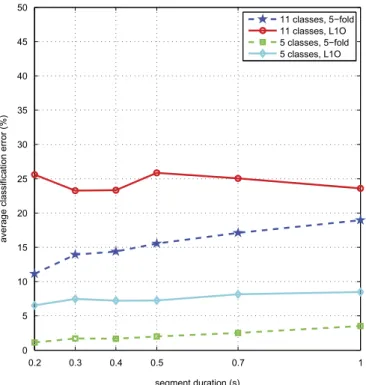
11 classes, 5−fold 11 classes, L1O 5 classes, 5−fold 5 classes, L1O
Figure 9.Effect of segment duration on the average classification error of the k-NN classifier (classifier 6).
shape−preserving cubic−spline smoothing spline 0 5 10 15 20 25 30 35 40 45 50
curve fitting method
average classification error (%)
11 classes, 5−fold 11 classes, L1O 5 classes, 5−fold 5 classes, L1O
Figure 10.Effect of curve-fitting method on the average classification error of thek-NN classifier (classifier 6).
equal priors priors from class freq. 0 5 10 15 20 25 30 35 40 45 50 prior probabilities
average classification error (%)
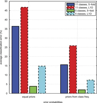
11 classes, 5−fold 11 classes, L1O 5 classes, 5−fold 5 classes, L1O
Figure 11.Effect of prior probabilities on the average classification error of the k-NN classifier (classifier 6). 1235710 20 30 40 50 70 100 168* 0 5 10 15 20 25 30 35 40 45 50
dimension of the reduced space (*: without feature reduction)
average classification error (%
) 11 classes, 5−fold 11 classes, L1O 5 classes, 5−fold 5 classes, L1O 1 2 3 4 6 8 10 0 5 10 15 20 25 30 35 40 45 50
dimension of the reduced space
average classification error (%
)
11 classes, 5−fold 11 classes, L1O 5 classes, 5−fold 5 classes, L1O
Figure 12.Effect of feature reduction with (a) PCA and (b) LDA on the average classification error of thek-NN classifier (classifier 6).
complete and simplified classification problems (a total of four cases). All the error percentage values presented in these figures are the average values over the five executions. Because the k-NN classifier outperforms all the other classifiers, the average classification error of only this classifier is shown in the figures. As expected, the 11-class classification problem results in larger errors compared to the 5-class problem. From the results, it can be observed that in all cases, 5-fold cross validation provides better results than subject-based L1O. This is because in the first case, the system is trained and tested with a random mixture of different subjects’ data, whereas in the second, it is trained with four subjects’ data and tested with the data of the remaining subject, who is totally new to the system.
Effect of sampling frequency (fs)
When the sampling frequency is set quite low, in particular, between 2–6 Hz, classification accuracy is acceptable. This occurs because people move rela-tively slowly and classification performance does not degrade much when the high-frequency components are removed.
The average classification error increases slightly with an increasing
sam-pling rate (Figure 8). For instance, with fs = 100 Hz, noting that the
dimen-sion of the feature space also increases with the number of samples in a segment, the data become so complicated that it misleads most of the classifiers. This is because the position measurements are quite noisy; hence, selecting a high sampling rate might cause overfitting, which degrades classification accuracy. We determine 10 Hz to be a suitable value for fs and set it as the default value.
Effect of segment duration (frm_dur)
Because a single event or activity is associated with each segment, the segment duration is another parameter that affects accuracy. Results for
segment duration values between 0.2 s and 1 s are shown in Figure 9.
Although the smallest segment duration usually gives slightly better results, the system must make a decision five times per second with this duration, which increases complexity. In fact, even a segment con-sisting of a single position measurement (one row of the dataset) is sufficient to obtain body posture information because it directly provides the 3D positions of the tags on different body parts at that instant. Compromising between complexity and accuracy, we select a segment duration of 0.5 s as the default value without much loss in classification accuracy in any of the four cases.
Effect of curve-fitting algorithm
From Figure 10, we observe that the shape-preserving and cubic-spline interpolations provide very similar results. Smoothing-spline interpolation performs the best among the three for 5-fold cross validation with 11 classes, whereas it performs the worst in the other three cases. Thus, the shape-preserving interpolation is chosen as the default curve-fitting method.
Effect of prior probabilities
Classification errors for individual classes can be obtained from the
confu-sion matrices provided inTables 2and 3. The average probability of error is
calculated by weighting the classification error of each class with its prior probability. In this study, we chose prior class probabilities in two different ways. In the first, prior probabilities are taken equally for each class, whereas in the second, prior probabilities are set equal to the actual occurrence of the
classes in the data.Figure 11illustrates the effect of prior probabilities on the
average classification error; the error for the case with equal priors is larger because transition classes (“Segmentation”) rarely occur in the dataset, thus their probability of occurrence is extremely low. However, the classification errors for these classes are larger because when a weighted average is calculated using the actual class probabilities, terms with large classification errors contribute relatively less to the total average error.
Effect of feature reduction
Because there is a large number of features (determined from the sampling frequency and the segment duration), two common methods (PCA and LDA) are used for feature reduction. All the results up to this point, includ-ing Figures 8–12, are obtained without feature reduction.
Figure 12(a)shows the average classification error when PCA is used with different reduced dimensionalities (from 1 to 100) as well without feature reduction (168). We observe that the intrinsic dimensionality of the feature vectors is about 10, which is much smaller than the actual dimension.
Figure 12(b) corresponds to the cases where LDA is used with reduced dimension from 1 to 10 for 11 classes and from 1 to 4 for 5 classes (note that reduced dimension must be lower than the number of classes in LDA). For the complete classification problem with 11 classes, LDA with dimension 10 outperforms all other cases, including those without feature reduction vali-dated by subject-based L1O. Including a large number of features not only increases the computational complexity of the system significantly, but also confuses the classifiers, leading to a less accurate system (this is well-known
For the 11-class problem, LDA with dimension 10 performs better than PCA when L1O is used and worse when 5-fold cross validation is employed. For the simplified problem with 5 classes, the results change similarly with feature reduction. With subject-based L1O, LDA with dimension 4 outper-forms PCA with higher dimensions as well as the case without feature reduc-tion. When 5-fold cross validation is used, PCA with dimension 20 is the best. Hence, LDA with dimension 4 is preferable because its performance seems to be less dependent on the subject performing the activities. Therefore, it can be stated that LDA is more reliable if the system is going to be used with subjects who are not involved in the training process. On the other hand, if the system is going to be trained for each subject separately, PCA results in a more accurate classifier, even at the same dimensionality as LDA.
Summary and conclusions
In this study, we present a novel approach to human activity recognition using a tag-based RF localization system. Accurate activity recognition is achieved without needing to consider the subject’s interaction with objects in his/her environment. In this scheme, subjects wear four RF tags whose positions are measured via multiple antennas (readers) fixed to the environment.
The most important issue in the scheme is the asynchronous and nonuniform acquisition of position data. The system records measure-ments whenever it detects a tag, and detection frequency is affected by the SNR and interference in the environment. The asynchronous nature of the data acquired introduces some additional problems to be tackled; for example, only one tag can be detected at a given time instant. Hence, the measurements of different tags are acquired at different time instants in a random manner. We solved this problem by first fitting a suitable curve to each measurement axis along time, and then resampling the fitted curves uniformly at a higher sampling rate at exactly the same time instants.
After the uniformly sampled curves are obtained, they are partitioned into segments of maximum duration of one second each, such that each segment is associated with only one activity. Then, various features are extracted from the segments for the classification process. The number of features is reduced using two feature reduction techniques.
We investigate ten different classifiers and calculate their average classifi-cation errors for various curve-fitting and feature reduction techniques and system parameters. We use two cross-validation methods, namely P-fold with P = 5, and subject-based L1O. Omitting the transition classes, the complete pattern recognition problem with 11 classes is reduced to a problem with five classes and the whole process is repeated. Finally, for each problem and for
each cross-validation method, we present the set of parameters and the classifier with the best result.
For the complete problem with 11 classes, the proposed system has an average classification error of 8.67% and 21.30% for the 5-fold and subject-based L1O cross-validation techniques, respectively. This relatively large error is caused by transition activities, which, with their shorter duration and fewer samples, are more difficult to recognize. When these activities are discarded, the reduced system with five classes has an average probability of error of 1.12% and 6.52% with 5-fold and subject-based L1O cross validation, respectively. Hence, performance significantly improves when transition activities are removed, as expected. The system proposed here demonstrates acceptable performance for most practical applications.
In future work, activity recognition by tracking body movement can be explored using asynchronously and nonuniformly acquired RFID data in raw form. Features can be directly calculated from the nonuniformly acquired samples with special techniques and then classified. HMMs can be used for accurately spotting activities and detecting the transition instants. Variable segment durations that are truncated at activity transi-tion points can then be considered. The set of activities can be broadened and activity and location information can be combined to provide more accurate results.
References
Aggarwal, J. K., and Q. Cai. 1999. Human motion analysis: A review. Computer Vision and Image Understanding 73 (3):428–440. doi:10.1006/cviu.1998.0744.
Alfaro, C. A., B. Aydın, C. E. Valencia, E. Bullitt, and A. Ladha. 2014. Dimension reduction in principal component analysis for trees. Computational Statistics & Data Analysis 74 (June):157–179. doi:10.1016/j.csda.2013.12.007.
Altun, K., and B. Barshan. 2010. Human activity recognition using inertial/magnetic sensor units. In Human behavior understanding (HBU 2010), LNCS, ed. A. A. Salah et al., vol. 6219, 38–51. Berlin, Heidelberg: Springer.
Altun, K., and B. Barshan. 2012. Pedestrian dead reckoning employing simultaneous activity recognition cues. Measurement Science and Technology 23 (2):025103. doi:
10.1088/0957-0233/23/2/025103.
Altun, K., B. Barshan, and O. Tunçel. 2010. Comparative study on classifying human activities with miniature inertial and magnetic sensors. Pattern Recognition 43 (10):3605– 3620. doi:10.1016/j.patcog.2010.04.019.
Ayrulu-Erdem, B., and B. Barshan. 2011. Leg motion classification with artificial neural networks using wavelet-based features of gyroscope signals. Sensors 11 (2):1721–1743.
doi:10.3390/s110201721.
Barshan, B., and M. C. Yüksek. 2014. Recognizing daily and sports activities in two open source machine learning environments using body-worn sensor units. The Computer Journal 57 (11):1649–1667. doi:10.1093/comjnl/bxt075.
Barshan, B., and A. Yurtman. 2016. Investigating inter-subject and inter-activity variations in activity recognition using wearable motion sensors. The Computer Journal, [online]
doi:10.1093/comjnl/bxv093.
Bicocchi, N., M. Mamei, and F. Zambonelli. 2010. Detecting activities from body-worn accelerometers via instance-based algorithms. Pervasive and Mobile Computing 6 (4):482–495. doi:10.1016/j.pmcj.2010.03.004.
Bouet, M., and A. L. dos Santos. 2008. RFID tags: Positioning principles and localization techniques. Paper presented at The 1st IFIP Wireless Days Conference, 1–5, United Arab Emirates, November 24–27.
Buettner, M., R. Prasad, M. Philipose, and D. Wetherall. 2009. Recognizing daily activities with RFID-based sensors. Proceedings of the 11th International Conference on Ubiquitous Computing (UBICOMP 2009), 51–60, Orlando, FL, USA, September 30–October 3. Choi, B.-S., J.-W. Lee, and J.-J. Lee. 2008. Localization and map-building of mobile robot
based on RFID sensor fusion system. Proceedings of the 6th IEEE Conference on Industrial Informatics, 412–417, Daejeon, Korea, July 13–16.
Duda, R. O., P. E. Hart, and D. G. Stork. 2001. Pattern classification, (2nd ed.). Hoboken, NJ: John Wiley & Sons, Inc.
Duin, R. P. W., P. Juszczak, P. Paclik, E. Pekalska, D. de Ridder, D. M. J. Tax, and S. Verzakov. 2007. PRTools 4.1, A MATLAB toolbox for pattern recognition. The Netherlands: Delft University of Technology, version 4.1,http://www.prtools.org/(accessed February 2016). Duong, T. V., H. H. Bui, D. Q. Phung, and S. Venkatesh. 2005. Activity recognition and
abnormality detection with the switching hidden semi-Markov model. Proceedings of IEEE Computer Society Conference on Computer Vision and Pattern Recognition (CVPR 2005), vol. 1, 838–845, San Diego, CA, USA, June 20–25.
Feldhofer, M., S. Dominikus, and J. Wolkerstorfer. 2004. Strong authentication for RFID systems using the AES algorithm. In Cryptographic hardware and embedded systems, (CHES 2004), LNCS, ed. M. Joye and J.-J. Quisquater, vol. 3156/2004: 357–370. Berlin, Heidelberg: Springer.
Guenterberg, E., H. Ghasemzadeh, V. Loseu, and R. Jafari. 2009. Distributed continuous action recognition using a hidden Markov model in body sensor networks. In Distributed computing in sensor systems, LNCS, ed. B. Krishnamachari et al., vol. 5516/2009, 145–158. Berlin, Heidelberg: Springer. doi:10.1007/978-3-642-02085-8_11.
Hahnel, D., W. Burgard, D. Fox, K. Fishkin, and M. Philipose. 2004. Mapping and localiza-tion with RFID technology. Proceedings of the IEEE Internalocaliza-tional Conference on Robotics and Automation, vol. 1, 1015–1020, New Orleans, LA, USA, April 26–May 1.
Hapfelmeier, A., and K. Ulm. 2014. Variable selection by Random Forests using data with missing values. Computational Statistics & Data Analysis 80:129–139. doi:10.1016/j.
csda.2014.06.017.
Huang, P.-C., S.-S. Lee, Y.-H. Kuo, and K.-R. Lee. 2010. A flexible sequence alignment approach on pattern mining and matching for human activity recognition. Expert Systems with Applications 37 (1):298–306. doi:10.1016/j.eswa.2009.05.057.
Junker, H., O. Amft, P. Lukowicz, and G. Tröster. 2008. Gesture spotting with body-worn inertial sensors to detect user activities. Pattern Recognition 41 (6):2010–2024. doi:10.1016/
j.patcog.2007.11.016.
Kaluža, B., V. Mirchevska, E. Dovgan, M. Luštrek, and M. Gams. 2010. An agent-based approach to care in independent living. In Ambient intelligence, LNCS, ed. B. de Ruyter et al., vol. 6439/ 2010, 177–186. Berlin, Heidelberg: Springer. doi:10.1007/978-3-642-16917-5_18.
Kern, N., B. Schiele, and A. Schmidt. 2003. Multi-sensor activity context detection for wearable computing. In Ambient intelligence (EUSAI 2003), LNCS, ed. E. Aarts et al., vol. 2875, 220–232. Berlin, Heidelberg: Springer.
Liu, H., H. Darabi, P. Banerjee, and J. Liu. 2007. Survey of wireless indoor positioning techniques and systems. IEEE Transactions on Systems, Man and Cybernetics, Part C (Applications and Reviews) 37 (6):1067–1080. doi:10.1109/TSMCC.2007.905750.
Logan, B., J. Healey, M. Philipose, E. M. Tapia, and S. Intille. 2007. A long-term evaluation of sensing modalities for activity recognition. In UbiComp 2007: Ubiquitous computing, LNCS, ed. J. Krumm et al., vol. 4717, 483–500. Berlin, Heidelberg: Springer.
Luštrek, M., and B. Kaluža. 2009. Fall detection and activity recognition with machine learning. Informatica 33 (2):205–212.
Luštrek, M., B. Kaluža, E. Dovgan, B. Pogorelc, and M. Gams. 2009. Behavior analysis based on coordinates of body tags. In Ambient intelligence, LNCS, ed. M. Tscheligi et al., vol. 5859/2009, 14–23. Berlin, Heidelberg: Springer. doi:10.1007/978-3-642-05408-2_2. Mannini, A., and A. M. Sabatini. 2010. Machine learning methods for classifying human
physical activity from on-body accelerometers. Sensors 10 (2):1154–1175. doi:10.3390/
s100201154.
Marín-Jiménez, M. J., N. Pérez de la Blanca, and M. A. Mendoza. 2014. Human action recognition from simple feature pooling. Pattern Analysis and Applications 17 (1):17–36.
doi:10.1007/s10044-012-0292-8.
Mathie, M. J., A. C. F. Coster, N. H. Lovell, and B. G. Celler. 2004. Accelerometry: Providing an integrated, practical method for long-term, ambulatory monitoring of human move-ment. Physiological Measurement 25 (2):R1–R20. doi:10.1088/0967-3334/25/2/R01. MicroStrain. 2016. MicroStrain inclinometers and orientation sensors. Williston, VT USA:
MicroStrain,http://www.microstrain.com/3dm-gx2.aspx(accessed February 2016). Moeslund, T. B., A. Hilton, and V. Krüger. 2006. A survey of advances in vision-based human
motion capture and analysis. Computer Vision and Image Understanding 104 (2–3):90–126.
doi:10.1016/j.cviu.2006.08.002.
Ngai, E. W. T., K. K. L. Moon, F. J. Riggins, and C. Y. Yi. 2008. RFID research: An academic literature review (1995–2005) and future research directions. International Journal of Production Economics 112 (2):510–520. doi:10.1016/j.ijpe.2007.05.004.
Ni, L. M., Y. Liu, Y. C. Lau, and A. P. Patil. 2004. LANDMARC: Indoor location sensing using active RFID. Wireless Networks 10 (6):701–710. (Issue: Pervasive Computing and Communications). doi:10.1023/B:WINE.0000044029.06344.dd.
Ogris, G., P. Lukowicz, T. Stiefmeier, and G. Tröster. 2012. Continuous activity recognition in a maintenance scenario: Combining motion sensors and ultrasonic hands tracking. Pattern Analysis and Applications 15 (1):87–111. doi:10.1007/s10044-011-0216-z.
Özdemir, A. T., and B. Barshan. 2014. Detecting falls with wearable sensors using machine learning techniques. Sensors 14 (6):10691–10708. doi:10.3390/s140610691.
Philipose, M., K. P. Fishkin, M. Perkowitz, D. J. Patterson, D. Fox, H. Kautz, and D. Hahnel. 2004. Inferring activities from interactions with objects. IEEE Pervasive Computing 3 (4):50–57. doi:10.1109/MPRV.2004.7.
Sabatini, A. M. 2006. Inertial sensing in biomechanics: A survey of computational techniques bridging motion analysis and personal navigation. In Computational intelligence for move-ment sciences: Neural networks and other emerging techniques, ed. R. K. Begg and M. Palaniswami, 70–100. Hershey, PA: Idea Group Publishing. doi:
10.4018/978-1-59140-836-9.ch002.
Smith, J. R., K. P. Fishkin, B. Jiang, A. Mamishev, M. Philipose, A. D. Rea, S. Roy, and K. Sundara-Rajan. 2005. RFID-based techniques for human-activity detection. Communications of the ACM 48 (9):39–44. (Special Issue: RFID). doi:10.1145/1081992. Steggles, P., and S. Gschwind. 2005. The Ubisense smart space platform, Technical Report,
Stikic, M., T. Huynh, K. van Laerhoven, and B. Schiele. 2008. ADL recognition based on the combination of RFID and accelerometer sensing. Proceedings of the 2nd International Conference on Pervasive Computing Technologies for Healthcare, 258–263, Tampere, Finland, January 30–February 1.
Sukthankar, G., and K. Sycara. 2005. A cost minimization approach to human behavior recognition. Proceedings of the 4th International Joint Conference on Autonomous Agents and Multiagent Systems (AAMAS 2005), 1067–1074, Utrecht, Netherlands, July 25–29. SYRIS Technology Corp. (The RFID Total Solution). 2016. Address: 12F., No.16, Sec. 2,
Taiwan Blvd., West Dist., Taichung City 403, Taiwan.http://www.syris.com.
Tapia, E. M., S. S. Intille, and K. Larson. 2004. Activity recognition in the home using simple and ubiquitous sensors. In Pervasive computing (PERVASIVE 2004), LNCS, ed. A. Ferscha, and F. Mattern, vol. 3001/2004, 158–175. Berlin, Heidelberg: Springer.
Tunçel, O., K. Altun, and B. Barshan. 2009. Classifying human leg motions with uniaxial piezoelectric gyroscopes. Sensors 9 (11):8508–8546. doi:10.3390/s91108508.
University of California, Irvine, Machine Learning Repository. 2010. Localization data for person activity data set. http://archive.ics.uci.edu/ml/datasets/Localization+Data+for
+Person+Activity.
Wang, L., T. Gu, X. Tao, and J. Lu. 2009. Sensor-based human activity recognition in a multiuser scenario. In Ambient intelligence, LNCS, ed. M. Tscheligi et al., vol. 5859/2009, 78–87. Berlin, Heidelberg: Springer. doi:10.1007/978-3-642-05408-2_10.
Wang, L., W. Hu, and T. Tan. 2003. Recent developments in human motion analysis. Pattern Recognition 36 (3):585–601. doi:10.1016/S0031-3203(02)00100-0.
Want, R. 2006. An introduction to RFID technology. IEEE Pervasive Computing 5 (1):25–33.
doi:10.1109/MPRV.2006.2.
Weis, S. A. 2012. RFID (Radio-Frequency Identification). In Handbook of Computer Networks: Distributed Networks, Network Planning, Control, Management, and New Trends and Applications, vol. 3 (ed H. Bidgoli), Chapter 63, Hoboken, NJ: John Wiley & Sons, Inc. doi:10.1002/9781118256107.ch63.
Welch, G., and E. Foxlin. 2002. Motion tracking: No silver bullet, but a respectable arsenal. IEEE Computer Graphics and Applications 22 (6):24–38. doi:10.1109/MCG.2002.1046626. Wong, W. Y., M. S. Wong, and K. H. Lo. 2007. Clinical applications of sensors for human
posture and movement analysis: A review. Prosthetics and Orthotics International 31 (1):62–75. doi:10.1080/03093640600983949.
Wu, J., A. Osuntogun, T. Choudhury, M. Philipose, and J. M. Rehg. 2007. A scalable approach to activity recognition based on object use. Proceedings of the IEEE 11th International Conference on Computer Vision, Rio de Janeiro, Brazil, October 14–20. Xsens Technologies B. V. 2016. MTi and MTx user manual and technical documentation
Enschede, The Netherlands: Xsenshttp://www.xsens.com. (accessed February 2016). Yue, D., X. Wu, and J. Bai. 2008. RFID application framework for pharmaceutical supply
chain. Proceedings of the IEEE International Conference on Service Operations and Logistics, and Informatics, vol. 1, 1125–1130, Beijing, China, October 12–15.
Yurtman, A., and B. Barshan. 2014. Automated evaluation of physical therapy exercises using multi-template dynamic time warping on wearable sensor signals. Computer Methods and Programs in Biomedicine 117 (2):189–207. doi:10.1016/j.cmpb.2014.07.003.
Zhang, Y., M. G. Amin, and S. Kaushik. 2007. Localization and tracking of passive RFID tags based on direction estimation. International Journal of Antennas and Propagation 2007 (article no: 17426):1–9. doi:10.1155/2007/17426.
Zijlstra, W., and K. Aminian. 2007. Mobility assessment in older people: New possibilities and challenges. European Journal of Ageing 4 (1):3–12. doi:10.1007/s10433-007-0041-9.