Full Terms & Conditions of access and use can be found at
http://www.tandfonline.com/action/journalInformation?journalCode=raec20
Download by: [Bilkent University] Date: 09 November 2017, At: 05:28
Applied Economics
ISSN: 0003-6846 (Print) 1466-4283 (Online) Journal homepage: http://www.tandfonline.com/loi/raec20
The Fisher hypothesis: a multi-country analysis
Hakan Berument & Mohamed Mehdi Jelassi
To cite this article: Hakan Berument & Mohamed Mehdi Jelassi (2002) The Fisher hypothesis: a multi-country analysis, Applied Economics, 34:13, 1645-1655, DOI: 10.1080/00036840110115118 To link to this article: http://dx.doi.org/10.1080/00036840110115118
Published online: 04 Oct 2010.
Submit your article to this journal
Article views: 132
View related articles
The Fisher hypothesis: a multi-country
analysis
H A K A N B E R U M E N T * and M O H A M E D M E H D I J E LA S S I
Department of Economics, Bilkent University, Ankara, Turkey
This paper tests whether the Fisher hypothesis holds for a sample of 26 countries by assessing the long run relationship between nominal interest rates and in¯ation rates taking into consideration the short run dynamics of interest rates. The empirical evidence supports the hypothesis that there is a one-to-one relationship between the interest rate and in¯ation for more than half of the countries under study.
I . I N T R O D U C T I O N
The Fisher hypothesis suggests that there is a positive rela-tionship between interest rates and expected in¯ation. Boudoukh and Richardson (1993) argue that this positive relationship exists at all horizon lengths. In contrast, Mishkin (1992) reported the presence of this relationship for the long-run, but he could not detect the presence of the Fisher e ect in the short-run for the USA. Moreover, Yuhn (1996) reported that the Fisher e ect is strong over long horizons, and the presence of the Fisher e ect can be seen in the short-run for Germany. Therefore, the results obtained by testing for the Fisher hypothesis might be in¯uenced by the time horizon that has been selected. This study tests the Fisher hypothesis within the frame-work suggested by Moazzami (1989), which allows a direct estimate of the long-run relationship between interest rates and expected in¯ation by taking into consideration the short-run dynamics of the interest rates for 26 developed and developing countries.
The contribution of this paper to the literature can be highlighted within the following four headings. First, to the best of the authors’ knowledge, this study is the most extensive study testing the Fisher hypothesis as far as the number of the countries that are incorporated is con-cerned.1 Second, the sample includes both developed and developing economies, hence this allows one to assess the presence of the Fisher hypothesis for two types of econo-mies. Third, studies that attempt to extract the long-term
e ect by applying methods similar to this utilized annual data (see Carmichael and Stebbing, 1983; Moazzami and Gupta, 1995), while this study uses monthly data. This is important because using annual data may lead to the aggregation biased problem suggested by Rossana and Seater (1995), whereas using monthly data may avoid that problem. Lastly, to the best of the authors’ knowledge, this paper reports the most comprehensive robustness tests among the studies on the Fisher hypothesis testing. The next section introduces the basic model that is used to test the Fisher hypothesis, Section III presents the empiri-cal evidence and Section IV summarizes the conclusions.
I I . TH E BA S I C M O D EL
The basic equation that has been used to test the Fisher hypothesis is
itˆ ¬ ‡ ºet …1†
Where it is the nominal interest rate and ºet is the expected in¯ation for the period t. Here, is expected to be one as there is a one-to-one relationship between interest rates and the expected in¯ation ± the strong form of the Fisher hypothesis. However, is positive but not equal to one in its weak form. Tobin (1965) suggests that if money and capital are the only forms of wealth, when the oppor-tunity cost of holding money increases due to higher in¯a-tion, money holding decreases and capital stock increases.
Applied Economics ISSN 0003±6846 print/ISSN 1466±4283 online # 2002 Taylor & Francis Ltd
http://www.tandf.co.uk/journals DOI: 10.1080 /0003684011011511 8
1645
* Corresponding author. E-mail:[email protected].
1Engsted (1995) and Koustas and Sertelis (1999) are the most comprehensive studies as far as the number of countries are concerned. These studies consider 13 and 11 OECD countries, respectively, for the testing of the Fisher hypothesis.
Under decreasing return to scale economies, then interest rate decreases with lower levels of marginal productivity of capital. Therefore, in Tobin’s world, should be positive and less than one ± the weak form of the Fisher hypothesis. On the other hand, tax-e ect suggests that is greater than one. Darby (1975) notes that when the nominal interest rate is taxed, the Fisher relationship implies that the change in the nominal interest rates is greater than the change in expected in¯ation so as to maintain the constant ex-ante real interest rate (see Crowder and Wodar, 1999). Nevertheless, all forms of Fisher hypothesis speci®cations suggest that is positive.
In order to test the Fisher hypothesis, Moazzami (1989) assumes that the economy is in a steady state equilibrium and there is no deviation from its long-run equilibrium path in the short run. Here, ignoring the short-run dynamics and simply regressing nominal interest rates against the current rate of in¯ation su ers from misspeci-®cation, which manifests itself in residual autocorrelation. In fact, the estimated results reported by Equation 1 are associated with a common characteristic that is displayed in a low Durbin±Watson statistic, which can be regarded as a speci®c error due to the omission of the short-run dynamics. Some studies have addressed this issue by using the Cochrane±Orcutt procedure: e.g. Tanzi (1980) and Carmichael and Stebbing (1983). Others have attempted to minimize the e ects of shorter-term ¯uctua-tions in the data, performing several transformation s to re¯ect only the long-run tendencies of the data: e.g. Lucas (1980) and Lothian (1985). However, by using these transformations , all the information on the short-run dynamics could be lost.
In order to incorporate the short-run dynamics of inter-est rates, Moazzami (1989) allows for the presence of lags of interest rates on the right hand side of the equation. Hence, Equation 1 is respeci®ed as:
itˆ ¬ ‡ Xm
iˆ1
³iit¡i‡ ºet‡ "t …2† In order to estimate Equation 2, the expected in¯ation rate ºet must be speci®ed. Gordon (1971) and Lahiri (1976) sug-gest that the expected in¯ation rate, which is unobservable, may be systematically related to past rates of in¯ation.2 Hence, using the distributed lag of past rates of in¯ation as a proxy for the expected rate of in¯ation, Equation 2 can be written as: itˆ ¬ ‡ Xm iˆ1 ³iit¡i‡ Xn iˆ0 ¶iºt¡i‡ et …3†
Moazzami (1989) argues that the coe cients of the lagged variables are, in general, signi®cantly di erent from zero in estimating Equation 3. In fact, if the coe -cients of all lagged variables in Equation 3 are set to be equal to zero, then the conventional Fisher equation esti-mation is obtained under the implicit assumption of a steady state equilibrium in which all expectations are rea-lized and the actual and expected rates of in¯ation are identical. In order to measure the expected in¯ation rate, an auxiliary equation can be used. However, using a dis-tributed lag of the actual in¯ation rates as a proxy for the expected rate has the advantage of avoiding the problems associated with the use of generated regressors. Under the assumption of no autocorrelation, Equation 3 can be esti-mated by using the Ordinary Least Squares (OLS) method. The estimates then give the long-run response coe cient of the interest rate to the rate of in¯ation. This is expressed as follows:
¡ˆ Pn
iˆ0¶i
1 ¡Pmiˆ1³i …4†
In order to calculate the variance of ¡ estimate, the trans-formation ®rst proposed by Bewley (1979) and then modi-®ed by Wickens and Breusch (1988) was used. The method ®rst subtracts …Pmiˆ1³i†itfrom each side of Equation 3 and rearranges the terms such that it yields:
itˆ ¬ ¡ £ X m¡1 iˆ0 Xm jˆi‡1 ³j Á ! ¢it¡i‡ £ X n iˆ0 ¶i Á ! ºt ¡ £X n¡1 iˆ0 Xn jˆi‡1 ¶j Á ! ¢ºt¡i‡ £et …5† where
¢Xt¡i ˆ Xt¡i¡ Xt¡i¡1
£ˆ 1
1 ¡Pmiˆ1³i
Here, the coe cient of ºtis the long-run multiplier of the Fisher equation, ¡, as de®ned in Equation 4. The long-run adjustment coe cient for the interest rate, as well as the other coe cients of Equation 5, can be estimated using the instrumental variable method. Wickens and Breusch (1988) showed that the estimate of the long-run multiplier obtained by estimating the transformed model, Equation 5 via instrumental variables is numerically identical to the one calculated from the OLS estimates of Equation 3, pro-vided that all the predetermined variables of the original Equation 3 are used as instruments. Hence, this paper esti-mates the form of Equation 5 with the instrumental
vari-2In addition to using the autoregressive speci®cation of the in¯ation equation, other speci®cations are tried, such as including the lag and (or) current values of money growths to form the expectations of the in¯ation for some of the countries. When these alternative speci®cations are used, the basic results of the study were robust.
able technique in order to test the basic implication of the Fisher hypothesis.
I I I . R E S U L T S
This section presents the basic empirical evidence for test-ing the Fisher hypothesis. The next sub-section introduces the data, the second sub-section reports the estimates of the model, the third sub-section is for the robustness analyses.
Data
Interest data is either treasury bill rates, if available, or the lending rate. The lending rate, rather than other interest rates, is used when the treasury bill rate is not available because it is believed that the lending rate is the most risk free measure of interest rates after treasury bill rates. The in¯ation rate is measured by the logarithmic ®rst di erence of the consumer price index. The countries that were ex-amined, the de®nition of the interest rate that was used and the data sample are reported in Table 1. All the data are from the International Monetary Fund±International
Financial Statistics tape and the sample size is the largest monthly sample that is available from the tape. The speci®c de®nitions of treasury bill and lending rates for each coun-try are also available from the tape.
Estimates and basic results
In order to estimate Equation 5, the optimum lag orders of the interest rate and in¯ation are determined from Equation 3. In order to determine the optimum lag orders for lagged values of both in¯ation and interest rates, the Final Prediction Error Criteria suggested by Hsiao (1979) is used. His method determines the optimum lag order such that the residual term is no longer autocorrelated. Once the optimum lag length is determined, these lag orders are used as the lag orders of those two variables in Equation 5.
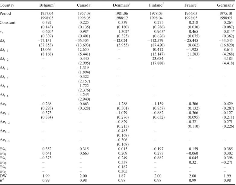
In order to assess the short- and long-run dynamics of interest rates, Equation 5 is estimated via the instrumental variable method, where the predetermined variables of Equation 3 are used as instruments [parallel to those pro-posed by Wickens and Breusch (1988)]. This method allows one to estimate the long-run adjustment coe cient, ¡, for the interest rate to the rate of in¯ation directly. The esti-mates of the model for the developed countries under study are reported in Table 2, and Table 3 reports the estimates for developing countries.
For the 26 countries examined, except for Brazil and Costa Rica, positive coe cients are estimated for ¡. The null hypothesis that ¡ is one ± the strong version of the Fisher hypothesis ± is also tested. The test statistics could not reject the null hypothesis for 16 out of 26 countries. Among the developed countries, no evidence was found to reject the strong version of the Fisher hypothesis for 9 out of 12 countries; these countries are Belgium, Canada, Denmark, Finland, Germany, Italy, Japan, Switzerland and the USA. However, the estimated coe cients of ¡ for Belgium and Finland are not statistically signi®cantly di erent from zero. The results in the strong form of the Fisher hypothesis are in line with those reported by Moazzami and Gupta (1995) for Canada, Germany, Italy, the UK and the USA. The only result of the study con¯icting with that of Moazzami and Gupta (1995) is in the case of France. One possible reason for the di erence is that they used annual data from 1953 to 1989 and this study used monthly data from 1966:03 to 1998:05. For the twelve developed countries that have been examined in this study, the authors tested whether the coe cient of the in¯ation, ¡, is positive and statistically signi®cant among the countries where the strong form of the Fisher hypothesis is rejected. Only the null hypothesis that ¡ is zero, the weak form of the Fisher hypothesis, for France is rejected. Only for the UK is the coe cient not statistically signi®cant.
The Fisher hypothesis is tested for the set of the devel-oping countries and the results are reported in Table 3. No
Table 1. List of countries studied
Country Interest rate used Sample period Developed countries
Belgium Treasury bill rate 1957:04 1998:05 Canada Treasury bill rate 1957:08 1998:05 Denmark Treasury bill rate 1981:06 1988:12
Finland Lending rate 1978:03 1998:04
France Treasury bill rate 1966:03 1998:05 Germany Treasury bill rate 1975:10 1998:05 Italy Treasury bill rate 1977:07 1998:04
Japan Lending rate 1957:05 1998:05
Korea Lending rate 1981:01 1998:03
Switzerland Treasury bill rate 1980:05 1998:05 UK Treasury bill rate 1964:07 1998:05 USA Treasury bill rate 1964:04 1998:05
Developing countries
Brazil Treasury bill rate 1995:05 1998:03
Chile Lending rate 1978:01 1998:05
Costa Rica Lending rate 1982:05 1998:05
Egypt Lending rate 1976:03 1998:04
Greece Lending rate 1957:05 1998:05
India Lending rate 1979:04 1998:01
Kuwait Treasury bill rate 1979:08 1996:07 Mexico Treasury bill rate 1978:04 1998:05 Morocco Treasury bill rate 1978:08 1991:12 Philippines Treasury bill rate 1982:01 1998:04 Turkey Treasury bill rate 1985:12 1995:08
Uruguay Lending rate 1980:04 1998:05
Venezuela Lending rate 1984:07 1998:04 Zambia Treasury bill rate 1985:02 1998:01
statistically signi®cant evidence was found to reject the strong version of the Fisher hypothesis for 7 out of 14 countries: Chile, Greece, Mexico, Turkey, Uruguay, Venezuela and Zambia. The empirical evidence also sug-gests that among the countries where the strong form of the Fisher hypothesis is not supported (Brazil, Costa Rica, Egypt, India, Kuwait, Morocco and the Philippines), the null hypothesis that ¡ is zero for Brazil, Costa Rica, India, Kuwait and Morocco could not be rejected. For the Mexican case, the result is parallel with the result reported by Thornton (1996).
The short-run dynamics of the nominal interest rate to the expected in¯ation rate are reported in Tables 2 and 3. £¶0, £¶1, £¶2; . . . ; £¶5 show the response of the nominal interest rate to expected in¯ation in the corresponding per-iod. Examining the countries where the strong form of the Fisher hypothesis holds, it is concluded that the short-run
responses of the nominal interest rate to expected in¯ation do not display a consistent pattern. In fact, the adjustment process di ers from one country to another. However, an interesting point is that for some of the developing coun-tries, the short-run adjustment of the nominal interest rate to expected in¯ation is more than proportional, in particu-lar for the Chilean, Mexican and Venezuelan cases. In con-trast, for the developed countries, the short-run adjustment of the nominal rate to expected in¯ation is always less than proportional.
Robustness analyses
It is possible that the regression analyses performed in the last section give spurious regression results. Hence, in this section various robustness tests are performed. First, the errors of the model are tested for autocorrelation. These
Table 2. Long-term e ect of in¯ationary expectatons on the nominal interest rate: developed countries
Country Belgiumt Canadat Denmarkt Finlandl Francet Germanyt
Period 1957:04 1957:08 1981:06 1978:03 1966:03 1975:10 1998:05 1998:05 1988:12 1998:04 1998:05 1998:05 Constant 0.392 0.225 0.339 0.275 0.218 0.264 (0.143) (0.135) (0.180) (0.286) (0.030) (0.087) ºt 0.620* 0.98* 1.302* 0.963* 0.465 0.814* (0.339) (0.401) (0.325) (0.626) (0.075) (0.362) ¢it ¡77.131 ¡36.305 ¡12.024 ¡112.579 ¡25.445 ¡33.545 (37.853) (13.693) (5.955) (87.420) (8.662) (16.820) ¢it¡1 13.066 12.650 ± 10.412 ¡1.925 8.613 (8.168) (5.441) (15.147) (1.283) (4.268) ¢it¡2 ± 0.440 ± 23.684 ± 4.183 (2.995) (17.888) (4.418) ¢it¡3 ± ¡1.319 ± ± ± ± (1.894) ¢it¡4 ± ¡0.322 ± ± ± ± (2.157) ¢it¡5 ± 1.722 ± ± ± ± (2.376) ¢it¡6 ± ¡4.245 ± ± ± ± (2.940) ¢ºt ¡0.268 ¡0.663 ¡1.288 ¡1.159 ¡0.306 ¡0.429 (0.293) (0.328) (0.301) (0.857) (0.132) (0.287) ¢ºt¡1 0.373 ± ¡1.079 ¡0.882 ¡0.366 ¡0.127 (0.384) (0.276) (0.632) (0.095) (0.211) ¢ºt¡2 ± ± ¡0.829 ± ¡0.321 0.271 (0.215) (0.110) (0.226) ¢ºt¡3 ± ± ¡0.483 ± ± (0.168) ¢ºt¡4 ± ± ¡0.306 ± ± ± (0.168) £¶0 0.352 0.315 0.015 ¡0.197 0.159 0.385 £¶1 0.641 0.663 0.209 0.277 ¡0.060 0.302 £¶2 ¡0.373 ± 0.249 0.882 0.045 0.398 £¶3 ± ± 0.337 ± 0.321 ¡0.271 £¶4 ± ± 0.187 ± ± ± £¶5 ± ± 0.305 ± ± ± DW 1.99 2.00 1.87 2.00 2.00 1.99 R2 0.99 0.98 0.98 0.98 0.99 0.98
error terms are then tested for the autoregressive con-ditional heteroscedasticity (ARCH) by using the ARCH-LM test suggested by Engle (1982). Lastly, stability tests using Chow’s test are performed.
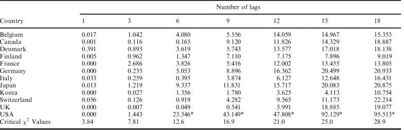
Tables 4 and 5 report the Ljung-Box Q statistics for serial correlations for di erent lag orders for all the coun-tries under study. Table 4 suggests that the autocorrelation problem is not present for any of the developed countries except for the USA. The Fisher hypothesis estimates for the USA are addressed later in the paper. Table 5 reports the Q-statistics for the developing countries under study. The null hypothesis of no autocorrelation is rejected only in the Zambia case for the 15th and 18th lags and in the Chile case for the 12th lag. The autocorrelation problem
for those two developing economies exists only in high orders; therefore, it is assumed that the autocorrelation problem does not exist for these countries.
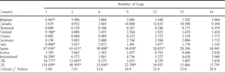
As a second test of robustness, ARCH-LM tests are performed in order to check for the presence of the ARCH e ect. Therefore, the model’s squared residuals are regressed on its lagged squared residuals in di erent lag orders and the constant term in order to test the null hypothesis that the coe cient of the lagged squared resi-duals are all zero. Table 6 and Table 7 report the calculated
F-statistics for each country under study and for the di
er-ent number of squared residual lags. Table 6 reports the ARCH-LM test for the developed economies in the sample. The test statistics could not reject the null hypothesis that
Table 2. (continued)
Country Italyt Japanl Koreal Switzerlandt UKt USAt
Period 1977:07 1957:05 1981:01 1980:05 1964:07 1964:04 1998:04 1998:05 1998:03 1998:05 1998:05 1998:05 Constant 0.470 0.352 0.729 0.189 0.686 0.276 (0.180) (0.196) (0.070) (0.068) (0.101) (0.127) ºt 0.744* 0.430* 0.339 0.661* 0.113 0.663* (0.223) (0.302) (0.204) (0.306) (0.124) (0.401) ¢it ¡27.378 ¡262.474 ¡21.695 ¡18.979 ¡34.903 ¡23.106 (13.104) (173.425) (9.419) (7.930) (11.997) (12.678) ¢it¡1 ¡0.152 177.103 3.561 1.069 13.819 8.274 (2.467) (116.483) (3.542) (1.725) (5.542) (5.527) ¢it¡2 3.469 ¡57.148 ¡1.084 1.730 ¡1.023 ¡5.331 (2.838) (51.079) (1.373) (1.697) (2.125) (4.323) ¢it¡3 0.369 79.175 6.111 2.775 ¡0.351 ± (2.199) (47.731) (3.488) (2.067) (2.273) ¢it¡4 ± ± 0.517 ± 0.021 ± (1.581) (2.294) ¢it¡5 ± ± ± ± 2.507 ± (2.187) ¢ºt ¡0.974 ¡0.210 ± ¡0.770 ¡0.253 0.081 (0.397) (0.161) (0.295) (0.119) (0.413) ¢ºt¡1 ± ± ± ¡0.269 ¡0.203 0.396 (0.184) (0.106) (0.417) ¢ºt¡2 ± ± ± ± ± ¡0.173 (0.307) ¢ºt¡3 ± ± ± ± ± 0.049 (0.356) ¢ºt¡4 ± ± ± ± ± ¡0.909 (0.483) £¶0 ¡0.230 0.220 0.339 ¡0.109 ¡0.140 0.744 £¶1 0.974 0.210 ± 0.501 0.049 0.315 £¶2 ± ± ± 0.269 0.203 ¡0.569 £¶3 ± ± ± ± ± 0.222 £¶4 ± ± ± ± ± ¡0.959 £¶5 ± ± ± ± ± 0.909 DW 2.02 1.99 1.99 2.02 1.99 2.00 R2 0.97 0.99 0.96 0.96 0.97 0.96
Standard deviations are given in parentheses.
Standard deviations are corrected for heteroscedasticity with White (1980). * Do not reject the null hypothesis: ¡ ˆ 1 at the 5% signi®cance level.
tTreasury bill rate is used to model the interest rate. l
Lending rate is used to model the interest rate.
there is no ARCH e ect for Canada, Denmark, France, Germany and Korea. For the Belgian, Finnish, Italian and Swiss speci®cations, autoregressive conditional heterosce-dasticity is detected only for one lag of the squared resi-duals. However, for the USA and Japan, autoregressive conditional heteroscedasticit y is detected for most of the lags of the squared residuals included. Table 7 reports the ARCH-LM tests for the set of developing countries. The test statistics cannot reject the null hypothesis that there is no autoregressive conditional heteroscedasticity for any of the countries in the sample except for the cases of Chile, Turkey and Venezuela. In the case of Turkey, the ARCH process is detected only when one lag of the squared resi-duals is included. For Chile and Venezuela, however, the ARCH process is detected when one and three lags of the squared residuals are included. To sum up, of all the coun-try models that were estimated, the ARCH e ect has been defected only for Belgium, Chile, Finland, Italy, Japan, Switzerland, Turkey, the UK, the USA and Venezuela out of the 26 countries in the sample. In this study, the presence of the ARCH e ect may indicate the presence of the misspeci®cation as well as the presence of the time varying risk in the interest rates. Further research is needed
to elaborate upon this issue; hence, it is left for a further study.
As a third robustness test in addition to testing the mod-els for any serial autocorrelation and for the ARCH e ect, models were tested for possible structural changes. The empirical evidence suggests that none of the countries except for the USA indicate structural change at the con-ventional 5% level (results are not reported here, but are available from the authors upon request).
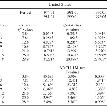
In order to address the structural change for the US speci®cation, the model is reestimated for di erent sub-samples as suggested by the Chow break-point tests. The estimates are provided in Table 8. Even if none of the coe cients of the in¯ation are statistically signi®cant, the Fisher hypothesis in its strong form could not be rejected for any of the sub-periods. Moreover, the latter models do not show any serial autocorrelation. While the ARCH pro-cess is detected for the ®rst two sample periods, it could not be observed in a statistically signi®cant fashion for the third sub-periods. The detailed results for the Q-statistic test and the ARCH-LM tests are provided in Table 9.
Lastly, it could be argued that if interest rates and in¯a-tion are nonstain¯a-tionary series, then the Fisher hypothesis
Table 3. Long-term e ect of in¯ationary expectations on the nominal interest rate: developing countries
Country Brazilt Chilel Costa Rical Egyptl Greecel Indial
Period 1995:05 1978:01 1982:05 1976:03 1957:05 1979:04 1998:03 1998:05 1998:05 1998:04 1998:05 1998:01 Constant 2.408 0.888 2.267 0.857 0.632 1.345 (0.664) (0.445) (0.305) (0.203) (0.201) (0.048) ºt ¡0.381 1.385* ¡0.012 0.453 1.01* 0.007 (0.677) (0.358) (0.133) (0.185) (0.329) (0.059) ¢it ¡3.495 ¡5.877 ¡35.831 ¡49.742 ¡141.359 ¡21.683 (1.519) (2.028) (16.956) (18.256) (62.129) (17.043) ¢it¡1 -1.151 0.942 10.569 ¡9.458 ¡0.928 0.335 (0.672) (0.510) (5.280) (4.700) (5.223) (0.486) ¢it¡2 ¡0.169 ¡1.063 4.401 ± 5.786 1.746 (0.321) (0.611) (3.525) (7.333) (1.241) ¢it¡3 0.569 ¡0.154 4.927 ± 21.988 5.939 (0.305) (0.474) (3.060) (15.333) (5.133) ¢it¡4 ± ¡0.776 ± ± ± ± (0.452) ¢ºt ± ¡0.824 ¡0.092 ¡0.454 ¡0.955 ¡0.095 (0.411) (0.223) (0.197) (0.399) (0.072) ¢ºt¡1 ± 2.527 ¡0.415 ¡0.357 ¡0.919 ± (1.07) (0.324) (0.138) (0.358) ¢ºt¡2 ± ± ± ¡0.225 ¡0.548 ± (0.084) (0.260) ¢ºt¡3 ± ± ± ¡0.097 ± ± (0.045) £¶0 ¡0.381 0.561 ¡0.104 ¡0.001 0.059 ¡0.088 £¶1 ± 3.351 ¡0.324 0.097 0.036 0.095 £¶2 ± ¡2.527 0.415 0.132 0.371 ± £¶3 ± ± ± 0.128 0.548 ± £¶4 ± ± ± 0.097 ± ± DW 1.80 1.99 1.99 1.99 2.00 1.94 R2 0.87 0.92 0.97 0.99 0.99 0.93
Table 3. (continued)
Kuwait Mexicot Moroccot Philippinest Turkeyt Uruguayl Venezuelal Zambiat
1979:08 1978:04 1978:08 1982:01 1985:12 1980:04 1984:07 1985:02 1996:07 1998:05 1991:12 1998:04 1995:08 1998:05 1998:04 1998:01 0.535 0.991 0.816 0.918 3.072 2.514 1.167 0.092 (0.035) (0.493) (0.108) (0.173) (4.057) (1.269) (1.274) (2.128) 0.062 0.810* 0.219 0.515 0.608* 1.586* 0.451* 0.727* (0.069) (0.221) (0.130) (0.200) (1.102) (0.374) (0.550) (0.644) ¡24.442 ¡10.902 ¡88.815 ¡9.601 ¡20.182 ¡17.463 ¡34.325 ¡22.876 (16.327) (5.437) (66.772) (3.983) (23.375) (5.287) (20.481) (15.817) ¡0.424 4.671 ± 3.076 2.331 1.940 2.433 10.286 (2.398) (2.729) (1.583) (4.433) (1.438) (6.471) (5.505) 1.415 ¡2.789 ± ± ¡0.899 3.417 1.463 5.012 (2.973) (1.619) (1.676) (1.851) (3.899) (6.39) 6.528 ± ± ± ± ± ¡3.199 ¡5.921 (3.560) ± ± ± ± ± ± ± ± ¡0.077 0.877 ¡0.402 ¡0.311 ¡0.494 ¡0.733 0.849 ± (0.062) (0.649) (0.255) (0.158) (0.926) (0.317) (0.678) ± 1.049 ± ¡0.322 ¡0.101 ¡0.332 ± ± (0.699) (0.205) (0.680) (0.274) ± ± ± 0.534 ± ¡0.287 0.474 ± ± ± (0.496) (0.107) (0.746) ± ± ± ± 0.169 ± ± ± (0.617) ± ± ± ± 0.942 ± (1.151) ¡0.016 1.680 ¡0.183 0.205 0.115 0.854 1.300 0.727 0.077 0.172 0.402 ¡0.010 0.392 0.401 ¡0.849 ± ± ¡0.516 ± 0.035 0.576 0.332 ± ± ± ¡0.533 ± 0.287 ¡0.305 ± ± ± ± ± ± ± 0.773 ± ± ± ± ± ± ± ¡0.942 ± ± ± 1.94 2.02 2.04 1.98 2.09 2.01 2.02 2.04 0.94 0.97 0.98 0.93 0.89 0.98 0.96 0.96
Standard deviations are given in parentheses.
Standard deviations are corrected for heteroscedasticity with White (1980). * Do not reject the null hypothesis: ¡ ˆ 1 at the 5% signi®cance level.
tTreasury bill rate is used to model the interest rate. lLending rate is used to model the interest rate.
Table 4. Ljung-Box Q-statistics: F-values for developed countries
Number of lags Country 1 3 6 9 12 15 18 Belgium 0.017 1.042 4.080 5.556 14.059 14.967 15.353 Canada 0.001 0.116 0.165 9.120 11.826 14.329 18.887 Denmark 0.391 0.893 3.619 5.743 13.577 17.018 18.138 Finland 0.005 0.962 1.347 7.110 7.175 7.896 9.019 France 0.000 2.686 3.826 5.416 12.002 13.455 13.805 Germany 0.000 0.235 5.053 8.896 16.362 20.499 20.933 Italy 0.033 0.259 0.395 3.874 6.127 12.648 16.431 Japan 0.013 1.219 9.337 11.831 15.717 20.083 20.875 Korea 0.000 0.027 1.356 1.780 3.625 4.113 10.754 Switzerland 0.056 0.126 0.919 4.282 9.565 11.173 22.214 UK 0.000 0.007 0.049 0.541 5.991 18.885 19.077 USA 0.000 1.443 23.346* 43.149* 47.808* 92.129* 95.513* Critical À2Values 3.84 7.81 12.6 16.9 21.0 25.0 28.9
* Rejects the null that there is no autocorrelation at the 5% signi®cance level.
Table 5. Ljung-Box Q-statistics: F-values for developing countries Number of Lags Country 1 3 6 9 12 15 18 Brazil 0.264 2.027 2.917 3.346 3.430 3.601 ± Chile 0.000 1.246 4.406 8.516 22.252* 22.641 23.403 Costa Rica 0.002 0.301 3.942 4.923 10.390 13.285 15.064 Egypt 0.007 0.092 2.915 4.320 8.603 9.660 11.630 Greece 0.000 0.213 1.409 1.716 12.107 21.421 21.898 India 0.008 0.013 2.633 8.574 8.713 11.326 13.688 Kuwait 0.159 0.202 6.042 15.337 16.678 17.199 17.865 Mexico 0.034 0.297 7.662 9.691 16.003 19.002 23.897 Morocco 0.034 0.128 1.200 2.145 2.490 2.732 6.543 Philippines 0.010 1.391 7.410 9.992 12.114 15.320 19.084 Turkey 0.428 1.851 4.371 7.706 10.341 16.744 20.341 Uruguay 0.006 1.691 2.172 6.776 8.462 10.034 14.630 Venezuela 0.021 0.167 5.466 6.310 10.924 14.569 17.139 Zambia 0.081 0.623 8.319 9.880 17.001 27.287* 30.441* Critical À2Values 3.84 7.81 12.6 16.9 21.0 25.0 28.9
* Rejects the null that there is no autocorrelation at the 5% signi®cance level. Table 6. ARCH-LM test: F-values for developed countries
Number of Lags Country 1 3 6 9 12 15 18 Belgium 8.063* 5.496 3.068 2.086 1.648 1.302 1.084 Canada 3.819 4.932 2.843 14.880 12.615 10.500 9.104 Denmark 0.000 0.129 0.106 0.267 0.246 0.375 0.359 Finland 9.560* 4.088 2.455 2.264 1.833 1.478 1.410 France 0.002 0.080 0.089 0.122 2.727 2.158 1.775 Germany 0.130 3.083 2.400 2.764 2.384 2.006 1.713 Italy 8.904* 3.627 2.072 1.401 1.077 1.170 1.145 Japan 87.936* 65.615* 50.008* 34.458* 26.031* 20.586 16.965 Korea 3.703 3.063 1.563 1.027 0.763 0.606 2.026 Switzerland 10.298* 6.572 5.885 4.736 5.227 4.628 3.969 UK 34.777* 13.643* 8.275 5.652 4.239 3.407 2.858 US 118.858* 49.505* 33.056* 22.708* 18.832 15.486 13.795 Critical À2Values 3.84 7.81 12.6 16.9 21.0 25.0 28.9
* Rejects the null that there is no ARCH at the 5% signi®cance level. Table 7. ARCH-LM test: F-values for developing countries
Number of Lags Country 1 3 6 9 12 15 18 Brazil 0.004 0.041 0.042 0.048 0.045 1.335 ± Chile 9.776* 15.159* 3.868 5.754 2.873 2.493 2.079 Costa Rica 0.075 0.456 0.612 0.510 0.532 0.500 0.599 Egypt 0.295 0.109 0.108 0.231 0.201 0.209 0.218 Greece 0.038 1.048 0.560 0.393 2.077 3.102 2.594 India 0.140 0.875 3.042 4.492 3.800 2.967 2.631 Kuwait 0.122 0.862 5.501 4.339 3.101 2.443 1.937 Mexico 0.688 1.505 1.077 0.683 0.525 0.978 1.488 Morocco 0.040 0.043 0.040 0.043 0.047 0.052 0.071 Philippines 3.629 1.257 1.099 0.935 0.934 1.930 1.598 Turkey 11.754* 3.912 3.958 0.726 0.614 0.653 1.814 Uruguay 0.839 1.086 3.167 2.151 1.681 1.435 1.301 Venezuela 46.176* 16.723* 8.592 5.530 4.020 3.129 2.530 Zambia 0.011 0.201 8.298 6.057 6.479 5.445 4.352 Critical À2Values 3.84 7.81 12.6 16.9 21.0 25.0 28.9
* Rejects the null that there is no ARCH at the 5% signi®cance level.
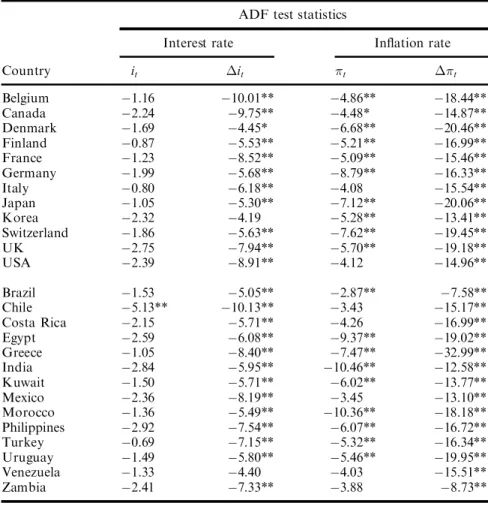
suggests these two variables must be cointegrated. Therefore, ®rst the unit root tests of the interest rate, in¯a-tion and their ®rst di erences are reported in Table 10. The presence of unit roots in interest rates cannot be rejected for any countries except for Chile at the conventional 5% level of signi®cance. However, their presence in in¯ation can be rejected for all the countries except for Italy, the USA, Chile, Costa Rica, Mexico, Venezuela and Zambia. (Engsted, 1995, also ®nds similar results for some of the countries in his sample.) Therefore, the empirical evidence
presented in the table may suggest that there is no long-run relationship between these variables; and the real interest rate may include a unit root. This is not what most of the macroeconomic models suggest even if King et al. (1991) imply that the real interest rate is nonstationar y for the USA within the real business cycles framework. Another reason could be that even if one cannot reject the unit root in interest rates, they are in fact stationary through near-integration.
In order to see if there is a spurious relationship between the interest rates and in¯ation, the Engle and Granger (1987) type of cointegration test was performed. After regressing the interest rate on a constant term and in¯ation. Column I of Table 11 reports the ADF tests statistics of the residuals. One can reject the null of unit root in 17 out of 26 cases at the 5% level of signi®cance. This speci®cation does not account for the short-run dynamics of the interest rates. The unit root of the residuals for Equation 5 is also tested. The ADF tests are reported in column II of Table 11. One can reject the unit root for all the countries in the sample. Hence, there is a long-run relationship between the interest rate and in¯ation, and the results reported in Tables 2 and 3 are not spurious.3
Table 8. Adjusted models for US data USA Period 1974:01 1981:01 1990:01 1981:01 1990:01 1998:05 Constant 0.222 0.429 0.402 (0.775) (0.164) (0.169) ºt 0.777* 0.5734* ¡0.132* (1.377) (0.488) (0.765) ¢it ¡34.477 ¡11.924 ¡46.964 (91.934) (5.225) (31.276) ¢it¡1 20.754 1.203 20.303 (53.653) (1.463) (12.562) ¢it¡2 ¡16.775 ¡2.108 5.986 (44.550) (2.169) (6.600) ¢it¡3 ± 1.208 ± (1.755) ¢it¡4 ± ¡2.914 ± (2.159) ¢it¡5 ± 3.348 ± (2.304) ¢ºt 1.145 0.305 ¡0.009 (3.898) (0.526) (0.614) ¢ºt¡1 1.743 0.103 0.433 (5.249) (0.451) (0.717) ¢ºt¡2 0.767 ¡0.102 0.698 (2.904) (0.337) (0.835) ¢ºt¡3 0.606 ¡0.241 0.087 (2.574) (0.326) (0.461) ¢ºt¡4 ¡2.719 ¡0.801 0.089 (6.626) (0.403) (0.320) £¶0 1.922 0.879 -0.141 £¶1 0.597 ¡0.203 0.442 £¶2 ¡0.975 ¡0.204 0.264 £¶3 ¡0.161 ¡0.139 ¡0.611 £¶4 ¡3.326 ¡0.560 0.003 £¶5 2.719 0.802 ¡0.089 DW 1.95 1.88 2.04 R2 0.94 0.96 0.99
Standard deviations are given in parentheses.
Standard deviations are corrected for heteroscedasticity with White (1980).
* Do not reject the null hypothesis. ¡ ˆ 1 at the 5% signi®cance level.
Table 9. Robustness analysis for US adjusted models United States
Period 1974:01 1981:01 1990:01 1981:01 1990:01 1998:05
Lags Critical Q-statistics
À2values F-values 1 3.84 0.034* 0.359* 0.084* 3 7.81 0.254* 1.054* 4.097* 6 12.6 4.929* 8.206* 6.633* 9 16.9 8.785* 12.458* 13.755* 12 21.0 10.761* 13.909* 13.970* 15 25.0 16.803* 19.438* 20.566* 18 28.9 18.221* 20.897* 22.405* ARCH-LM test F-values 1 3.84 45.693 5.908 0.0008 3 7.81 18.704 12.451 1.3418 6 12.6 9.1698 23.312 2.138 9 16.9 6.3698 14.882 1.3888 12 21.0 5.1558 7.3928 1.4948 15 25.0 3.9478 5.4698 1.1658 18 28.9 3.4948 5.7878 0.9988
* Does not reject that all of the autocorrelations are zero at the 5% signi®cance level.
8 Does not reject that there is no ARCH at the 5% signi®cance level.
3An alternative to Wickens and Breush’s (1988) method could be Pesaran and Shin’s (1999) cointegration implication of the Autore-gressive Distributed Lag modelling. However, the latter model requires both the interest rate and in¯ation to be I(1). Since Table 10 suggests that in¯ation is I(0), the Pesaran and Shin (1999) approach has been avoided in this study.
I V . C O N C L U S I O N
There is a long tradition of testing the Fisher hypothesis in economics literature. In this study, the available literature have been extended by examining the Fisher hypothesis for a sample of 26 countries using a method that allows one to observe the long-run relationship between interest rates and in¯ation by abstracting from the short-run dynamics of interest rates. In this work, attention was focused on testing the strong version of the Fisher hypothesis: Does the nominal interest rate rise point-for-poin t with the expected in¯ation?
This study ®nds supporting evidence for the strong version of the Fisher hypothesis in 16 out of 26 countries. It is also likely that the Fisher hypothesis holds more for the developed countries than the developing ones in the sample. The strong version of the Fisher hypothesis could not be rejected for 9 out of 12 developed countries and for 7 out of 14 developing countries.
A C K N O W L E D G E M E N T S
The authors wish to thank Anita Akkas° and Mehmet Caner for their helpful comments.
Table 10. Stationarity test for the interest rate and the in¯ation rate ADF test statistics
Interest rate In¯ation rate
Country it ¢it ºt ¢ºt Belgium ¡1.16 ¡10.01** ¡4.86** ¡18.44** Canada ¡2.24 ¡9.75** ¡4.48* ¡14.87** Denmark ¡1.69 ¡4.45* ¡6.68** ¡20.46** Finland ¡0.87 ¡5.53** ¡5.21** ¡16.99** France ¡1.23 ¡8.52** ¡5.09** ¡15.46** Germany ¡1.99 ¡5.68** ¡8.79** ¡16.33** Italy ¡0.80 ¡6.18** ¡4.08 ¡15.54** Japan ¡1.05 ¡5.30** ¡7.12** ¡20.06** Korea ¡2.32 ¡4.19 ¡5.28** ¡13.41** Switzerland ¡1.86 ¡5.63** ¡7.62** ¡19.45** UK ¡2.75 ¡7.94** ¡5.70** ¡19.18** USA ¡2.39 ¡8.91** ¡4.12 ¡14.96** Brazil ¡1.53 ¡5.05** ¡2.87** ¡7.58** Chile ¡5.13** ¡10.13** ¡3.43 ¡15.17** Costa Rica ¡2.15 ¡5.71** ¡4.26 ¡16.99** Egypt ¡2.59 ¡6.08** ¡9.37** ¡19.02** Greece ¡1.05 ¡8.40** ¡7.47** ¡32.99** India ¡2.84 ¡5.95** ¡10.46** ¡12.58** Kuwait ¡1.50 ¡5.71** ¡6.02** ¡13.77** Mexico ¡2.36 ¡8.19** ¡3.45 ¡13.10** Morocco ¡1.36 ¡5.49** ¡10.36** ¡18.18** Philippines ¡2.92 ¡7.54** ¡6.07** ¡16.72** Turkey ¡0.69 ¡7.15** ¡5.32** ¡16.34** Uruguay ¡1.49 ¡5.80** ¡5.46** ¡19.95** Venezuela ¡1.33 ¡4.40 ¡4.03 ¡15.51** Zambia ¡2.41 ¡7.33** ¡3.88 ¡8.73**
The critical values are ¡5.24, ¡4.70, and ¡4.42 for a sample size of 480, at the 1% , 5% , and 10% signi®cance levels, respectively (MacKinnon, 1991). A constant and 4 lags are included in the test regression.
** Reject the null hypothesis of the unit root at the 5% signi®cance level. * Reject the null hypothesis of the unit root at the 10% signi®cance level.
R E F E R E N C ES
Bewley, R. A. (1979) The direct estimation of the equilibrium response in a linear dynamic model, Economic Letters, 3(4), 357±61.
Boudoukh, J. and Richardson M. (1993) Stock returns and in¯a-tion: a long-horizon perspective, American Economic Review, 83, 1346±55.
Carmichael, J. and Stebbing P. W. (1983) Fisher’s Paradox and the theory of interest, American Economic Review, 73(4), 619±30.
Crowder, W. and Wodar, M. E. (1999) Are tax e ects important in the long-run Fisher relationship? Evidence from the muni-cipal bond market, The Journal of Finance, 54(1), 307±17.
Darby, M. (1975) The ®nancial and tax e ects of monetary policy on interest rates, Economic Inquiry, 13, 266±76.
Engle, R. F. (1982) Autoregressive conditional heteroscedasticity with estimates of the variance of United Kingdom in¯ation,
Econometrica, 50, 987±1007.
Engle, R. F. and Granger, C. W. J. (1987) Cointegration and error-correction: representation, estimation, and testing.
Econometrica, 55, 251±76.
Engsted, T. (1995) Does the long-term interest rate predict future in¯ation? A multi-country analysis. The Review of Economics
and Statistics, 77, 42±54.
Gordon, R. J. (1971) In¯ation in recession and recovery.
Brookings Papers, Washington, 105±58.
Hsiao, C. (1979) Causality tests in econometrics. Journal of
Economic Dynamics and Control, 1, 321±46.
King, R. G., Plosser, C. I., Stock, J. H. and Watson, M. W. (1991) Stochastic trends and macroeconomic ¯uctuations,
American Economic Review, 81, 819±40.
Koustas, Z. and Sertelis, A. (1999) On the Fisher e ect. Journal of
Monetary Economics, 44, 105±130.
Lahiri, K. (1976) On the constancy of real interest tates. Economic
Letters, 1(3), 45±8.
Lothian, J. (1985) Equilibrium relationships between money and other economic variables, American Economic Review, 75(4), 828±35.
Lucas, R. (1980) Two illustrations of the quantity of money,
American Economic Review, 70(5), 1005±14.
MacKinnon, J. (1987) Critical values for cointegration tests, in R. F. Engle and C. W. J. Granger (eds) Long-Run Economic
Relationships, Cambridge University Press, Cambridge.
Mishkin, F. S. (1992) Is the Fisher e ect for real? A re-examin-ation of the relre-examin-ationship between in¯re-examin-ation and interest rates.
Journal of Monetary Economics, 30, 195±215.
Moazzami, B. (1989) Interest rates and in¯ationary expectations: long-run equilibrium and short-run adjustment, Journal of
Banking and Finance, 14, 1163±70.
Moazzami, B. and Gupta, K. (1995) The quantity theory of money and its long-run implications, Journal of Macroeconomics, 17(4), 667±82.
Pesaran, M. H. and Shin, Y. (1999) Autoregressive distributed lag modelling approach to cointegration analysis, in
Econometrics and Economic Theory in the 20th Century
Strom (ed.), Cambridge University Press, Cambridge. Rossana, R. and Seater, J. (1995) Temporal aggregation and
eco-nomic time series, Journal of Business and Ecoeco-nomic
Statistics, 13(4), 441±51.
Tanzi, V. (1980) In¯ationary expectations, economic activity, taxes and interest rates, American Economic Review, 70, 12± 21.
Thornton, J. (1996) The adjustment of nominal interest rates in Mexico: a study of the Fisher e ect. Applied Economics
Letters, 3, 255±57.
Tobin, J. (1965) Money and economic growth. Econometrica, 33(4), 671±84.
Wickens, M. R. and Breush, T. S. (1988) Dynamic speci®cation, the long-run and the estimation of transformed regression models. The Economic Journal, 98, 189±205.
White, H. (1980) A heteroskedasticity-consistent covariance matrix and direct test for heteroskedasticity. Econometrica, 48, 817±38.
Yuhn, K. H. (1996) Is the Fisher e ect robust? Further evidence,
Applied Economics Letters, 3, 41±4.
Table 11. Test on the linear telationship
I II
Country Statistic Statistic
Belgium ¡1.70* ¡10.55*** Canada ¡2.69*** ¡9.30*** Denmark ¡1.67* ¡4.76*** Finland ¡0.59 ¡6.91*** France ¡2.21** ¡9.54*** Germany ¡2.18** ¡6.79*** Italy ¡2.16** ¡7.40*** Japan ¡0.07 ¡9.73*** Korea ¡1.66* ¡6.15*** Switzerland ¡2.20** ¡6.00*** UK ¡2.91*** ¡8.94*** USA ¡8.29*** ¡8.29*** Brazil ¡2.49** ¡2.22** Chile ¡1.68* ¡5.95*** Costa Rica ¡5.54*** ¡6.55*** Egypt ¡2.18** ¡6.75*** Greece ¡2.54** ¡10.17*** India ¡1.98** ¡7.04*** Kuwait ¡2.23** ¡6.29*** Mexico ¡1.66* ¡7.51*** Morocco ¡3.30*** ¡5.25*** Philippines ¡1.32 ¡7.38*** Turkey ¡2.32** ¡5.09*** Uruguay ¡2.31** ¡6.38*** Venezuela ¡1.66* ¡4.38*** Zambia ¡2.50** ¡5.06***
The critical values are ¡2.57, ¡1.94, and ¡1.62 at the 1% , 5% , and 10% signi®cance levels, respectively (MacKinnon, 1991). No intercept, no trend and 4 lags are included in the test regression, except for Denmark 2, Greece 2, Turkey 3 and Vene-zuela 2.
*** Reject the null hypothesis of the unit root at 1% signi®cance level.
** Reject the null hypothesis of the unit root at the 5% signi®cance level.
* Reject the null hypothesis of the unit root at the 10% signi®cance level.