' ş Η*'νΎ^Ο·νν^ΐ Sitili* · · ■ ' ·
Ä T5-ES;S
JOINT LOT SIZING AND TOOL MANAGEMENT IN
A SINGLE CNC ENVIRONMENT
A THESIS
SUBMITTED TO THE DEPARTMENT OF INDUSTRIAL ENGINEERING
AND THE INSTITUTE OF ENGINEERING AND SCIENCE OF BILKENT UNIVERSITY
IN PARTIAL FULFILLMENT OF THE REQUIREMENTS FOR THE DEGREE OF
MASTER OF SCIENCE
By
din
October, 1996
*1 91ra cedd t A 0 oeASiraceddiu ONEN
ь
é S
•OS4
1ЭЗб
II
1 certif.y that I luive read this thesis and that in iny opinion it is i'nily adequate, in scope and in qucility, as a thesis for the degree of Master of Science.
O (I r
Assist. Prof. M. Sefirn Aktiirk (Advisor)
I certify thcit I hcwe reci.d this thesis and that in iny opinion it is fully ade((uate, in scope and in quality, as a thesis for the degree of Master of Science.
Assoc. Prof. Siimn Kayahgil
I certily that I have read this thesis and that in iny opinion it is fully adequate, in scope and in qucdity, as a thesis for the degree of Master of Science.
Assoc. Prof. Ihsan Sabuncuoğlu
Approved for the Institute of Engineering and Sciences:
Prof. Meninet liaTciy
ABSTRACT
JOINT LOT SIZING AND TOOL MANAGEMENT IN A
SINGLE CNC ENVIRONMENT
Siraceddin ÖNEN
M.S. in Industrial Engineering
Sui)ervisor: Assist. Prof. M. Selirn Aktiirk
October, 1996
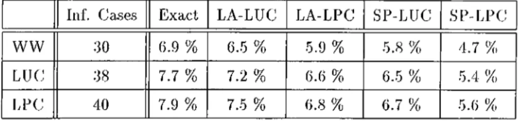
111 most of the studies on tool management, lot sizes are taken as pi'edetermined input while deciding on tool allocations and machining |)arameters. In this study, we considered the integration of lot sizing and tool rnaricigement problems for single and multi i:>eriod cases. For the single period case, we proposed a new algorithm. By this algorithm we not only improved the overall solution by exploiting interactions, but also prevented any infeasibility that might occur lor the tool management problem due to the decisions made at the lot sizing level. The computational experiments showed that in a set of randomly generated problems 22.5% of solutions found by a. traditional approach were infeasible and the proposed joint approach improved the overall solution by 6.8%. For the multi period case, we proposed live new algorithms. Among these algorithms, the most promising one was tlie Look Atiea.d-LUC algorithm, which improved the overall solution on the average by 6.5% compared to the best known algorithm, Wa.gner-Whitin, used in traditional approcich, over a set of randomly generated problems.
Key -words: Flexible Manufacturing Systems, Lot Sizing, Tool Management
ÖZET
BİLGİSAYAR KONTROLLÜ İMALAT SİSTEMLERİNDE
KAFİLE BÜYÜKLÜĞÜ VE KESİCİ UÇ İŞLETİMİ
PROBLEMLERİNİN ENİYİLEMESİ
Siracecldin ÖNEN
Endüstri Mühendisliği Bölümü Yüksek Lisans
Tez Yöneticisi: Yard. Doç. Dr. M. Selim Aktürk
Ekim, 1996
Kesici uç işletimi ile ilgili yapılmış pek çok çalışmada, kesici uç dağılımı ve üretim şartları belirlenirken kafile büyüklükleri önceden belirlenmiş sabit
değerler olarak alınmışlardır. Bu çalışmada tek veya çok dönem üretim
durumlcirında kafile büyüklüğü ve kesici uç işletimi problemlerinin birada ('iıiyilcnmesi amaçlanmıştır. Tek dönem modelinin çözümü için önerdiğimiz yeni metodu farklı şartlar gözönünde bulundurularak üretilen bir küme
problem üzerinde test ettik. Bu metot ile klasik yaklaşımda %22.5 olan
olursuzluğu önlemekle kalmayıp, ortalama %6.8 lik l)ir maliyet indirimi
gerçekleştirdik. Çok dönem modelinin çözümü için ise beş farklı çözüm
metodu önerdik. Önerdiğimiz çözüm metotlarını farklı şartlar gözönünde
Inılundurularak üretilmiş bir küme problem üzerinde test ettik. Önerdiğimiz çözüm metotları çırasında özellikle İkincisi çözüm süresi ve ortalama maliyet indirimi gibi performans ölçütleri dikkate alındığında en iyi metot olarak göze çarpmaktadır. Bu metot ile klasik yaklaşımda en iyi sonucu veren Wagner- VVlıitin metoduna kıyasla %6.5’lik bir maliyet indirimi gerçekleştirdik.
Anahtar sözcükler: Esnek Üretim Sistemleri, Kafile Büyüklüğü Belirlen
mesi, Kesici Uç işletimi
ACKNOWLEDGEMENT
I a.m indebted to Assist. Prof. Selirn Aktiirk for his invaluable guidance, (u icon rage merit and above all, for the enthusiasm which he inspired on me during this study.
I am also indebted to Assoc. Prof. Ihsan Sabuncuoğlu and Assoc. Prof. Sinan Kayahgil for showing keen interest to the subject m atter and accepting 1.0 read and review this thesis.
1 would also like to thank to rny classmates Bayram Yddirirn , Murat Aksu,
Ki'dein Eskigün and my hornernates Abdullah Daşcı and Kemal Kılıç tor their friendship and patience.
f'diially, I would like to thank to rny parents and everybody who has in some wa.y contributed to this study by lending moral support.
C o n ten ts
1 Introduction
2 Literature R eview
3 Problem Statem ent 13
3.1 Problem Definition and Assumptions
3.2 Lot Sizing Decision
3.2.1 Economic Order Quantity (EOQ) Model 17
3.2.2 Wagner-Whitin (WW) Model
3.2.3 Least Unit Cost (LUC) Model... 18
3.2.4 Least Period Cost (LPC) Model
3..3 'I'ool Management Decisions 19
3.3.1 Notation 20
3.3.2 Mcitliernatical M o d e l... 21
3.3.3 Single Machining Operation Problem (SMOP) . . . . 24
3.3.4 Exact Solution Procedure 2.5
3.4 Summary 28
4 Single Period M odel 29
4.1 Problem Definition and Notation ;}()
4.2 Mathemcitical M o d e l... 32
4.3 A lg o rith m ... 35
4.4 Numerical E x a m p le ... 4()
4.5 Computational R e s u lts ... 44
4.6 Summary 49 5 M ulti Period M odel 51 5.1 Problem Definition and Noted,ion 52 5.2 Mathematical M o d e l... Fyi-5.3 Algorithms... ,56
5.3.1 Exact Algorithm ,58 5.3.2 Look Ahead-LUC (LA-LUC) A lg o rith m ... 60
5.3.3 Look Ahead-LPC (LA-LPC) A lg o rith m ... 61
5.3.4 Single Pass-LUC (SP-LUC) A lgorithm ... 61
5.3.5 Single Pass-LPC (SP-LPC) A lg o rith m ... 62
5.4 Numerical E x a m i^ le ... 63
5.5 Computational R e s u lts ... 67
5.6 Summary 73
CONTENTS IX
6 Conclusion 74
G.l C o n trib u tio n s... 74
G.2 Future Research Directions 7G
B IB L IO G R A PH Y 77
A TABLES of the SINGLE PER IO D MODEL 82
B TABLES of th e MULTI PERIO D MODEL 86
L ist o f F igu res
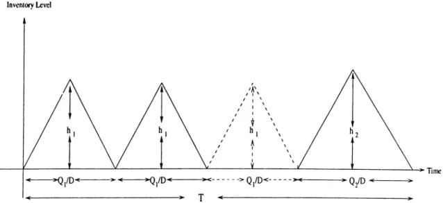
4.1 Inventory Level versus Time...
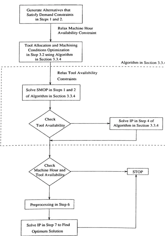
1.2 Flow Chart of the Algorithm 36
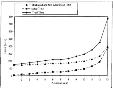
4..3 The Detailed Analysis of Cost Components for Pa.rt 2 The Detailed Analysis of Time Components for Part 2
L ist o f T ables
4.1 Alternative Production S ch ed u les... 41 4.2 Optimum Tool Allocations for the Eqiud Lots of PcU't 1 ... 42
4.3 Optimum Tool Allocations for the Last Lot of Part 1 44
4.4 Optimum Tool Allocations for Part 2 ... 44 4.5 ExperiiTientcd F a c to rs... 45 4.6 Overall Results of the Experimental Design... 48 4.7 Percent Improvements and the Number of Infeasible Oases . . . 48
4.8 F' Values and Significance Levels (p) for ANOVA Results . . . . 48
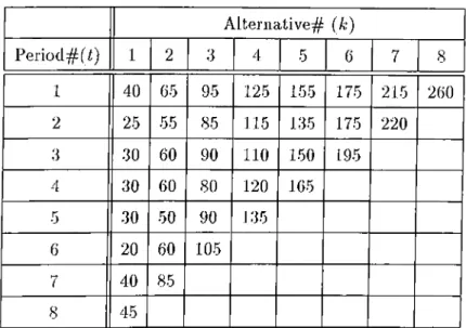
5.1 Alternative Lot Sizes {Qptk) foi’ Paid, 1 64
5.2 Total Cost (Cpik) Values for Lot Sizes of Part 1 64
5.3 Proposed Lot Sizes and Total Cost Values for Part 3 66
5.4 Total Cost Vcilues and Percent Improvements 67
5.5 Experimental F a c to rs... 68
5.6 Number of Infeasible Cases and Percent Improvements 70
5.7 Computation Time (sec.) Results lor the Algorithms 70
LIST OF TABLES X ll
5.8 F Vcilues cind Significance Levels (p) for ANOVA Results . . . . 71 5.9 Percent Improvements and the Number of Infeasible Cases . . . 72
A.I Tooling Information 82
A.2 Possible Operation-Tool Assignments for P a r t s ... 83 A.3 Data for Numerical E xam ple... 83
A.4 Operation Data for Pcvrt 1 84
A.5 Opei’cition Data for Part 2 ... 8'1 y\.6 Actual Tool Reciuirements for Alternatives of Part 1
A.7 Actual Tool Requirements for Alterricitives of Part 2
84 85
A.8 Teclmologiccd Exponents and Coefficients of the Available Tools 85
B.i Cost and Time Data Related to Parts 87
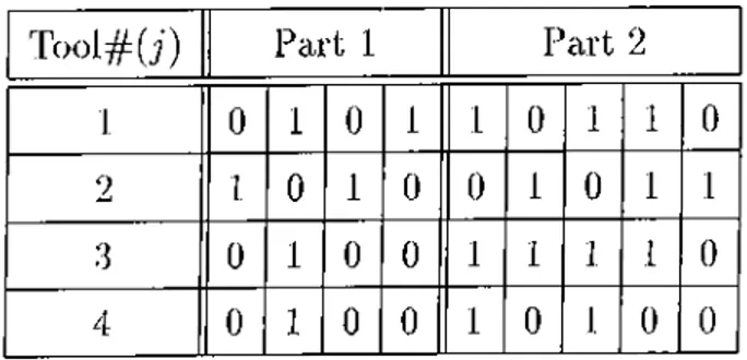
0.2 Opercition-Tool Assignments and Operation Data for Parts . . . 88 0.3 Tool Availabili
0.4 'Fooling Information
0.5 Toted Mcichine Hour (Tptk) Requirements for Lot Sizes of Paii 0.6 Lot Sizes Pi'oposed by the Excict Algorithm
0.7 Lot Sizes Proposed by the Look Ahead-LUC Algorithm 0.8 Lot Sizes Proposed by the Look Ahecvd-LPC Algorithm 0.9 Lot Sizes Proposed by the Single Pciss-LUC Algorithm O.IO Lot Sizes Proposed by the Single Pass-LPC Algorithm
89 89 90 90 91 91 92 92
LIST OF TABLES X I11
B .ll Lot Sizes Proposed by the Wcigner-WIiitin (WW) Algorithm . . 93
B.12 Lot Sizes Proposed by the Lecist Unit Cost (LUC) Algorithm 93
C h a p ter 1
In tro d u ctio n
Many cornpcuiies have recUized that in order to compete in today’s world market, they must rely on innovcitive developments in manuiacturing tech nology. 'lb increase productivity, companies are applying computer controlled machine tools, automated materials handling and storage systems. Due to the progress in manufacturing technology and organization, the concept of flexible manulacturing systems (FMSs) luis emerged. FMSs can be defined as computer controlled production systems capable of processing a variety of part ty|)(;s. d’he main components of such a system are.
• Computer numerically controlled (CNC) machines including the tools to operate these machines,
• An automated material handling system (MHS) to move the workpieces through the system, and
• On line computer control to manage the entire FMS, including CNC ma.chines and the
'These systems may differ enormously in the extent of automation and tlie diversity of the parts. An FMS is designed to achieve the efliciency of botli automated high volume mass production and flexibility of low volume job shop
CHAPTER 1. INTRODUCTION
production. Due to the complex nature of FMSs, the related production management problems are also more complex than other manufacturing s,ystems. Therefore, the efficient operation of an FMS is a very difficult task, and in many implementations the available capacity is underutilized. In view of tin; high initial cost of the FMSs, it is important to operate these systems (dficiently as much as possible in order to get expected benefits of fh'xibility and economy.
In FMSs tool related issues are the key factors for the overall system |)erlbrniance due to their impact on Iroth cost figures and tlie operational c.onsidera.tions. The cutting tool utilization is important for the entire system performance especially in metal cutting industries due to the high metal removal rate in metal cutting processes, and the consequent increased tool consumption rates and tool replacement frequencies.
In manufacturing industry, due to the complexity of the planning proljhvrn, materials requirement planning (MRP) based systems are extensively used
for managing production. In such environments, the lot sizing and tool
management problems are solved independently. The lot sizing problem is considered as a. planning problem and is assumed to be solved at a higher level in an organization than is the tool management problem, whereas the tool management problem is considered a low level detailed decision prol:)lem tliat should be solved after the lot sizing problem. Consequently, these two problems aix! solved independently in a two-level approach ignoring tlie interactions such as production rates, tooling costs, tool and machine hour capacity constraints, between these two levels. However, in a two-level approach determining lot sizes prior to the tool management decisions may result in either suboptimaJ or inleasible solutions.
In this study, we will consider the integration of lot sizing and tool management problems on a single CNC turning machine and discuss the joint problem for both single and multi period cases. After giving the mathematical formulation of the problem, we will present some new algorithms to solve this |)roblem lor both of the cases. All of the proposed algorithms will be tested
CHAPTER 1. INTRODUCTION
on a. set of randomly generated problems, and step-by-step execution of tire algorithms will be given on numerical examples.
'I'lie remainder of the thesis can be outlined as follows. In the next
( liapter, we will give a short review of the literature on the lot sizing and tool management problems including existing few studies on the integration of tlii'se two problems. In Chapter 3, we will give the definition of the problem and tire underlying assumptions in addition to the notation used throughout tlie thesis. In this chapter, we will concentrate on independent lot sizing and tool inanagement problems. In Chapters 4 and 5, the joint problem will Ire studied for single and multi period cases, respectivcrly. In these chapters, we will give tli(' mathematical models as well as the algorithms and the computational li'sults of the experimental designs. Finally, in Chapter 6, some concluding r(imarks and suggestions for future research are provided.
C h a p ter 2
L itera tu re R ev iew
l*'Iexil)le iTicUiufacturing systems (FMSs) typically contain a set oi numerically coiitrollecl workstations and a material liandling system coordinated by a centra] controller for the purpose of simultaneous production of a variety of part types. The FMS represents a significcuit investment in training, Imrdvvare a.nd
software. This investment is justified the ability of the system to produce
a. variety of high quality parts with short lead times while requiring less floor· s|)ace than traditional systems [33]. An FMS Ims the cdDility to pi’oduce a family ()(' pa,i ts in a flexible way. To realize these potential benefits, cai'eful attention must be paid not only to design but cilso to planning of the system once it has iK^en installed. Since FMSs are usually a part of a multistage manufacturing system, inputs and outputs are dictated by the master production plan, 'rhis plan specifies availability dates tor raw materials and components, arid due dates for finished products. The FMS production planning problem consists of organizing production such as to satisfy the master production plan as well as to obtain an efficient use of system resources (machines, pallets, fixtm-('s,
tools etc.). In an FMS of reasonable size, this planning process is (|uite
com|)lex. Agciin, it is helpful to decompose the problem into ci set of smaller and manageable subproblems [2].
There are critical tool management issues that affect the productivity
CHAPTER 2. LITERATURE REVIEW
aiicl machine tool supiDliers recognize that a lack of attention to such tool umnagernent issues is a primary reason for the j^oor iDerformance of many facilities. Grciy et ciL [17] classify tool mcinagernent issues into tool-level, ma.chine-level and system-level issues. The “tools” they are concerned with are the cutting or shaping tools residing in an automated computer numerical control (CNC) “nmchine” used to remove metal from castings. A “system” is an integrated production facility with several automated machines and, perliaps, automated handling of parts cirid tools. The classification of tool, nmchine and system level issues allows one to portray how individual tool-rela.ted models may fit into machine level models and how technological constraints diixictly aifect key operational decisions at all levels.
In the literature it is stated that approximately 50% of U.S. annual expenditures on manufacturing is in the metid-working industry, and two- tliirds of metal-working is inetcil cutting. In ciddition 75% of the dollar volume of metal worked products is manufactured in batches of less than 50 parts [54]. Besides being a critical issue in fcictory integrcition, tool management has direct cost implications. Veerarnani et al. [44] emphasized that the lack of tooling considerations has resulted in the poor performcmce of automated manufcicturing systems. Kouvelis [25] identified cutting tool utilization as an important parameter for the overall system performance. In this study, the cost of tooling has been reported to l)e 25-30% of the fixed and variable cost of production. Manufacturing management publications have recently |)aid considerable attention to the benefits of improving the integration of tool management within total system design, planning, scheduling and control [17].
Most of the existing studies in the literature on tool management ignore' the lot sizing decision at system level and tcike it cis a predetermined input while deciding on tool allocations and rricichining pcirameters. Cray et al. [17] |)ointed out that, efforts in tool management locus on single level decisions, altliough a decision nuicle at a higher level without considering its impact on Idle lower levels can lead to either infeasible or inferior results. Lot sizing is such a decision which is taken at system level ignoring its impact on lower
CHAPTER 2. LITERATURE REVIEW
('xisting studies on tool mcmcigement, lot sizes a.re taken as precletennined
input while deciding on tool allocations and machining parameters. In
an automated manufacturing environment operational [)roblems such as ma,chining conditions, tool civaikibility and tool life should be taken into account for the reliable modeling of CNCs, or the absence of such crucial
constraints may lead to infecisible results. It has been shown in sevcM'al
studies that significant cost savings can be realized by controlling production rates (Cheng et al. [7], .Jones and Inrncin [21], Silver [31], Strusevich [35]). Consequently, total production cost can be decreased and any inlV;asibility due to ma.chine hour capacity limitation can be cwoided.
For solving the tool allocation problem at the system level, most of the published studies use 0-1 binary variables, i.e. a particular tool j is assigned to operation i, to represent tool requirements. Stecke [34] Ibrmulates the FMS loading problem as a nonlinear iriixed integer progrcuriming (MIP) problem and solves it through linearization techniciues. Sodhi et al. [33] propose a four level hierarchy lor production control of FMSs, including part type selection and loading, and present various models at ecich level. Sa.rin and Chen [30] give an K4IP formulation under the assumption that the total machining costs de|)end upon the tool-machine combination. The tool life is considered as a. constra.int ii) tlie formulation. Unfortunately, all of these studies assume constant lot sizes, production rates as well as processing times. Furthermore, these studies determine the tool requirements lor each operation independently, and fail to relate the contention among the operations for a limited number of tools.
At the machine level, there exist several studies paying attention to tooling issues like tool selection, tool magazine loading and minimized,ion of tool switches due to a change in a part mix, at both the long term planning and o|)erational level (Bard and Feo [4], Crcuria et cil. [8], Kouvelis [25], Tang and Denardo [37]). Unfortunately, these studies also assume constant lot sizes, processing times and tool lives, even though the tool replacement frequency is directly rekrted with the machining conditions selections. Further, in the multiple operation case, non-machining time components, such as tlie tool rephicernents due to tool wear, can have a significant impact on the total cost
oC production and the throughput of parts as shown by Tet/dafF [38]. Gray et aJ. [17] reported that tools are chcinged ten times more often due to tool wear than to part mix because of the relatively short tool lives of many turning tools.
CIIAPrER 2. LITERATURE REVIEW 7
The machining conditions optimization for a single operation is a well known problem, where the decision variables are the cutting speed and feed rate. Several models and solution methodologies have been developed in the literature (Ermer [11], Gopalakrishnan cuid Al-Khayyal [14], Tan and Greese [36] ). However, these models consider only the contribution of machining time and tooling cost to the total cost of operiition, usually ignoring the contribution of non-nicichining time comi^onents to the operating cost, whicli could be very significant for the multiple operation case. Further, these studies exclude the tooling issues such as tool availability and tool life capcicity limitations.
In a recent study, Akturk and Avci [1] proposed a new solution procedure to make tool allocation and machining conditions selection decisions simultaneously by considering the related tooling considerations of tool wear, tool availability, and tool reiDlacing and loading times, since they affect both I,he machining and non-machining time components, hence the total cos!, of |)roduction. In this study they extended single machining operation probhuri (ShdOP) formulation by adding a new tool life constraint, which enabled them to include tooling issues like tool wear and tool availability. Furthermore, they proposed a new cost measure to exploit the interaction between the iiundrer of tools required with the machining, tool replacing and loading times, and l.ool wa.ste cost in conjunction with the optimum machining conditions for alternative operation-tool pairs. Consequently, they prevented any infeasibility l.liat might occur for the tool allocation prol^lem at the system level due to tool contention among tool life restrictions through a feedback mechanism.
'The importance of effective lot sizing is well recognized by both pra.cti- tioners and researchers, and the lot sizing problem, in a variety of forms, lias received much attention in the literature. Lot sizing problems pla.y an important role in modern production planning systems, such a.s materials
CHAPTER 2. LITERATURE REVIEW
r('quirernent planning (MRP), hierarchical production planning (ИРР) and just in time (JIT) manufacturing. Therefore research to develop and improve solution procedures for lot sizing problems is of eminent importance. Although many interesting real life problems in lot sizing remelin unsolved, a still growing number of them can be solved successfully as stated by Salomon [29] in his I^li.D. thesis in which he studied гпешу deterministic lot sizing modiJs.
For relatively simple manufacturing environments, under the assumption that there is a single product and an infinite production capacity, efficient
solution procedures have been developed in the literature. The famous
('cononiic order quantity (EOQ) model was developed by Harris [19] in 1913. 'I'liis model assumes a simple single product, single machine situation with instantaneous replenishments in which d(;mand is stable and inventoiy holding costs and machine setup costs are deterministic and constant over time. After introduction of the EOQ model, Wcigner and Whitin [45] developed an e.xtension of this model in 1958, in which time phased dynamic demand over a finite planning horizon was considered. Nonetheless, when the manufacturing process is more complicated, as will often be the case in practice, problem complexity may increase formidably. Some of complicating factors in the manufacturing process are,
• Dynamic demand
• Nonlinear cost structure • Capacity restrictions • Setup times
In the late fifties Manne [28], and in the sixties and seventies Lasdon and 'lerjung [26] and Zangwill [47] among others started working on lot sizing models for more complex mcinufacturing situations, in wliicli multiph' |)i'oducts, capacity restrictions and machine setup times play an important
rokx Besides the more theoretical work on lot sizing models, a large
CHAPTER. 2. LITERATURE REVIEW
'I'he considercible number of publications in international specialist journals reporting on successful lot sizing applications in industry, e.g. Cunther [18], Van Nunen and Wessels [42], Van Wassenhove and De Bodt [43], demonstra.tes tliat research on lot sizing models is not only of theoretical interest, but also of large practiced value.
In the uncapacitated dyiicimic lot sizing problem, the objective is to minimize the total of fixed costs and holding costs. In each period / of a 'I'-period horizon, lot size (Qt) vedues are to be determined for a. given demand
{(It), 'rids choice also determines the inventory quantity (//,) at the end of period
/,. In the process of developing a dynamic programming procedure for finding tlie optimal solution to this problem, assuming nonnegative inventory position and consequently disallowing backlogging, Wagner and Whitin [45] showed that there exists an optiirud solution such that L-i.Qt = 0 lor every /,. 'J'his means l.hat ea.ch order quantity covers demand for an integral numl^er of periods, a. characteristic sometimes Ccdled the Integrality Property. For such dynandc lot sizing problems some heuristic procedures, that retain the integrality property, such as least unit cost (LUC), Silver-Meal or least period cost (IjPC), |)art [KMviod balancing and marginal cost difference heuristics are developed as summarized by Baker [3]. Gorham [16] states that the most commonly used luniristic was the LUC procedure. Under LUC, the various alternative lot sizing decisions lor the first period, Qi, are evaluated according to their cost p('r unit of demand, C{t)jDi, where Dt denotes the cumulative demand of /, periods and C{t) denotes the corresponding total cost. 'Lhe stopping rule calls for setting Q\ = Dt when this ratio first reaches a. local minimum, that is, when C(t)/Dt < C(t 4- l)/Z)/+i. Silver and Meal [32] proposed 'a stopping rule sometimes called the least period cost (LPC) procedure. Their approach is similar to LUC, but the basis lor stopping rule is cost per period rather than cost per unit. Under LPC, the various alternatives for Q\ arc'
evaluated according to their cost per period, The stopping rule calls
for setting Qi = Dt when this ratio first reaches a local minimum, that is, when C( l ) f t < C{t \.)/(t + i).
CHAPTER 2. LITERATURE REVIEW 10
a.iKl Bitran ¿md Yanasse [5] have shown that the single item capacitat(id lot sizing problem (CLSP) is NP-hard even in mciny special cases. Multi item CLSP is also NP-hard except for a few speeded cases (e.g. when all setup costs are zero) as stated in [29]. However, some polynonnal edgorithms exist for some special Ccipcicitated problems. Florian and Klein [12] developed an ()(T ’) dynandc programndng based shortest path algorithm lor a model with concave costs and constant capacities. Love [27] provided an 0 ( 7 '‘) algorithm that searched the extreme points of the solution space for a model with pi('.c(n^'ise linear concave cost functions cuid bounds on inventories. In a record, study, Van lloesel and Wagelmans [41] developed an algorithm that solves the constaid capacity economic lot sizing problem with concave production costs and linear holding costs in 0(T'^) time. This algorithm is based on the standard dynamic programming approach which requires the computation of the minimal costs lor all possible subplans of the production plan. Instead of computing these costs in a straightforward manner, they used structural properties of the optimal sulrplans to arrive at a more efficient implementation. Due to the complexity of more general CLSPs, most of the literature on this problem focus on heuristic sol ution procedures.
The heuristic approaches reported in the literature are classified by Kii'ca. and Kokten [22] into two groups as mathematical programming and common s('nse approaches. The heuristics suggested Iry Thizy and Van VVassenhove [29], Trigeiro [40] and Cattrysse et al. [6] belong to the first class. The first two heuristics are Lcrgrangian relaxation based procedures, ff'he procedures suggested in Cattrysse et al. [6] use the set partitioning formulation of Maime [28] and generate candidcite plans lor the items by several well known heuristics. 'I'he feasible schedules are obtciined by rounding off the LP-relaxation of the s(4, pai-titioning problem. Most common sense heuristics use of a period-by-period approach, in which CLSP is solved on a period by period basis. In each period, lot sizes for all items cU’e determined on the basis of a cost savings criterion. In a. given period, future demand of items are scheduled to be produced in tliat period until no further cost scivings are possible or until all the capacity at that iK'iiod is exhausted. Some of the heuristics reported in the literature which
CHAPTER 2. LITERATURE REVIEW II
use this approach are the ones due to Dixon cind Silver [9], Dogranicici et ah [10], and Gunther [18]. An alternative itein-liy-itein approach for generating solutions to CLSP is proposed by Kirca and Kokten [22]. in this approacli, solutions are generated itei’citively. In each iteration, a set of items among tlie items not scheduled is selected and production schedules over the planning liori/jon lor this set of items are determined.
In a machining environment especially due to the tool and machine lioiir capacity limitations unit production costs as well as unit resource consumption I'ates cannot be determined uidess tool cillocation and machining conditions optimization problems are solved for each possible lot size value, which could l)e a very difficult task due to the computational burden. Also existence of tliese constrcrints cause production cost function to be convex. However, in most of the models developed in the literature unit production costs cuid unit ı■(^source consumption rates cire assumed to be fixed and apriori known, whereas these are decision variables in a machining environment. Furthermore, in most of these studies the production cost function is assumed to be either concave or linea.r due to the economies of scale. Consequently, existence of such prol)lems ma.kes the applicability of ¿ivailable lot sizing procedures almost impossil)le Idr ma.cliining environments.
In the literature there exist few studies on the integration of lot sizing and tool management problems. Wysk et al. [46] introduce lot size considerations in determining the optirncil cutting speed in a single item, single machine, single peiiod problem. Koulamas [2.3] presents a queueing model lor determining auciJytica.lly the optimal lot size in a machining economics prol)lem uruhu·
stocliastic tool life considerations. Koulamas [24] proposes an iterative
procedure for the sirnultiuieous determination of the cutting speed and lot siz(' va.lues in machining systems for single and multiple part cases using the Ijagrangian technique, while the feed rate is taken as a constant. In this study, |)arts are assumed to be composed of single operation. Consequently, parts ai'e machined by a single cutting tool and tool allocation decisions a.re not considered. The a.uthor also has not considered machine liorsepower, surfa.c(' iinish and tool availability constraints, although in many real life problems tlu^
CHAPTER 2. LITERATURE REVIEW 12
inacliining pcirarneters cire constrained by these limitations. Furthermore, in all of’ tliese studies only single period case is considered cuid consequently demand is assumed to be fixed.
'I'he objective of the research reported in this thesis is to show that there is a. close relationship between the lot sizing and tool management decisions l)y proposing some algorithms for single cind multi period cases of the joint |)roblem. In the next chapter, we give the definition and the underlying a.ssumptions of the problem as well as the details of the algorithm proposed l)y Akturk and Avci [1] to solve tool alloccition and machining conditions optimization problems simultcineously. Our joint algorithms for the integration of lot sizing problem to the tool management problem lor single and multi period cases are given in Chapters 4 and 5, respectively. Finally in Chapter 6, some concluding renuirks cind future research suggestions are provided.
C h a p ter 3
P ro b lem S ta tem en t
UiK' to tlie complex nature of flexible manufacturing systems (FMSs), tlie r<'la,t(xl production maiuigernent problems cire also more complex tlian of,her manufacturing sj^stems. Therefore the efficient operation of an FMS is a very dilficult task, and in many im23lementations the avciilable capa.city lias Ireen underutilized. In view of the high initial cost of the FMSs, it is very importa.n1, to opera.te these systems efficiently as much a.s j^ossible in order to get expected bi'iiefits of flexibility and economy.
in Fh/JSs, lot sizing is one of the important issues which needs further consideration. In the traditional approaches, lot sizing decisions arc given at system level, independent of tool management decisions. However all of tliese d('cisions are closely related and lot sizing decisions affect tool allocations a,s well as machining conditions such as cutting speed and feed rate. Furthermorf', the interaction between lot sizing decisions and production rates in addition to the tool cuicl machine hour capacity constraints cannot be ignored. Integration of tliese decisions ca.n result in reductions in the total production cost and |)i event any infeasibility due to the tool and machine hour capacity constraints.
Tlie organization of this chapter is as follows. In §3.1 the definition of the |)roblem and underlying assumi^tions are given. In §3.2 the lot sizing d(icision is summarized along with a description of some well-known uncapacitated
CHAPTER 3. PROBLEM STATEMENT 14
lot, sizing heuristics. In §3.3 the tool management decisions including a
mathematical model and an exact algorithm to solve tool allocation and machining conditions optimization problems simultcuieously are discussed. l·'inally, some concluding remarks are provided in §3.4.
3.1
Problem Definition and Assumptions
111 tills study an automated machining environment consisting oF a single (!NC machine is considered. The limits of the problem are defined by stating o|)erating policy and characteristics of the system. The Ibllowing assumptions are made to define the scope of the study:
• Production may take place in a single period under static demand or in multiple periods under dynamic demand.
• 'I'liere ¿ue multiple parts in demanded quantities and each part is composed of multiple operations.
• Each operation can be performed l)y a set of alternative tool types with limited qucintities on hand.
• Backlogging is not allowed.
• Initial and final inventory levels are assumed to be zero without loss of generality.
• CNC machine Ccin work for a limited number of hours.
• The tool switching is only allowed during the part changing and only a single tool can be changed at a time. This assumption implies tliat tool changing time occurred in a particulcir part loading/unloading event is additive. So tool changing times of different tools can be summed to find the total tool changing time occurred.
CHAPTER 3. PROBLEM STATEMENT 15
• For the machining operations, the cutting speed and the feed ra.te will be tcdcen as the decision variables, cuid the depth of cut is assumed to be given cxs an input. This assumption particularly limits our attention to single pass machining. Therefore, if a material removal requires more than one pass, those should be prespecified as different v()lumes with their depths.
• Ea.ch nicichining operation of a part should be completed by a. singh; tool type throughout the manufacturing of whole lot. 'riierelbre, during the ma.iiufacturing of ci lot, the same oi)eration of ci part is always macliiuc'd l:>y the same tool type.
• After completion of a lot, remaining tool lives can be used for manufacturing of another lot. Therefore the actrud usage of tools are included in the tooling cost and tool iivciilability rehited calculations.
Under these assumptions we want to solve lot sizing, tool allocation ¿nid machining conditions optimization problems simultaneously to determine the Following decision variables:
• Lot sizing decisions: In what quantities each part will be produced. • Tool m anagem ent decisions:
- Tool allocation: How tools will be alloccited to parts in terms of
(pumtitles and allocation scheme.
— M achining conditions selection: What the cutting speed and
feed rate will be for each operation of each part.
'ITaditional approach for the determination of these decision variables consists of a two-level optimizcition procedure. In the first level, lot sizing decision is given using some lot sizing algorithms cUid in the second level, taking tlie lot sizes Ibund in the first level as input, tool management decisions are given. In the next sections these decisions will be explained in more detail.
CHAPrER 3. PROBLEM STATEMENT L()
3.2
Lot Sizing Decision
'i'lie question of “How much to produce ?” is an important problem that a,lmost ('V(u\y manufacturing business must deal tbi’ smooth a.nd efficient running of its operation. The lot sizing decision answers this question by determining the o|)timum amount that should be produced to satisfy the demand. In a inanufacturing environment using a traditional two level approach, lot sizes are determined by minimizing the total inventory related cost which is usually e.xpix^ssed as the sum of setup and inventory holding costs assuming that unit manufacturing cost is fixed and no shortage cost occurs. The setup cost represents the fixed charge incurred when an order to manufacture is placed. Thus, to satisfy the demand for a. given time period, the more frequent manufacturing of smaller quantities will result in higher setup cost during tlie period than if the demand is scitisfied by less frequent mcuiufacturing of larger (|ua.utities. The holding cost, which represents the cost of carrying inventory in stock (e.g. interest on invested capital, storage handling, depreciation a.nd maintenance) nornicilly increases with the level of inventory.
Dilferent lot sizing models have been proposed according to some denumd characteristics. A deterministic demand may be static, in the sense that consumption rate remains constant with time, or dynamic, where demand is known with certainty but varies from one time period to the next. Without capacity considerations, a multiple part lot sizing problem can be solved for ea.ch item independently tor both of the static and dynamic cases. For the static demand case a. simple economic order quantity (EOQ) model and lor dynamic multi period case Wagner-Whitin (WW), Iccist unit cost (LUC) and h'ast period cost (LPC) algorithms are the most widely used ones. A more' detailed discussion on these approaches can be found in [3] and [20]. Now, we will briefly explain these models below.
CHAPTER 3. PROBLEM STATEMENT 17
3.2.1
E con om ic O rder Q u an tity (EO Q ) M od el
'I’liis model is based on the assumption of continuous and stead,y demand rate. It performs well only where actual demand approximates this assum|)tion. In a single period two level approach EOQ model can be used at system level to find the lot sizes. For the EOQ model, the optimal lot size (Q) is given by the Ibllowing expression: Q = I 2 - S - D h · (I - DIP) where, S h D P
p cost per lot.
Inventory holding cost per unit per period. Demand rate per period, and
Production rate per period {P > D).
l''or nonintegral lot size values, the optimiil Q value can be rounded off. However it is difficult to achieve zero final inventory condition in a single period by producing equal lots of size Q. Because the optimum lot size (Q) found may not exactly divide the demand. In this case it is reasonable to apply l.lie following procedure to get rid of this problem. Let r = [/7/QJ, tlien Q* = D — Q ■ V gives the remaining ciuantity to be produced to satisfy the
demand. If Q* > Q /2, then we produce r lots of size Q and a single lot of size
Q'*. Otherwise we produce r — 1 lots of size Q and a single lot of size Q + Q*.
3.2.2 W a g n er-W h itin (W W ) M o d el
'I’liis model can be used in a two level approach at system level to find tlie optimum lot sizes for multi period dynamic demand cases. Under the assumption of concave or linecir production costs, the optimum production
11
(|uantity in any period is one of these values: 0 or ^ Di for n = 'm + f , · · ·, 7'
t=m
where Di and T denote the demand in period t and the planning liorizon, i('S|)ectively. In another words, if production takes place in any period, tlien
CHAPTER. 3. PROBLEM STATEMENT 18
the entering inventory for that period should be zero. Based on this fact forward and backward dynamic programming algorithms have been developed, '['be solution procedure and a more detailed discussion of this model ca.n be found in [20].
3.2.3
Least U n it C ost (L U C ) M o d el
'Fliis model proposes a heuristic procedure based on the assumptions of the VVVV model. This procedure can be used in a two level a.])j)roa,ch to find tlu^ lot sizes at system level for multi period dynamic demand cases. For the first
period a lot size that covers requirements of t periods is Qn = D i + D2-\--- l·Di
li the fi.xed setup cost for this lot is S and its holding cost is Hi =--- + 2.D:i + · · · + (f — l).Di), then its cost per unit produced is L(KJi ~ ,
V 11
'I'liis algorithm begins with LUC\ (corresponding to Qu) and Ccdculates LIJC2·,
LlJCii etc. until LUCk+i > LUCk- Finding this condition, the procedure sets
the size of the first lot to Qik- In other words, the procedure locates the first local minimum of cost per unit. It then fixes the first lot size at this quantity and proceeds to determine the second lot size. This is accornplislied l),y starting over at time A:+ 1 and searching for the lecist unit cost over periods A:+ 1, A:+ 2, ('tc.
3.2.4
Least P erio d C ost (L P C ) M od el
This model proposes a procedure similar to the one given in the previous section. However, in this method the stopping criterion for the local optimum search is cost per period rather than cost per unit. Using the notations of
the previous section, the minimum cost per period is LPC = The LPC
mc'thod uses this quantity to find a local minimum. Tluit is, the stopping rule dictates that the lot should not be extended further if LPCk+\ >
LPCk-Similar algorithms also exist in the literature tluit can be used to determiiK' I,he lot sizes at system level. However these are the most widely used ones and
CllA PTER 3. PROBLEM STATEMENT 19
(\x;peiiirienta.lly it licis been shown that, these procedures give tiie best results on the avercige among avciilable similar procedures as stated by Baker [3].
3.3
Tool Management Decisions
'Fool management problems cire mainly composed of decisions related to tool allocations iuid machining conditions selection. In this section assuming a fixed lot size, we will give a mathernaticcrl model lor the simultaneous solution ol' these two prol:)lems and an exact solution algorithm proposed |jy Akturk and Avci [1] lor the tool rnaiicigement problem with necessary oixplanations will Ibllow.
Advances in cutting tool materials and designs will increase tire cutting speeds at which machining is carried out, consequently reduce the machining time, Irut the initial tooling cost might be higher. Therefore we consider a set of alternative cutting tool types for each niachining operation, since no one cutting tool type is best for all purposes. Moreover, the same tool may Ire used in several machining operations, each one with differeirt rnaeliining conditions.
The machining conditions optimization for a. single operation is a well known problem and several methods have Ireen developed as discussed in
(lliapter 2. However, these methods only consider the contribution of
macluning time and tooling cost to the toted cost of the operation, where the decision variables are the cutting speed, depth of cut and feed rate. However, in our study of multi operation case, non-cutting time components resulting from dilferent sources, like tool tuning, workpiece loading/unloading etc. have also significant contribution to the toted cost of production via operating cost. All tliese time consundng events except the actual cutting operation are called nou- macldning time components. In our models we only consider tool replacing and loa.diug times, since these are the only ones that can be expressed as a functiou of l)otl) the maehining conditions and alternative operation-tool pairs.
CHAPTER 3. PROBLEM STATEMENT 20
3.3.1
N o ta tio n
Tlie following notation is used throughout the thesis, cv,, /У,, 7 / : Speed, feed, depth of cut exponents lor tool j
(·„,,/>, c,e; Specific coefficient and exponents of the machine power constraint
Co : Operating cost of the CNC machine, ($/min)
f r y , //, / : Specific coefficient cind exponents of the surface roughness constraint
Ctj : Cost of tool _y, ($/tool)
(li : Depth of cut for operation г, (in.)
fij : Feed rate for operation i using tool j , (ipr)
(Ji : Diameter of the generated surface for operation /', (in.) HP,nax '■ Maximum available machine power, (hp)
Set of all opercitions
Set of the available tool types
Set of the candidate tool types for the operation i Length of the generated surface for operation г, (in.)
Number of tool type j required tor completion of operation i
Nj : Number of available tools of type j Q : Lot size, (parts)
Number of times that an operation i сгш be performed l)y a tool type i
: Maximum allowable surface roughness for the operation (//in.)
: Taylor’s tool life constant for tool j
: 'fool magazine loading time for a single tool j , (min.)
: Tool replacing time for tool y, (min.)
: Cutting speed for operation i using tool j , (fprn)
: 0-1 binary decision Vciriable which is equal to 1, if tool j is assigned
to operation i
: 0-1 binary indicator which is eqiuil to 1, if tool j is a candidate tool
for operation i / ./ Ji. L: ''Hi 4i:i SFMi T ( - c tlj Ч Vij Vi:i
CHAPTER 3. PROBLEM STATEMENT 21
3.3.2
M a th e m a tica l M od el
As an introduction, we are going to define some possible time components tlmt sliould be included in the objective function of total cost for the manufacturing of a fixed lot of a single pcirt. There exist two distinct categories for the time components, munely machining time (cutting time) and non-rnachining time (non-cutting or idle time).
• M achining tim e (¿m,:j): Time required to complete a ivKital cutting
operation. For example, the cutting time expression for a turning
operation is given in [15] as follows:
Tv.Gj.Li
/.. , = ___ i__LI r)
r
Y ^.Vij. j i j
Similar expressions for a wide Vciriety of machining operations are a,vailal)le in the literature. However, lor the machining econouucs studies the above expression has been preferred to study on since it is a common ex|)ression to all researchers and ecisy to extend to some other opera.tions.
• Taylor’s tool life expression (T,/): The relationship Iretween machining time and tool life can be expressed as a function of the machining conditions by using an extended form of Taylor’s tool life equation as follows:
T - =
J IJ TC,.7 vN f'!*^‘j t ·)
'Hris expression is frequently used in the ma.chining economics litcra.tui'e, especially in the Ccises where there exist more than one machining condition as the controllable variable.
• Usage rate expression (t/q): For the turning operation l)y combining
above two time expressions, the following expression can be derived for the machining time to tool life ratio.
_ Pnij
^ 3 ~ rp
L ij
TT.Ch.Li.ct;^
CHAPTER 3. PROBLEM STATEMENT 0;)
Consequently, (¡ij = \_i/Uij\ and íг¿j = [Q/<7,·,·]. For pra.ctica.1 purposes, r/,:; must l)e selected in order to instruct either the CNC program or the operator 1.0 cha,nge tools after predetermined number of pieces ha.ve Ijeen machined. Before introducing the rmithematical model some remarks on our assumptions about tool usciges will be helpful. As we stated in §3.1, only the used amounts of tools a.rc! considered in cost ccilculations and tool availability related constraints, 'riiercifore we used an actiuil tool usage expression which is equal to Q ■ Uij for
a. lot size Q and corresponding Uij values.
A mathematical Ibrmulation of the tool allocation and machining conditions o|)timization problem can be as lollows:
Minimize Ct„i, Q - C o - [X] j + C o - {i 'l li j - 1) -l-rj +
\iElj€J / \iEl jEJ ,
+ E E ■■'.j ■ 0 ■ V,, ■ e , ¿e/ ie./
Subject to: · Tool Assignment Constraints:
' ^ X i j = 1, for every i € I jeJ
^ 1^(1 - yij)"^ij = 0 ('€/ jeJ
• Tool Availability Constraints :
Y2 · Q ■ loi· every j 6 J
iei
• Tool Life Constraints :
Xij. Uij . (¡ij < 1, for every i E I, j G J
• Machine Power Constraint:
CHy\PTER 3. PROBLEM STATEMENT 23
• Surface Roughness Constraints :
Xij.Cs-v'ij.fij.d\ < SFMi, for every i G I, j G J
• Nonnegativity and Integrality Constraints :
'Oij > 0, fij > 0, for every i e I, j e J
Xij G {0,1} and Uij nonnegative integer for ev(!ry i G /, j G ·/
in the above rnatheniiitical formulation of the problem, the total cost (Ci„i) of manufacturing of a particuhir lot (Q) is expressed as the sum of operating cost due to machining time cind non-rnachiiiing time components, and tooling costs, respectively. There are four sets of decision VcU-iables. The first set of
decision variables, represents the tool allocation decisions. The second set
of decision varicibles, riij, depicts the number of tools of a given type allocated to an operation. F'diially, the third and fourth sets of decision varial)les, u,;., and /,·,, represent the machining conditions selection decisions.
In tin; presented nonlinear MIP formulation, there exist three l.ypes of constraints, ruirnely, operatiomil, tool related and machining operation constraints. The first set of constraints represents the operational constra.ints vvliich ensure that each operation is assigned to a single tool type of its candidate tools set. The tool civailability and tool life constraints arc; the tool related constraints which guarantee that the solution will not exceed the a,vaila.I)le quantity on hand and the available tool life ca.pacity lor any tool type', respectivel.y. Finally, last two set of constraints represent the usual machining operation constraints. The surface roughness presents the quality r('(|uirement on the operation and the machine power constraint provid('s l,o operate machine tool without being subject to any damage, 'f'he complexity of tlie a.l)ove problem was discussed by Akturk and Avci [1], and they sliowed tliat the tool allocation and machining conditions optimization problem is jV'P- com|)lete and presented a solution algorithm to this problem using the classical single machining operation problem, which will be discussed in the ne.xt section, as a, starting point.
CniAPTER 3. PROBLEM STATEMENT 24
3.3.3
Single M achin ing O p eration P ro b lem (S M O P )
In SMOP, the objective Function includes the tooling cost and o|)(M'ating cost due to the machining time, and it is possible to impose the machining o|)era.tion constraints on the problem together with a tool life constraint. The Following standa.rd mathenuitical tbrmulcition of geometric programming (CP) can be written For the SMOP for every possible operation-tool pair:
.Minimize A L j = C i . v O + C2- v [ j ' ^
Subject to: '* < 1
< 1
< 1
1 J ij A 0
(Tool Life Constraint)
(Macliilie Power (Joustni i iit) (Surface Roughness (Constraint)
where. c \ = TT.Gi.Li.Co , 02 = 7T.Gi.L,.dT.Ct, Cl Y‘L T C j 12 ’ TLTC¡ ^ C„,.(T T T . G i . L i . i i ^ .(Jij ,^.,,1 /'1/ _ ' ·■<■ » - 7 7 7 1 --- 5 '■-'s — 7 T 7 c , 4 S F M ,
Denoting the dual variables by Zi, Z2,..,/^5 flie CP-Dual formulation for the above problem can be as follows:
Maximi:ie
Z/\ /J2
Subject to: '/j\ -|- Z2 — 1
—7j\ A {otj — 1)-2/2 T (tty ~ ^ A b./j,\ A (j-Ar, = 0
- Z i -b ( 4 - l ) . Z2 A ( 4 - l ) . Z - , A C . Z , A k . Z , = 0 Z i , Z 2 . Z : i , Z , , Z , > 0
'I'lie objective for the dual problem is still non-linear, but the constraints of the dual formulation are well-defined linear equations. The dual problem can be
CHAPTER 3. PROBLEM STATEMENT ■>A
solvcxl l)y using the complementary slackness conditions l)etw(ien dual variaJjles and primal constraints, which are given below, in addition to constraints of l)oth the primal and dual problems.
- 1) = 0 - 1) = 0
z u c : . v L f l ^ - 1) = 0
Each of the constraints of the primal problem can be either loose or tight at optimality. If a dual fecisible solution is found lor a given problem then l.he corixisponding primal solution can be evaluated in terms of its decision variaJjles, and consequently the primal feasibility of the solution can be checked. At o|)timality, the corresponding solution should be feasible in both tlie dual and primal problems, and the objective function value lor Ijoth i:>roblems should !)(' the same. Since we have three constriiints in the prol^lern, there are eight different cases for the dual, but only six of them are feasible as sliown in [1]. 'riicrefore, we can find the solution of SMOP very quickly since tlie explicit analytic expressions of the solution exist lor all cases.
3.3.4
E xact S olu tion P roced u re
fii this section we will give somehow modified version of the the exa,(h, algoritlirn proposed in [1], to solve tool allocation and machining conditions optimization
|)i()l)lems simultaneously. The constraints and the decision variables for
machining conditions and tool alloccition interact with each other. In order to solves these two interrelated problems simultaneously, the set of tool availability constraints, which can be Ccilled coupling constraints, are relaxed. In this ¡•('source directfid decomposition procedure, the optimum machining conditions foi· every possible operation-tool pair is found and then the tool giving (,1k'
minimum cost measure is selected using SMOP as a kcjy. This provides a lower bound for the tool allocation and machining conditions optimization problem.
CHAPTER 3. PROBLEM STATEMENT 2()
IГ the required number of tools for ciny tool type exceeds the number of tools available on hand then different tool requirement levels for every opera.tion-tool pair are generated. Consequently, the nonlinear MIP lormulation with s(;v(M-al set of constraints given in the previous section is polynomicdly transformed to a. much simpler IP formulation.
'riie following parameters should be specified, tor all tools and op(u-atioiis, as an input to the algorithm.
• System related inputs: Co, I I Ртах,
Q-• Tool related inputs: ./ and Nj, a.j, [3j, 7,·, ¿q, t,.j, C\j V,y G ·/.
• Part and operation related inputs: I and j/q, (/¿, 6',:, L,;, S EM)
\/i ^ I and Уj G .7.
• Technological exponents: C\n, b, c, e, Cs, g, h, I
'riie execution of the algorithm provides us with the tollowing output decision variables:
• O ptim um tool allocations: n,:, V i G / and V j G ·/. • O ptim um machining conditions: uq, /¿/ Vz G / and V y G ·/.
• Other consequence variables:
* II: Sum of total machining and non-machining tinuis.
* W : Sum of total machining, non-machining and tooling costs. * Rj: Actual requirement of tool type j , Vj G J
CHAPTER 3. PROBLEM STATEMENT 27
A lg o rith m
'I’lie step by step illustration of the algorithm is as follows:
• Step 1: Initially, lor every possible (¿, j) pair set r/,;, = \Q/N.j1 and
solve SMOP to determine optimum Vÿ, n^· and [/¡j. Then update </,·,·
and riij as Ibllows: r/p· = [}/Uij\ and nij = \Q/qij]
• Step 2: Resolve SMOP lor the requirement level, k £ {1, 2,· · · , nij}, of
(;vcr,y operation (¿,j) to find vk, Jf·, (Jk, and the corresponding iM^j
to determine Cfj as ibllows: For every i G / rbr every j G Ji For every k Ç. (1 ,2 ,···, nq) Set qij = \Q/k] Solve SMOP
Determine C^j - Q.Alfj + Co- [(A; — + Lj
• Step 3: For every i G / find the (j, k) pair giving the minimum C·^· valiK^
and using the corresponding f/p· value compute tool type j re(|uirement for every j G ·/ as Rj = ' ^ Q ■ Uij.
iei
• Step 4: If R j < N j for every j G J then the lower bound solution
found in Step 3 gives the optimum tool allocations and machining
conditions. In this case W = where (j, k) pair corresponds to the
optimum tool allocation for operation i, as found in Step 3. Otherwise solve the following integer programming (IP) formulation to hud the best allocation for every operation that satisfies the tool availaliility constraints : M inimize W = E E E e* ■4 ¿6/ k=l Hi J bject to : X ] ^ xtj ~ ^ V i £ I j e J i k = i Z E k - x j , < N, V , € i£l k=[
CHAPTER 3. PROBLEM STATEMENT 28
where xfj is 0-1 binary decision variable which is equal to 1 if the
niachining of volume i is assigned to tool j at the tool re(|uirement Ix'vel of k tools.
• S tep 5: For the optimum tool cdlocation we compute sum of machining a.nd non-machining times (H) as follows:
iei V )
3.4
Summary
In tins cliapter, we have given the definition and the underlying assumptions of the joint lot sizing and tool management problem. We presented the traditional two level approach lor the solution of this problem and clarified the lot sizing nu'tfiods that are widely used to determine the lot sizes independent of tool maiiagement problems. We also pi'esented the independent tool management |)roblem including tool allocation and machining conditions optimization
problems. After giving a mathematical model for the tool manageinent
prol)lem, we presented an algorithm to solve the tool allocation a.nd nuudiining ('onditions optimization problems. In Clmpters 4 and 5, we will concentrate on the solution of the joint problem lor single and multi period cases, respectively.
C h ap ter 4
S in gle P erio d M o d el
In view of the Iiigh investment and operating costs of computer numerically controlled machines (CNCs) and lienee of flexible manufacturing systems (f'MSs) attention should be paid to their eflective utilization. Most of the ('xisting studies in tool maruxgement ignore the lot sizing decision at system h'vel and take it as a predetermined input while deciding on tool allocation
and machining parameters. On the other hand, most of the lot sizing
algoritluns ignore the machine hour and tool availability constraints and ticxit the production rate either as infinite or given, while this is an important fh'cision variable in priictice and significant cost savings can lie realized by controlling the production rcite. Consequently, by integrating lot sizing and tool management decisions total production cost can be decreased and any infeasibility due to tool and nicichine hour capacity constraints can be avoided.
In this chapter, we will propose a new solution methodology to find optimal lot. sizes, tool allocations and machining parameters by integrating system, machine and tool level decisions for the single period fixed demand case. 'I'lu' I'i'maincler of this chapter is organized into six sections as tbllows. In the nc'xt section, we will give the problem definition and cxdditional notations used liiroughout this chapter. A mathematical model of the problem is introdner'd ill §4.2. The proposed algorithm is described in §4.3. A numerical example and tlie computational results of an experimental design are presented in §1.1
CHAPTER 4. SINGLE PERIOD MODEL 30
and §4.5, respectively. Finally, some concluding remarks are provided in §4.G.
4.1
Problem Definition and Notation
In an automated machining environment consisting of a single CNC turning machine, we want to solve the lot sizing and tool management problems simultaneously in order to determine the decision variables delined in §3. 1. In addition to the assumptions given in §3.1, it is assumed that production takes jjlace in a single jDeriod and lor each part demand is known and fixed, 'rite following notation is used in addition to the notation given in the previous diapter. Param eters : O p F ('ip kp !,> J ■hp Kp Lip M M IInuix P s f m:,I'P
Average inventory level for part p, (part) Depth of cut lor operation i of part p, (in.) Demand lor part p, (parts)
Set of possible equal lots
Diameter of the generated surfa.ce for operation i of part p, (in.) Inventory holding cost of part p, ($/part/period)
Set of all operations of part p Set of the avciihible tool types
Set of the candidate tool types for the operation i of part p Set of all alternatives of part p
Ijength of the generated surface for operation i of part p, (in.)
A very large positive number, i.e. M > 100 max {Dp} lor every p G P Maximum available machine hour lor production of all parts, (min) Set of all parts
Production rate for part p, (parts/period) Number of equal lots lor part p
Maximum allowable surface roughness lor the o])era.tion i of part p, (/iin.)