Lens geometries for quantitative acoustic microscopy

Lens Geometries for Quantitative

Acoustic Microscopy

Abdullah Ata/ar, Hayrettin Koymen,

Ayhan Bozkurt, and Goksenin Yaraliog/u

4. 1.

Introduction

The purpose of the first Lemons-Quate acoustic microscope(l) was to image the surfaces of materials or biological cells with a high resolution. Unfortunately, competition with the optical microscope was only partially successful due to the high degree of absorption in the liquid-coupling medium at high frequencies. Increasing the resolution beyond optical limits was possible with the use of hot water(2) or cryogenic liquids,tJ) at the cost of operational difficulty and system complexity. Meanwhile it was shown that the acoustic microscope can generate information that has no counterpart in the optical world.(4) The presence of leaky waves resulted in an interference mechanism known as V(z) curves. The V(z) method involves recording the reflected signal amplitude from an acoustic lens as a function of distance between the lens and the object. This recorded signal is shown to depend on elastic parameters of the object material. After underlying processes are well understood, new lens geometries or signal-processing electron-ics are designed to emphasize the advantage of the acoustic lens. In any case, A. ATALAR, H. KOVMEN, A. BOZKURT, and G. YARALIOGLU • Electrical and Electronics Engineering Department, Bilkent University, Ankara, Turkey

Advances in Acoustic Microscopy, Volume 1, edited by Andrew Briggs.

Plenum Press, New York, 1995.

118

A. ATALAR, ET Al. the aim has been to increase the quantitative characterization ability of the microscope.

An acoustic microscope is typically operated in the frequency range of

10-2000 MHz for different purposes, such as detecting microcracks, adhesion problems, imaging biological specimens, microstructures, delaminations, residual stresses, measuring anisotropy, film thickness, SAW velocity, and attenuation.(5 ) The low-frequency end is suitable for higher penetration depth, whereas high frequencies are used to achieve high resolution. The V(z) response of the micro-scope is affected by variations in leaky wave velocities. Since these leaky waves probe the subsurface of the material under investigation, any change in material elastic constants, density, bonding strength, etc., cause a perturbation in the velocity of the leaky wave. The problem of characterizing and interpreting images becomes more difficult for multilayered materials, since a family of leaky waves is excited. To investigate the contribution of the leaky wave to the acoustic microscope response, an angular spectrum approach(6 ) is typically employed in

analysis and simulation studies. Ray representation developed by Bertoni and coworkers(7·8.9) is a less accurate method compared to this approach, but it provides physical insight into underlying mechanisms.

In Chapter 4 we first present different lens geometries, starting with the conventional lens. Possible lens configurations with increased leaky wave sensi-tivity are shown. A Lamb wave lens with its inherent advantages for characteriza-tion is described in some detail. Then, lenses with direccharacteriza-tional characteristics, such as line-focus-beam (LFB) lens, are briefly described. Other lenses designed for this purpose and in particular slit-aperture and V-groove lenses are presented. We compare different signal-processing schemes with respect to sensitivity to elastic parameters and surface topography. Capabilities of different configurations for subsurface penetration and quantitative characterization ability are given. The V(f) measurement technique is described. Chapter 4 also discusses the

accuracy of leaky wave velocity measurement using the V(z) method.

4.2. Acoustic Lens Geometries

4.2.1. Conventional Spherical Lens

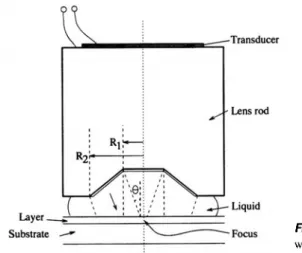
Very little has changed in spherical acoustic lens design since its first introduction. I 10) A high-performance lens (see Fig. 4.1) can be designed by finding

an optimum combination of cavity size, operating frequency, opening angle, antireflection layer, transducer size, and buffer rod length. An important aspect of the design is diffraction effects in the buffer rod when determining transducer size. A solution minimizing diffraction loss can be found in Ref. (II). The conven-tionallens has circular symmetry, and hence it is not expected to show sensitivity

~ ... .. .. . ---... - - - -_ ....

-transducer buffer rod Back Focal Plane Liquid q z

--- --- ---T/"'..

Focal plane

Figure 4. 1. Geometry of a spherical lens.

to the orientation of a particular surface of a crystalline object. However, since different surfaces of a crystal may have different reflection characteristics, the conventional lens can differentiate between grains on a polycrystalline object and generate a considerable contrast in acoustic micrographs. This sensitivity can be improved by a suitable selection of the transducer size and shape.(12) The resolution of images is determined mainly by the operating frequency and the opening angle of the lens. Since tilting the lens axis with respect to the object surface is equivalent to increasing the opening angle of the lens, it is possible to obtain an increased resolution in one direction, but this method is not very popular. In a multilayered solid structure, many leaky modes can be generated. A spherical acoustic microscope lens excites all these modes as long as they lie within the opening angle of the lens. The presence of many simultaneous modes clutters V(z) curves with such objects and makes interpretation difficult. Neverthe-less the spherical acoustic lens is still the most preferred lens design for imaging because of its good resolution performance.

To be able to compare lenses with different geometries, we write the specular reference component of the lens response in the following form:

VG(z) cos(2kz - wt) (1)

and the leaky wave component in the form

VR(z) cos(2kz cos

e, -

wt)

(2)

where

e,

is the critical angle; k is the wave number in the liquid medium; w is the carrier frequency;

z

is the distance between the focal plane and the object surface, increasing as separation between the lens and object increases; VG(z)

120

A. ATALAR, ET AL. and VR(z) are the normalized z variation of the specular geometric and leaky wave parts.8 While VGCz) has a maximum at focus point, z

=

0, VR(z) has a

maximum at some negative z. For substantial interference between these two components, nonzero values of the functions VG(z) and VR(z) should overlap in a wide range of z values. Obviously it is desirable to have large values for both. For a spherical lens, we can find the specular part by assuming a unity reflection coefficient and uniform insonification in the V(z) integral

where R is the reflection coefficient at the liquid-object interface as a function of the sine of the incidence angle;

ui

is the acoustic field at the back focal plane of the lens; P is the pupil function of the lens, which includes the transmission coefficient of the antireflection layer; q is the focal length of the lens; and ao is

the lens pupil radius. With paraxial approximation the integral becomes

f

"O

(-ikzr)

VG(z) = exp(2kz) 0 r exp ----;;- dr

(4)

Therefore VG(z) decays very rapidly as a sine function of defocus distance, in the form 1I1zl. The leaky wave part can be found by substituting

(k;,-k6)/(k~ - k;,) for the reflection coefficient R(kJk),IS'where k,> and ko are the leaky wave pole and zero

(5)

Figure 4.2 depicts numerically calculated VG and VR for a spherical lens at I GHz, with unity insonification and pupil function. The VG(z) is like a sine function as expected. It drops to - 35 dB level at z

= -

30 !Lm. When aluminum is chosen as object material, the leaky wave part VR(z) is -7.3 dB at its maximum. When sapphire is the object material, VR(z) has a peak of -26 dB. Since the signals are either very low or drop very rapidly, the conventional lens is not the best lens for characterization purposes.

Spherical Lens O,---,---.----.---.----r-~m_--._--_,

J\

5 ·10 ·15 :0-:9.·20 > ... Geometric Part .. Leaky Wave Part (AI) ••• Leaky Wave Part (sapphire)

-/ /

-:;:Ol\::i\

0

of\'

0 0 \ 0

f\

·35 / \

n

0,0 .'0 ".

Figure 4.2. Calculated geometrical and leaky wave parts of V(z) for a spherical lens (frequency,

f = I GHz; focal length, q = 115 ].1m; pupil radius, ao = 75 ].1m). Leaky wave parts are shown for aluminum and sapphire.

4.2.2. Lamb Wave Lens

The Lamb wave lens (see Figure 4.3) was introduced to increase the leaky wave content of the acoustic lens response.(13) It excites only one of the possible leaky modes at a time by generating conical wave fronts at a fixed incidence angle.(14) Rays emerging from the central flat portion of the Lamb wave lens are

incident normally onto the object surface, and they return to the lens to provide the reference VG(z) cos(2kz - wt) term given above. Since the critical angle of a layered material depends on frequency, it is possible to excite the leaky modes selectively by matching the fixed incidence angle with the corresponding critical angle at a particular frequency. Since most of the incident rays are at or near the critical angle, the conversion efficiency to the leaky mode is much higher than that of the conventional lens. Moreover the reference signal is higher than the reference produced by a conventional lens, and this signal does not decrease appreciably when the lens is defocused; in other words, Vdz) function is nearly uniform.

The Lamb wave lens can be used for imaging, since it provides a reasonable focusing performance. Furthermore subsurface images have a well-defined

coni-122

~ ... _~ _ _ _ -=::::::;-TranSducer Lens rod Liquid

E:::====~======

Substrate - ---~---A. ATALAR, ET Al.

Figure 4.3. The geometry of the Lamb

wave lens.

cal-focusing resolution, while corresponding images resolution obtained by the conventional lens is spoiled by aberrations due to refraction at the interfaces. We must note that the alignment of the Lamb wave lens with the object surface is difficult, since the flat part of the Lamb wave lens must be parallel to the object surface.

The V(z) measurement resulting from a center-blocked Lamb wave lens gives an interference-free curve (see Fig. 4.4). The peak at

z

= 0 is due to

specularly reflected rays. The second peak around z = -4 mm is created by

leaky waves. The minimum at

z

= -2.5 mm is due to destructive interference

between reflected and leaky waves, which are 1T out of phase. If waves incident

from the central portion of the Lamb wave lens are allowed to overlap leaky waves, an interference mechanism similar to the conventional lens results. For this purpose, the center of the lens should not be blocked. As depicted in Fig. 4.4, a V(z) curve with a good number of fringes is easily obtained. For large positive z values, no interference occurs. There the only contribution is from

the normal specular component (see Fig. 4.5). At points near z = 0, interference

results from the superposition of the normal specular component and the oblique specular reflection. The fringe period is determined by the cone angle of the Lamb wave lens, and it carries no or little information about the object. For more negative z values however, interference occurs between normal specularly re-flected rays and leaky waves. In this case, periodicity is determined by the leaky wave velocity of the particular mode. Figure 4.6 shows the calculated geometric

and leaky wave parts of V(z) for a Lamb wave lens for aluminum and sapphire.

As compared to a spherical lens, the leaky wave part is 6 dB greater for aluminum

and 20 dB greater for sapphire. Figure 4.7 depicts the V(z) variation for negative

2.0

1.0

o. 0 ~_L.----J,----1--':'--.J._--L_--L_---L_--L_--L_~'" 'L..c",-~~

-5 -4 -3 -2 -1 0 2 3 4 5 6 7

z (mm)

Figure 4.4. Lamb wave lens V(z) curves (center blocked and not blocked) for 0.6-mm copper on

steel (f = 9.6 MHz). Material parameters: Copper: VI = 5010 mis, v, = 2270 mis, p = 8.93 g/cml ; steel: V, = 5900 mis, V, = 3200 mis, p = 7.9 glcm3• Dashed line. center blocked; solid line, center

not blocked.

c:;:] .

_{, ... c:;:]}

" " I ' '. .

. .. .

.

. .... ... i

• ' 1 • • , >:::

l :,/

•

...

I ' I ,

c:;:] .

• • • I . I ' "

,,fiX ·\.l/v ...

[\!] . ,

z<o

124

A. ATALAR, ET AL. 0.0 00

.. · .. /···n·0··\···(\

-- --1',

(\\

-10.0

~

I

1\11

-10.0

I

1D 1D :!!- -20.0 :!!- -20.0 > > -30.0 -30.0 -40.0 L-_~~~~~_~,--_---' -40.0 L-~~",...-~--::"'-::-_----::--_-::! -30.0 -20.0 -10.0 0.0 10.0 -60.0 -40.0 -20.0 0.0 20.0 z (microns) z (microns)

Figure 4.6. Calculated geometric and leaky wave parts of V(z) for Lamb wave lenses designed for aluminum and sapphire objects (frequency, f = I GHz). For the first lens, R, = 15 11m, R2 = 30 11m. For the second lens, R, = 20 11m, R2 = 40 11m. Dashed line, leaky wave part; solid line,

geometric part.

0.5% perturbation in the shear wave velocity is readily detectable. With a 40-dB signal-to-noise ratio, it is possible to detect a velocity perturbation of 0.0075% in the layer material. With the same signal-to-noise ratio, a conventional lens with an envelope detector can detect only a 0.12% velocity perturbation.

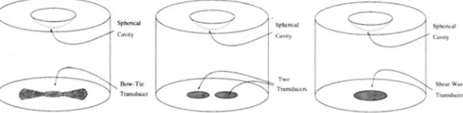
4.2.3. Directional Lenses with a Noncircular Transducer

To obtain orientation dependence, the circular symmetry of the lens must somehow be suppressed. It can be done on the transducer side by a noncircular-shaped bowtie,I'5) butterfly,I'6) rectangular, I 17) two separate,IIS) or shear wave

gener-ating transducersil9 , (see Fig. 4.8). The shape of the transducer may emphasize certain directions, even though diffraction effects in the buffer rod tend to smooth out directivity. A shear wave transducer has a polarization direction, and hence circular symmetry does not exist. Moreover with shear wave excitation instead of longitudinal waves, specular reflection contribution at the output can be mini-mized. With such a lens, there are no incident rays normal to the object surface.120)

When such a lens is moved out of focus, the only contribution to the output is from leaky waves. However the output signal is rather dull, since there is no interference. All of these lenses have good resolution performance, and they can be used as imaging lenses. But diffraction in the lens rod limits their use as accurate characterization tools. Differential phase contrast lensl2l.22) can also be considered in this class.

2.0 ,---r---r---.---.,

~

10

0.0

-5 -4 -3 -2 -I

z (mm)

Figure 4.7. Lamb wave lens V(z) curves for copper on steel (solid) and for a copper layer c., perturbed by 1% (dashed) (f = 9.6 MHz).

4.2.4. Line Focus Beam Lens

Kushibiki and coworkers proposed and used an LFB acoustic lens. The virtues and limitations of this lens are extensively described in the literature.<2J-26) Such a lens is formed by a cylindrical cavity in the lens rod (see Fig. 4.9).

Generated rays hit the object surface in the same azimuthal plane, so leaky waves

...

Sptcna.1

""'-'

C"~lt ) _Y'III) (

....

) T ••

Dow·Ti<-TIllModIlt.rn. Sk.ar 'lI> .~'C'

T.--da:.t:r _{'Tr:oMdU('(',}

126

H Cylindrical Cavity A. ATALAR, ET AL. Figure 4.9. FB lens.

in that plane affect the response of the lens. This lens has poor resolution in one direction, and it cannot be used for imaging, but it has very good directional sensitivity, and it is suitable for characterizing anisotropic crystals.(27) Aligning the lens with the surface is more difficult compared to the conventional lens because the line focus must be parallel to the object surface. To compare the LFB lens with the conventional lens, we must determine the specular and leaky wave amplitudes. An expression for the geometric part VG(z) can be written as

A paraxial approximation shows that VG(z) decays as 11

Fz,

and hence more slowly than the spherical case. The leaky wave part can be estimated from

(7)

Note that these formulas differ from spherical lens formulas solely in the factor of r inside the integral. That factor exists in the spherical lens case due to the circular nature of the geometry. Figure 4.10 shows calculated VcCz) and VR(z)

·15 :0 ~·20 >

,

·25 . I I I

,

I If·

,

I I ·30 I '.

,

" If ·35

,

I,

.4g

_{. 0 ·25 ·20} I I

,

, I _,-I

,

I

,

,

I ' I

,

·15 ·10 z (microns) ·5

o

I

I"

I I I \' \ f\ I I I \1 \ 1\ I' 5 10

Figure 4.10. Calculated geometrical (solid line) and leaky wave parts of V(z) for an LFB lens

(f = I GHz, q = lIS fL, all = 75 fLm). Leaky wave parts are shown for aluminum (dashed line)

and sapphire (dotted line).

smaller than the spherical case, as expected from geometrical considerations.

*

But, the geometric part is larger. The oscillations in the leaky wave part can be attributed to diffraction effects. LFB lens generates extended V(z) interference and gives excellent characterization performance.

4.2.5. Slit-Aperture Lens

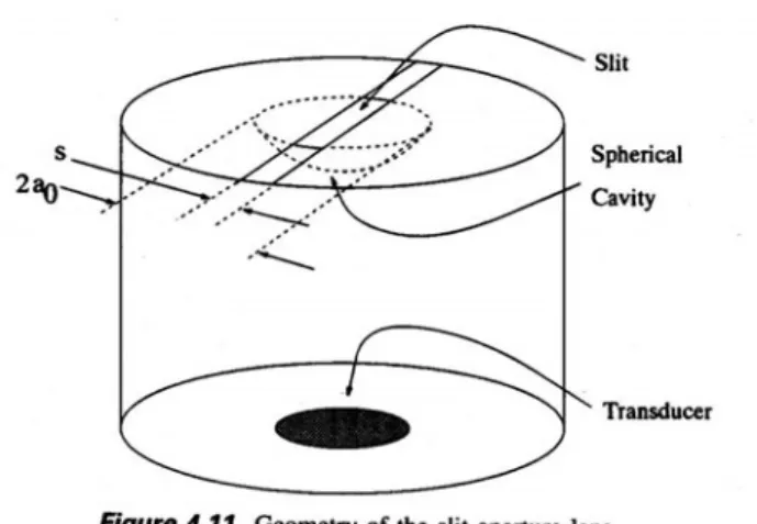
Lenses providing directionality in the transducer shape suffer from a diffrac-tion effect in the buffer rod and provide only limited direcdiffrac-tionality, not sufficient for accurate measurement. If directionality is introduced in the lens pupil plane, diffraction in the lens rod plays no role. A slit aperture can be formed easily, and it provides sufficient directionality.,2x, Figure 4.11 shows the geometry of the slit-aperture lens. It consists of a conventional acoustic lens with a specially designed aperture in front. The slit is formed by parallel edges of two absorbing sheets. The distance between the sheets determines the slit width. The directional *The fraction of incident power that can be coupled to the leaky waves is 21TallD.hra~ = 2D./all for the spherical lens and 2HD./2Hao = D./ao for the LFB lens, where D. is the width of the narrow strip in the pupil function responsible for leaky wave excitation. Here the lens opening angle is chosen to be just sufficient to excite leaky waves.

128

Slit Spherical Cavity A. ATALAR, ET AL. Transducer

Figure 4.11. Geometry of the slit-apenure lens.

knife-edge-aperture lensl291 _{is essentialJy equivalent to this lens when the knife} edge blocks less than half of the pupil. The parameter s is then twice the distance between the knife edge and the pupil center.

A diffraction-corrected ray theory approach for the slit lens is given in Ref. (30). Although the ray theory provides very valuable physical insight into the problem, it cannot handle the problem correctly near the focus point, and it gives only an approximate solution. Here we give an expression for the slit-aperture lens V(z) using the angular spectrum approach.13ll

V(z) =

ro

R,(~)[ui(r)Fexp[i2kzJl

-

(~)2]

dr (8)

where

(9)

Here Re is the average reflection coefficient of an anisotropic material as a function of the sine of the incidence angle. For a slit lens, the pupil function can be written as

P(x,y) =

g

if

Ixl

<

sl2

otherwise

and

(10)

where s is the slit width and ao is the lens aperture radius. Note that the apodization effect caused by the matching layer on the lens can be included in the function

Calculating the reflection coefficient at a liquid - anisotropic solid interface is not a trivial procedure, since an analytic expression does not exist. Therefore numerical methods are used to calculate it.(32-34) In its most general form, the anisotropic solid is represented by its 21 elastic constants, so materials with arbitrary orientation can be handled by transforming the stiffness matrix by multiplying with Bond matrices.

We have calculated the V(z) response of a slit-aperture lens with the follow-ing parameters: Operation frequency of 200 MHz, lens cavity radius of 500 /Lm, lens aperture radius ao

=

435 /Lm, transducer radius aT

=

435 /Lm, lens buffer rod length L

=

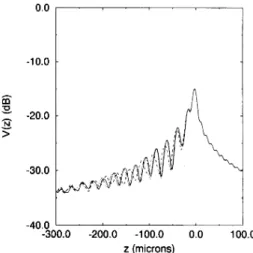
tOmm. Slit width s was kept as a variable parameter. Various single-crystal solids are considered. Figure 4.12 shows the calculated V( z) curves for a GaAs substrate (001) surface. Different curves are for different orientations of slit with respect to crystal symmetry axes. For a slit width equal to one-tenth of the lens aperture, the loss in the signal level is about 15 dB. Figure 4.13 depicts a similar set of V(z) curves for the (111) surface of GaAs. Calculations are repeated for different slit widths. As the slit width is increased, the resulting

V(z) curves converge to each other for different orientations of an anisotropic

crystal. As the slit width is reduced, there is a loss in the signal output level, but different orientations have different responses.

Figure 4.14 shows the results of simulations for varying slit widths for a GaAs (111) surface. In the same figure, the actual SAW velocity is indicated as a function of propagation direction. For slit widths less than 5% of the aperture size, the extracted velocities follow the actual velocity curve closely. But as slit size increases, the error between the estimated and actual velocities increases very rapidly. When the slit size is greater than 20% of the aperture size, estimates are quite unreliable.

Figure 4.12. Calculated V(z) curves for GaAs (001) surface at various directions with a slit-aperture lens. S = 0.1 a; solid line, 0 degrees; dotted line, 15 degrees; dashed line, 30 degrees.

[C :8-E > -10.0 -20.0 -30.0 -40.0 '---~~-~~-~~---' -300.0 -200.0 -100.0 0.0 100.0 z (microns)

130

A. ATALAR, ET AL.

-10.0

-20.0

-30.0

Figure 4.13. Calculated V(z) curves for a GaAs (Ill) surface at various directions -40.0 L---_ _ ~ _ _ ~ _ _ ~ _ _ ~ with a slit-aperture lens. S = O.lao; solid

-300.0 -200.0 -100.0 0.0 100.0 line, 0 degrees; dotted line, 10 degrees;

z (microns) dashed line, 20 degrees.

4.2.6. V-Groove Lens

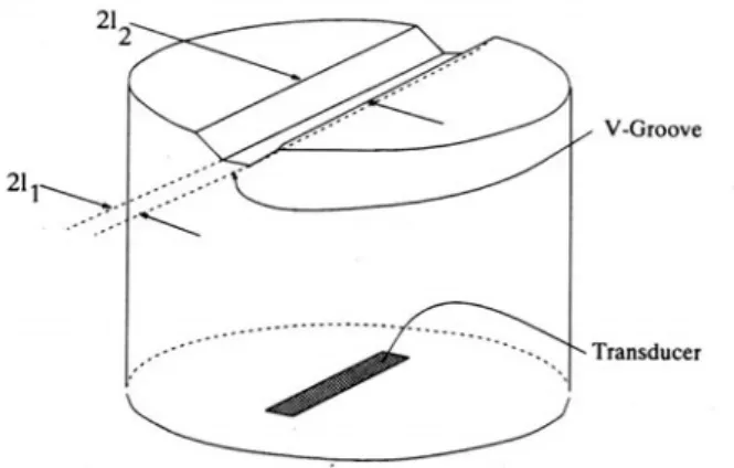
The V -groove lens is a combination of an LFB lens and the Lamb wave lens.(35) It inherits the high efficiency of the Lamb wave lens, while providing the high directionality of the LFB lens. The V -groove lens differs from the LFB lens in the way the refracting element of the lens is fabricated. Unlike the cylindrical cavity of the LFB lens, the V -groove lens has a V -shaped groove with a flattened bottom, as shown in Fig. 4.15. Essentially, the relationship between an LFB lens and a conventional lens is the same as the relationship between the V -groove lens

u

i

€

_o ~ 2700.0 ,---~---, - - Actual - - s=0.025a 5=0.05 a ---. 5=0.075 a 2600.0 ---- 5=0.1 a 2500.0

2400.0 L---_ _ _ ~ _ _ _ ~ _ _ ---...J Figure 4. 14. Actual and estimated

veloci-0.0 10.0 20.0 30.0 ties on a GaAs (Ill) surface as a function

21,---..,. .. ' .:::::: ..

...

:.:.-<-V-Groove

Transducer

Figure 4.15. Geometry of the V-groove lens.

and the Lamb wave lens.(3) In other words, leaky waves are selectively excited on the surface of the object when a V -groove lens is used, while in the case of an LFB lens, all modes are excited due to its wide angular spectrum.

The transducer is designed to insonify a substantial portion of the groove with a minimal waste of power elsewhere. The flat bottom part does not cause refraction, and thus a part of the incident beam insonities the object surface at normal incidence. Symmetrical sides of the groove cause a refraction, and hence two symmetrical beams insonify the object surface at the same incidence angle. The interference of the refracted beams, which encounters leaky wave modes on the object surface, with the reference beam resulting from the specular reflection of the normally incident beam produces the V(z) . A good match between the median direction of the refracted beam and the critical angle for the object improves measurement accuracy.

Simulating the performance of a lens involves propagating acoustic waves between the transducer and the refracting element. The wave front is then propa-gated through the refracting element using ray theory. The wave front is reflected from the object surface on propagation in liquid. This analysis is similar to the one developed for the Lamb wave lens,(3) except for the circular symmetry. While the circular symmetry of the Lamb wave lens allows the use of a fast Hankel transform for propagation purposes, the propagation problem in a V-groove lens requires the more costly two-dimensional Fourier transform (FFT).

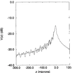
Lens alignment is achieved easily by maximizing the signal from the flat part of the lens, since the maximum signal is reached when the object surface is perfectly parallel to the flat part of the V -groove. A simulated V(z) curve for a V-groove lens with the (001) surface ([100] propagation) of silicon as the reflector is depicted in Fig. 4.16 with experimental measurements.

132

-5.00 10 ~

8:

> -10.00 - Theory Go- 0 Exp data

-15.00 L...~~ _ _ -'-'L-_~~_~-.J

-6.000 -4.000 -2.000 0.000 2.000 Z (mm)

A. ATALAR, ET AL.

Figure 4.16. Calculated (solid line) and measured (dotted line) V(z) values along [100] direction on (00 I)

surface of Si at f = 25 MHz for a V -groove lens.

To compare the performance of the V -groove lens with other lenses, geomet-ric and leaky wave parts of a received signal are calculated for typical lenses. Figure 4.17 is a plot of the results. Obviously the geometric part is much greater than either the LFB or the spherical lens. The leaky wave part is about 12 dB greater than the LFB lens.

-5 .-- (\, i

.···-·---n/\

'(,

r\

·5

p (\ (\\

. \ /', (\ II

1/')

·-iP·--.l,,!

·10

_J

d \

f i,l I,

'It

10 _--.- . I ' \ i , i 'I} ·15

\, II

Ii

I

I

·15 V I,

"

~

II

I

iii

II

:2.·20 £-20 _\, > 'j

I

> ·25 -25 I I ·30 ·30 ·35 ·35 -40 _·40 ·30 .2D ·10 10 ·40 ·100 ·80 ·60 ·40 ·20 z (microns) z (microns)

Figure 4.17. Calculated geometrical (solid line) and leaky wave (dashed line) parts of V(z) for V-groove lenses designed for aluminum (right) and sapphire (left) objects (f = I GHz). (a) I, = 14 fLm, I~ = 36 fLm. (b) I, = 22 fLm, I~ = 60 fLm. Diffraction effects are neglected.

4.3. Comparing Signal Processing Electronics

In this section we compare various signal-processing systems presently in use for acoustic microscopy. To be able to compare them quantitatively, we define a figure of merit and calculate it for all systems under similar conditions. A white gaussian noise n(t) with noise power W is considered. We find the response of the particular configuration with respect to variations in the critical angle and surface topography.

4.3.1. Conventional Envelope Detection System

The conventional acoustic microscope system shown in Fig. 4.18 uses an envelope detector to obtain the output signal. Such a detector can have no sensitivity to the phase of the received signal. This is not a great disadvantage, since the microscope output signal is the result of an interference anyway. The low-pass, filtered linear envelope detector output can be written as

V(z) = LPF{ Ivc(z) cos(2kz - wt)

+

VR(z) cos(2kz cos 0, - wt) (II)

+

n(t)l)

where n(t) denotes the noise and LPF [.] the low pass filtering operation. A typical V(z) curve is shown in Fig. 4.19. Quantitative object parameters can be deduced either by an inversion integral applied to the V(z) data(36) or by Fourier transformation of data points to determine the characteristic periodicity. (24)

4.3.2. Amplitude and Phase-Measuring Synchronous Detection System

It is possible to detect the phase of an acoustic microscope output voltage with a phase-sensitive receiver system.(37 ) In such a system, the received signal is multiplied with a reference signal obtained from the carrier (see Fig. 4.20).

Figure 4.18. A conventional acoustic micro-scope system.

RF

134

A. A TALAR, ET Al. 800.0 I"" \ , , , , , , , 0.0 ,

\

/'''\ _,

_!

, " , '\\ 1'1'-.... \ !

\

I ,/" ; _'" ; -,

--

, '\ _I , /

\

' ,

/

' , , , , ,

'hif

I

'}\/K

'-rI

V

vv ~

VV

_V 400.0 -400.0 -800.0 -15.0 -10.0 -5.0 0.0 5.0 z (microns)

Figure 4.19. V(z) curvcs for aluminum for conventional (dotted line) and phase-measuring (solid

line) systems (f = 1100 MHz).

Phase Sifter

Figure 4.20. A phase-measuring acoustic

Low-pass, filtered mixer output gives a voltage highly sensitive to the surface topography of the object material. This signal can be expressed as

V(z)' = Vc(z) cos(2kz

+

1jI)

+

VR(Z) cos(2kz cos 9,

+

1jI)

+

n,(t) cos IjI

(12)

where nJt) is the in-phase component of the noise and IjI is the phase shift of the carrier. The output voltage varies sinusoidally with distance with an envelope that is the same as that obtained from the conventional system (see Fig, 4,19). If IjI is changed in small steps and the output signal is measured, it is possible to find the complex amplitude of the signal. With suitable averaging methods, it is possible to detect surface height variations less than 1/500 of the wavelengthl3Hl or to measure residual stressesY9l

4.3.3. Conventional System with Added Carrier

A conventional system with a reduced onloff ratio in the pulse generation electronics may result in a phase-sensitive system without the extra cost of phase-measuring electronics. In this case, carrier leakage causes a pseudo-phase-sensitive system. This leakage can be introduced intentionally in a controlled manner (see Fig. 4.21), After detection the output signal contains components that vary sinusoidally as a function of z, the lens object separation in Fig. 4.22. The resulting envelope detector output is written as

V(z)

=

LPF{ \Vdz) cos(2kz - wt)

+

VR(z) cos(2kz cos 9, - wt) (13)

+

C cos(1jI - wt)

+

n(t)\}

where C is the magnitude of the leak component and IjI is its phase. If the amount of leakage can be varied, a maximum sensitivity can be reached,

Figure 4.21. A conventional system with

136

~ CIl ..,

a

::l

'"

...

'"

...

.., .0

_...

~ N ;;-A. ATALAR, ET AL. 8000 '---~---"---~---"'---~---r--~---' 400.0 00 ,---,' -400.0 , , , _{, , , ,} , , _, , , , _{, , ,} , _{, ,} " -800.0 L-_ _ '--_--.J _ _ - ' _ _ --'. _ _ ~ _ _ ___'_ _ _ _'_ _ _ _' -15.0 -10.0 -5.0 0.0 5.0 Z (microns)

Figure 4.22. V(z) curves for aluminum for a conventional system with some added carrier (solid line) and a differential phase system (dashed line) (f = 1100 MHz).

4.3.4. Differential Phase System

Phase-measuring systems previously described suffer from some problems that reduce measurement accuracy. Such external factors as vibration of the mechanical-scanning stage or temperature fluctuations in the coupling medium result in phase errors. These phase errors reduce the accuracy of quantitative measurements. To isolate the external factors, a reference signal that undergoes the same phase fluctuation may be used. This reference may be the specular reflection component. The procedure is to separate the specular and leaky wave contributions in the time domain and to multiply these two signals after proper delay (Fig. 4.23). Low-pass filtered mixer output can be given as

v

=

VG(Z)VR(Z) cos[2kz(l - cos 8,.)]

+

noise (14)

This setup provides excellent sensitivity to material properties, since it can measure small variations in the phase of leaky waves. In addition to having a

Figure 4.23. A differential phase-measur-ing acoustic microscope.

Phase shifter

reduced sensitivity to external factors, it is insensitive to small surface height variations. As shown in Fig. 4.22, the output signal is predominantly determined by object-elastic properties. The greatest difficulty is to separate these two signals in the time domain. For this purpose, lenses must have wide bandwidths to pass short pulses, and a substantial defocus is necessary, causing a loss in resolution. Special geometries involving shear wave or mixed-mode transducers can be employed to obtain separated pulses without a great resolution sacrifice.(40)

4.3.5. Comparing Systems

We can compare the performance of these schemes in the presence of noise for either critical angle measurement or surface topography. In the first case, we define a figure of merit FMB as

(aVlaOJ2

FMB=

-(No

*

S N RJ (15)

where S N R; is the signal-to-noise ratio defined as total power input to the lens

divided by noise power W. The No is the output noise power; No may contain

signal cross noise terms depending on the processing scheme employed, and in general it is not equal to W. This figure of merit indicates how sensitive the

system is as a function of critical angle at a given defocus. Moreover it includes the effects of the presence of noise. In the second case, we define another figure of merit, FM" which shows the sensitivity with respect to surface height z.

FM

=

[(I)aVl2k(az)F

Z (No

*

S N R;)

(16)

We assume a unity total input power with a sufficiently high signal-to-noise ratio. In the carrier-added system, the added carrier amplitude is much higher than other signal components. The choice of <I> and z is made such that expressions

138

A. ATALAR. ET AL. are simplified and figure of merit values are maximized. The results are presented in Table 4.1 in terms of a normalized geometric part VG, a leaky wave part VL,

and the critical angle (le. Inspecting the FMe formulas indicates that critical angle

sensitivity grows as

Ikzl

is increased. Moreover higher critical angles result in more sensitive systems. The synchronous system is the best. The carrier-added system approaches the performance of the synchronous system if the added carrier is sufficiently large. The envelope detector system is the worst. In all cases, increasing the geometric part and the leaky wave part is rewarding. Formulas for FM, show that the synchronous system also gives the best z sensitivity. The least sensitive system is again the envelope detection scheme.

We used these formulas and typical VG and VL values for different lens geometries. Tables 4.2 and 4.3 give typical values assuming a large signal-to-noise ratio at the input. This assumption makes sure that the envelope detector operates above the threshold.

Results show that the best system for critical angle measurement is the synchronous detection scheme. All other systems have similar but lower figures of merit. The conventiollal envelope detection system performance deteriorates according to the expression given in Table 4.1 as the input signal-to-noise ratio falls below the detector threshold. Moreover the nonlinearity of the detector diode may introduce some errors in quantitative measurements. For low signal levels, dropping below the threshold can be avoided by increasing the added carrier amplitude. Synchronous detector and differential phase systems, on the other hand, maintain the same figure of merit even for small input signal levels. The differential phase system is inferior to the synchronous detector, since what may be considered as the carrier is also corrupted with noise. As already men-tioned, the differential phase system gives the highest performance configuration because of its relative insensitivity to external factors.

As far as measuring surface topography is concerned, the synchronous system is the most sensitive by a large margin. It is followed by the carrier-added envelope detector scheme. The other two methods are relatively insensitive to surface topography. In those systems, reduced leaky wave contribution results in diminished z sensitivity.

Although the synchronous detection scheme gives the best figures of merit, implementation cost is high. The envelope detector with carrier-added provides

Table 4.1. Figures of Merits of Different Signal-Processing Systems with Respect to Critical Angle

and Topography System Envelop detection Carrier added Synchronous Differential phase

FM, (Critical angle figure of merit) VbVU2kz sin flY/(Ve + V,)'

< Vb(2kz sin 8,)' VWkz sin flY VbVi(2kz sin !l,)'/(Vb + Vi)

FM, (Topography figure of merit)

Vb Vi(l - cos 8,)'/(vc; + V,J'

< (Ve; + VL cos 8,),

(Ve; + VL cos 8,)'

Table 4.2. Typical Critical Angle Figure of Merit Values for kz = 27-rr and

e,

= 30a

System Sphericalb Lamb'

Envelope detection 0.034 0.84

Synchronous 0.84 3.4

Differential phase 0.049 1.7

'These are typical values when aluminum is used as the object. 'For a spherical lens: VG = 0.05, VL = 0.2.

'For a Lamb wave lens: VG = 0.4, VL = 0.4.

"For an LFB lens: VG = 0.2, VL = 0.14.

'For a V -groove lens: VG = 0.4, VL = 0.5.

FMe

LFBd V-Groove'

0.14 1

0.41 5.2

0.28 2

a significant improvement over the conventional system with little or no cost. Expressions given for FMe indicate that a large defocus factor kz is preferable.

In all cases, figures of merit improve sharply with increased leaky wave signal amplitude. Therefore lens configurations maximizing this amplitude have higher figure of merit regardless of the detection scheme employed. However when the leaky wave signal is comparable with the geometrical signal, analysis of V(z),

based on a linear approximation can no longer be used.(41)

4.4. The

V(f)

Characterization Method

In Section 4.4 we describe an alternative to the V(z) characterization tech-nique. This method is applicable to acoustic lens systems with restricted angular coverage and a reasonable frequency bandwidth. The output voltage of a Lamb wave or a V -groove lens recorded as a function of frequency results in a unique curve [V(f)].(l4) Excited leaky modes reveal themselves as peaks in the V(f)

curve at frequencies where the critical angle of the mode matches the fixed incidence angle of the lens. Since the excitation frequency of leaky modes is highly dependent on elastic parameters of the layers and the bond quality at interfaces, peak positions in the V(f) curve are very sensitive to these parameters.

Table 4.3. Typical Topography Figure of Merit Values for

kz = 27-rr and

e,.

= 30

System Spherical Lamb

Envelope detection 0.000028 0.00071

Synchronous 0.049 0.56

140

A. ATALAR, ET AL. A typical V(f) curve for a center-blocked Lamb wave lens is shown in Fig. 4.24.

If the center is not blocked, a more interesting V(f) curve results. As depicted

in the same figure, this curve has an interference pattern that results in high sensitivity. Since a signal is now present even in the absence of leaky waves, a background level always exists. This background level can be avoided if the specular and leaky wave components are separated and mixed with each other. Separation can be achieved in the time domain. As plotted in the same figure, this pattern is free from background while maintaining high sensitivity.

For the purpose of investigating the performance of the Lamb wave lens in a layered structure, a sample composed of silver and copper layers on a steel substrate is considered. Dispersion characteristics of this structure, with perfect bonds at the interfaces, is depicted in Fig. 4.25. The vertical axis shows the incidence angle in a water medium for which the best excitation of a particular mode is achieved. It can be observed that two modes can be excited at approxi-mately 35° in the frequency range of 4-9 MHz.

1.5 1.3 1.1 0.9 0.7

-

0.5 ':> 0.3 0.1 -0.1 -0.3 -0.5 4.0 6.0 8.0 10.0 f (MHz) 12.0 14.0

Figure 4.24. V(f) curves for O.6-mm copper on steel using different Lamb wave systems. Dotted

45 Q) 1: 40 ~ wedae anale ~ Q) 'On 35 .: C1l -;; () ~ 30

_...

u

Figure 4.25. Dispersion characteristics of

modes in a multilayered structure composed of 90 microns of silver and 505 microns of copper on steel substrate. A 35.8° wedge angle shows the angle of incident waves generated by the Lamb wave lens used in experiments.

4 5 6 7 8 9 10 11 12

f (MHz)

A better understanding of the reflection phenomenon in layered materials can be achieved by decomposing the reflection coefficient R into two parts(SJ: A surface reflection coefficient R, and a subsurface reflection coefficient Ru' The

K

is due to the interface between the liquid and the topmost layer, excluding effects of leaky waves and subsurface layers. This part is found by considering a half-space made up of the same material as the topmost layer, with the leaky wave component suppressed by setting phase variation in this reflection coefficient to zero(42)

K

=

\RT\

where

RT

is the reflection coefficient between the liquid and the half-space made up of the topmost layer material. The subsurface reflection coefficient is found by subtracting the surface reflection coefficient from the original, Ru

=

R - R,.

The subsurface reflection coefficient includes effects of leaky waves as well as subsurface specular reflections. Figure 4.26 depicts the magnitude of the calcu-lated subsurface reflection coefficient for the material just described. Leaky waves, such as leaky Rayleigh, leaky Lamb waves, and lateral waves, emerge as peaks at corresponding incidence angles. The magnitude of the peaks can be greater than unity but always less than or equal to 2. This is due to opposing phases of the surface and subsurface reflection coefficients. Peaks arise from Lamb and lateral waves. The width of the peaks indicates the angular spread within which the mode can be efficiently excited. This in tum determines the aperture size of the Lamb wave lens for the most efficient excitation.

Peaks in the V(f) curve are related to particular Lamb wave modes. We

may suspect that each of these modes is predominantly present in one of the layers of the multilayered structure. To determine the validity of this hypothesis,

142

0.0 20.0 40.0 60.0

Incident Angle (degree) 80.0

A. ATALAR, ET AL.

Figure 4.26. A subsurface reflection co-efficient for the multilayered structure composed of 90-fJ,m Ag and 505 fJ,m of Cu on a steel substrate at 7.8 MHz.

we calculated the lateral component of the Poynting vector for plane wave excitation for various critical angles. The poynting vector is a measure of energy flow. Figure 4.27 shows the results for a multilayered structure under two different excitation angles. There is a concentration of acoustic energy along particular interfaces. Hence different interfaces are responsible for modes at these two angles. Once this relationship is ascertained, images obtained from these modes can be attributed to those interfaces. Therefore the Lamb wave lens has the inherent ability to generate selective interface images.

The effectiveness of a Lamb wave lens using the V(f) technique for

quantita-tive characterization can be evaluated for the sample described in the previous section. Figure 4.28 depicts the calculated V(f) curve and measurements for the

case when both bonds are perfect. Measurements are performed by using a Lamb wave lens that has the same wedge angle of 45.9°. A very good agreement is obtained between experiment and theory. The V(f) measurements and calculated

curve for a region with a disbond in the upper interface is given in Fig. 4.29. A slight shift can be observed in the curve as expected. The effect of a disbond in lower interface on Vet) can be observed in Fig. 4.30. The central mode is now reduced to 7 MHz.

We may exploit the sensitivity of the Lamb wave lens by generating a peak frequency image (PFI) , which is obtained by mapping the peak frequency of a

particular leaky mode at every point in the form of an image. The PFI provides information directly about the spatial variation of parameters of the layers and the bond quality at interfaces. Considering that each layer and interface in a multilayered material affect these modes in a different manner, the effect of each parameter at a desired layer and interface can be selectively observed and

0.0 rr---.-==--~---__,_---~--___, Al -02

eu

S

.§. :!

..

-0.4

"

..

.,

Al E

"

5 0

..

_{5 -06}

"

... Fe c !! !!l c -08 -10 L -_ _ ~ _ _ _ --'-_ _ _ ~ _ _ _ __'_ _ _ _ ~ _ _ ___' 0.0 100 20.0 30.0

Poynting vector lateral component

Figure 4.27. The lateral poynting vector component as a function of distance in the three-layer

material. f = 7 MHz; thin line, theta = 28.4; heavy line, theta = 32.6.

Figure 4.28. Measured (squares) and calculated (line) V(f) curves (good bond) for the Ag-Cu-steel sample.

~

....

:;-100 80 60 40 20 0 5

'.

'. 6 7 8 9 f (MHz)

144

A. ATALAR, ET Al. 80 r---.---~-,---,---, 60

_.'.

.

...

!,. 20

o

'---'---'.~---'---' Figure 4.29. Measured (squares) and

5 6 7 8 9 calculated (line) V(f) curves (disbond at

f (MHz) upper interface) for the Ag-Cu-steel _sample.

characterized by the Lamb wave lens. The PFI images can be obtained very fast because there is no need to scan the object in the z direction, an operation that is inherently very slow. This mode of imaging is preferable, since it reduces the ambiguity that may arise in conventional imaging, where changing z may cause contrast reversal. Figure 4.31 shows a PFI image obtained from a Lamb wave lens for a copper layer on steel where a slippery bond (disbondy43) is intentionally induced in a restricted region. This region shows up with a high contrast in the image. 80 .---r---,_---,---, 60

."

. .

. .

".r 20

.'

.' "

...

'

...

..

,

.

'I.

1-o '---'-_____ '--___ --'-___ ---"

Figure 4.30. Measured (squares) and

5 6 7

f(MHz)

8 9 calculated (line) V(f) curves (disbond at lower interface) for the Ag-Cu-steel sample.

Figure 4.31. The peak frequency image of a 0.6-mm thick copper layer on steel obtained by a Lamb wave lens. Frequency range is 7.2-8.7 MHz. The interface contains an intentionally generated disbond region. Image dimensions are 20 mm by 20 mm.

4.5. Accuracy of Velocity Measurement Using the V(z) Method The LFB, slit-aperture and V -groove lenses are primarily used to determine leaky wave velocities on anisotropic material surfaces. Spherical and Lamb wave lenses can also be employed for similar purposes when the material is isotropic. The V(z) curves obtained by these lenses are analyzed and velocities are found. The procedure for extracting velocity information(41) from V(z) can be summarized as follows

• Obtain V(z) for the object.

• Obtain Vrej(Z) for the same object with its reflection phase zeroed. Experi-mentally Vrer(Z) can be obtained by using Pb as the object.

• Find V2_{(z) - Vlrej(z). If the leaky wave content is small, V(z) - Vrej(Z)}

can be used instead.(23) • Pad data with zeroes.

146

A. ATALAR, ET AL. • Apply FFT to find the period of oscillation .

• Determine velocity from the period.

To deduce the absolute accuracy of this method, we performed a series of simulations for LFB and V -groove lenses. As the object material, we used a number of isotropic crystals whose elastic constants are known. From the known constants of crystal and liquid medium first, we determined the leaky surface wave velocity. This involves calculating complex poles of the reflection coefficient. Calculated Rayleigh velocity values are shown in the first column of Tables 4.4 and 4.5. Then we tried to find the same velocity using the V(z) method. The V(z)

responses are calculated from the known elastic parameters of the materials and the known geometry of the lenses. These responses are then input into the velocity extraction algorithm using the FFT method.(23) Calculations are made under vari-ous assumptions. First uniform insonification of the lens is assumed. Then the actual field pattern calculated by using diffraction effects in the buffer rod is used. Finally the reference material is chosen as Pb rather than the phase-zeroed reflection coefficient. Different assumptions result in slightly different estimates. Extracted velocities are then compared with velocities computed directly from elastic parameters. Error values are tabulated in the same tables. Obviously our simulations do not include effects of mechanical and measurement inaccuracy in the

z

direction, object surface alignment error, electrical noise and temperature change that normally occur in an actual experiment. In that sense, our accuracy estimations are optimistic.

Results indicate that we may have an error on the order of 1 % in either direction. The errors that we find here are somewhat less than the experimental absolute errors reported by Kushibiki and others(441, as expected. However, our findings show that errors cannot be corrected simply by a bias argument based on measurements from standard specimens. The error figures reported in Ref. 44 are very close to each other, since materials under investigation are very similar to each other with similar leaky wave velocities. Since the direction of

Table 4.4. Absolute Errors Using LFB Lens for Different Materials under Different Assumptions"

Uniform Ideal Pb

Material Actual field Error reference Error reference Error

Aluminum 2858.6 286l.l 0.08% 2863.6 0.17% 2862.0 0.12%

Chromium 3656.7 3660.0 0.09% 3669.3 0.34% 3665.0 0.22%

Alumina 5679.0 5696.6 0.30% 5706.4 0.48% 5608.2 -1.25%

Silicon carbide 6809.5 6850.1 0.60% 6884.8 1.11% 6672.4 -2.01%

"Actual velocities (first column) are compared with V(z)-extracted velocities under a uniform field (second column), rcal field with ideal reference reflector (fourth column), real field with Pb as reference reflector (sixth column) assumptions.

Table 4.5. Absolute Errors Using V-Groove Lens for Different Materials under Different Assumptions"

Uniform Ideal Pb

Material Actual field Error reference Error reference Error

Aluminum 2858.6 2854.3 -0.15% 2848.8 -0.34% 2846.3 -0.43%

Chromium 3656.7 3654.0 -0.07% 3650.3 -0.18% 3642.9 -0.38%

Alumina 5679.0 5665.6 -0.24% 5636.3 -0.75% 5659.3 -0.35%

Silicon carbide 6809.5 6810.5 0.01% 6792.3 -0.25% 6741.7 -0.9l!%

"Actual velocities (first column) are compared with Viz) extracted velocities under uniform field (second column). real field with ideal reference reflector (fourth column), real field with Pb as reference reflector (sixth column)

assumptions.

error changes for varying leaky wave velocities, a simple multiplicative error correction is obviously not possible.

The reason for the existence of this systematic error can be attributed to asymmetry in the contribution of the leaky wave pole-zero pair. This asymmetry is especially pronounced for Lamb wave or surface-skimming mode phase transi-tions,(45) but it exists even for the simple Rayleigh wave mode. Hence error levels given in Table 4.5 can be considered as the lower bound for the absolute error. A correction factor can be applied for each measurement if an error simula-tion is performed for the lens and material under considerasimula-tion. The correcsimula-tion factor is not fixed, but rather depends on sample parameters.

Table 4,6 summarizes simulation results for a slit lens with s

=

0.1 a.

Various single crystals with different cuts along various propagation directions are considered. Table 4.6 shows the percentage difference between the

V(z)-extracted velocity and actual velocity as absolute error. Simulations are done for a slit lens with s

=

O.la. For most materials, the error is about I %. Repeatability of experiments can be much better for each of the techniques than the values given in Table 4.6.

Table 4.6. Calculated Wave Velocities versus Actual Velocities with Slit-Aperture Lens (s = O.la)

Material Cut Direction Actual V, Extracted V, Error (%)

Al 011 0 2973.5 3008.1 1.16 Al III 0 2841.2 2869.5 I GaAs 011 0 2813.7 2831.8 0.64 GaAs III 0 2433.8 2443.6 0.41 Si 011 0 5010.4 4994.1 -0.33 Si 011 10 4991.5 4970.3 -0.43 Si 011 20 4936.5 4900.8 -0.72 Si 011 30 4850.0 4812.7 -0.77

148

A. ATALAR, ET AL. 4.6. Conclusions

We compared various lens designs and signal-processing systems used in acoustic microscopy. The conventional spherical lens offers the best resolution performance, but it has an inferior characterization ability. The circular symmetry of this lens makes only isotropic material characterization possible. An empha-sized leaky wave contribution and hence a higher figure of merit can be obtained by a Lamb wave lens at the expense of a limited range of measurable object velocity. It is possible to measure perturbations in the object parameters at least an order of magnitude smaller than possible with conventional lens. The Lamb wave lens has an additional advantage: Possible modes can be separated by proper choice of frequency and/or cone angle.

The LFB lens has a directional sensitivity, hence it can be used to characterize anisotropic substrates. But it has poor resolution in one direction and a slightly lower figure of merit, since the leaky wave component is smaller in amplitude compared to the conventional lens.

The slit-aperture lens is a compromise between characterization accuracy and good resolution. Unlike the LFB lens, it can be used as an imaging lens while providing a directionality for velocity measurement. The usefulness of this lens is limited by its low signal-to-noise ratio.

The directional properties of a V -groove lens is comparable to those of a LFB lens, while its leaky wave excitation efficiency is as good as the Lamb wave lens. Since its excitation angle is fixed, a given V -groove lens can be used only for a limited range of velocities. For best results, a matching V -groove lens must be used for each material.

The comparison of signal-processing systems is based on a quantitative measure in the form of a figure of merit. In particular sensitivity with respect to object parameters and object surface topography is considered. The sensitivity to object parameters is in general tightly connected to the level of the leaky wave signal component. Phase measuring systems are by far the best systems in terms of sensitivity, although they are difficult to implement. Adding the carrier signal to the received signal before the envelope detection is a simple modification, and it provides a considerable improvement in the topography measurement and detector threshold extension in the conventional system. An increased immunity to external perturbations can be attained with a differential-phase system, provided specular and leaky wave signals can be separated from each other in the time domain.

Figure of merit values indicate that limited angular coverage lenses, such as Lamb wave and V -groove lenses, provide better characterization performance at the cost of reduced versatility.

An alternative characterization method is discussed. The method requires recording the output voltage as a function of input frequency. The resulting curve,

called V(j), is also highly object-dependent. A new mode of imaging, PFI, suitable for Lamb wave lens, is presented, which reduces the interpretation difficulty of conventional imaging.

The velocity determination method using V( z) has inherent systematic errors. Error is due to the nonsymmetric nature of reflection coefficient phase transitions. The error can be as high as 1 % depending on the object material, lens insonifica-tion, and reference material choice. A correction factor can be chosen for each particular case after careful simulation of the problem.

Acknowledgments

This work is supported by the Turkish Scientific and Research Council, TUBITAK.

References

I. Lemons. R. A. and Quate, C. F. (1974). Acoustic microscopy, scanning version. Appl. Phys. Lett. 24, 163-65.

2. Hadimioglu, B. and Quate, c. F. (1984). Water acoustic microscopy at suboptical wavelengths.

App/. Phy~. Lett. 43, 1006-1007.

3. Hadimioglu, B. and Foster, J. S. (1984). Advances in superfluid helium acoustic microscopy.

1. Appl. Phys. 56, 1976-80.

4. Atalar, A. Quate, C. F., Wickramasinghe, H. K. (1977). Phase imaging with the acoustic micro-scope. Appl. Phys. Lett. 31,791-93.

5. Briggs, A. (\ 992). Acoustic Microscopy. Oxford University Press, Oxford.

6. Atalar, A. (1978). An angular spectrum approach to contrast in reflection acoustic microscopy.

1. Appl. Phys. 49, 5130-39.

7. Parmon, W. and Bertoni, H. 1. (1979). Ray interpretation of the material signature in the acoustic microscope. Electron Lett. 15, 681-686.

8. Bertoni, H. 1. (1984). Ray-optical evaluation of V(Z) in the reflection acoustic microscope.

IEEE Trans. Sonics Ultrason. 31, 105-16.

9. Chan, K. H. and Bertoni, H. 1. (1977). Ray representation of longitudinal waves in acoustic microscopy. IEEE Trans. Ultrason. Ferroelect. and Freq. Control 38, 27-34.

10. Quate, C. F., Atalar, A., Wickramasinghe, H. K. (1979). Acoustic microscopy with mechanical scanning-a review. Proc. IEEE 67, 1092-1114.

II. Atalar, A. (1988). A fast method of calculating diffraction loss between two facing transducers.

IEEE Trans. Ultrason. Ferroelect. Freq. Control 35, 612-18.

12. Atalar, A. (1987). In Proceedings of IEEE 1987 Ultrasonics Symposium, IEEE Press, New York,

pp.791-94.

13. Atalar, A. and Koymen, H. (1989). In: Proceedings of IEEE 1989 Ultrasonics Symposium, IEEE

Press, New York, pp. 813-16.

14. Atalar, A., Koymen, H., Degertekin, 1. (1990). In: Proceedings of 1990 Ultrasonics Symposium,

150

A. ATALAR, ET AL.

15. Davids, D. A., and Bertoni, H. L. (1986). In: Proceedings of IEEE 1986 Ultrasonics Symposium,

IEEE Press, New York, pp. 735-40.

16. Kanai, H., Chubachi, N., Sannomiya, T. (1992). Microdefocusing method for measuring acoustic properties using acoustic microscope. IEEE Trans. Ultrason. Ferro. Freq. Cont. 39, 643-52. 17. Sannomiya, T., Kushibiki, J., Chubachi, N., Matsuno. K., Suganuma, R., Shinozaki, Y. (1992).

In: IEEE Ultrasonic Proceedings 731-34.

18. Hildebrand, 1. A., and Lam, L. K. (1983). Directional acoustic microscopy for observation of elastic anisotropy. Appl. Phys. Lett. 42,413-15.

19. Khuri-Yakub, B. T. and Chou, C.-H. (1986). In: Proceedings of IEEE 1986 Ultrasonics Sympo-sium, IEEE Press, New York, pp. 741-44.

20. Chou, c.-H. and Khuri-Yakub, B. T. (1987). In: Proceedings of IEEE 1987 Ultrasonics Sympo-sium, IEEE Press, New York, pp. 813-16.

21. Routh, H. F., Pusateri, T. L., Nikoonahad, M. (1989). In: Proceedings of IEEE 1989 Ultrasonic:; Symposium, IEEE Press, New York, pp. 817-20.

22. Routh, H. F., Sivers, E. A., Bertoni, H. L., Khuri-Yakub, B. T., Waten" D. i). In: Proceedings of 1990 Ultrasonics Symposium, IEEE Press, New York, pp. 931-36.

23. Kushibiki, J., and Chubachi, N. (1985). Material characterization by line-focus-beam acoustic microscope. IEEE Trans. Sonics Ultrasoll. 32, 189-212.

24. Kushibiki, J., Veda, T., Chubachi, N. (1987). In: Proceedings of IEEE 1987 Ultrasonics Sympo-sium, IEEE Press, New York, pp. 817-21.

25. Kushibiki, J., Takahashi, H., Kobayashi, T., Chubachi, N. (1991). Quantitative evaluation of elastic properties of UTaO] crystals by line-focus-beam acoustic microscopy. Appl. Phys. Lett.

58,893-95.

26. Kushibiki, J., Takahashi, H., Kobayashi, T., Chubachi, N. (1991). Characterization of UNb01

crystals by line-focus-beam acoustic microscopy. Appl. Phys. Leu. 58, 2622-24.

27. Kushibiki,1. and Chubachi, N. Application of LFB acoustic microscope to film thickness measure-ment. Electron Lett. 23, 652-54.

28. Davids, D. A, Wu, P. Y., Chizhik, D. (1989). Restricted aperture acoustic microscope lens for Rayleigh wave imaging. Appl. Phys. Lett. 54, 1639-41.

29. Kolosov, O. V. and Yamanaka, K. (1994). Adjustable acoustic knife edge for anisotropic and dark field acoustic imaging. lpn. l. Appl. Phys. 33, 329-33.

30. Chizhik, D. and Davids, D. A. (1992). Applications of diffraction-corrected ray theory to the slot lens in acoustic microscopy. l. Acoust. Soc. Am. 92,3291-3301.

31. Atalar, A., Ishikawa, I., Ogura, Y., Tomita, K. (1993). In: IEEE Ultrasonic Proceedings, IEEE Press, New York.

32. Somekh, M. G., Briggs, G. A. D., lIett, C. (1984). The effect of elastic anisotropy on contrast in the scanning acoustic microscope. Phil. Mag. A 49, 179.

33. Arikan, 0., Teletar, E., Atalar, A (1989). Reflection coefficient null of acoustic waves at a liquid-anisotropic-solid interface. l. Acoust. Soc. Am. 85, 1-10.

34. Nayfeh, A. H. (1991). Elastic wave reflection from liquid-anisotropic substrate interfaces.

WAMOD 14, 55-67.

35. Bozkurt, A., Yaralioglu, G., Atalar, A, Koymen, H. (1993). In: IEEE Ultrasonic Proceedings,

IEEE Press, New York, pp. 583-586.

36. Yu, Z. and Boseck, S. (1990). In: Acoustical Imaging, vol. 12. (H. Ermert and H.-P. Harjes, eds.). Plenum Press, New York.

37. Reinholdtsen, P. A., Chou, C.-H., Khuri-Yakub, B. T. (1987). In: Proceedings of IEEE 1987 Ultrasonics Symposium, IEEE Press, New York, pp. 807-11.

38. Khuri-Yakub, B. T., Reinholdtsen, P., Chou, C.-H., Parent. P., Cinbis, C. In: Acoustical Imaging,

39. Meeks, S. W., Peter, D., Horne, D., Young, K., Novotny, V. (1989). In: Proceedings of IEEE Ultrasonics Symposium, IEEE Press, New York, pp. 809-12.

40. Chou, C.-H., Hsieh, C. P., Khuri-Yakuh, B. T. (1990). In: Proceedings of 1990 Ultrasonics Symposium, IEEE Press, New York, pp. 887-90.

41. Briggs, A. (1992). Acoustic microscopy-a summary. Rep. Prog. Phys. 55,851-909. 42. Chou, C.-H., Khuri-Yakub, B. T., Kino, G. S. (1984). Lens design for acoustic microscopy.

IEEE Trans. Ultrason. Ferroelect. Freq. Control, 35, 464-69.

43. Hansen, P. B. and Bj\'\rn\'\, L. (1989). In: Proceedings of IEEE J989 Ultrasonics Symposium,

IEEE Press, New York, 1125-1128.

44. Kushibiki, J., Wakahara, T., Kobayashi, T., Chubachi, N. (1992). In: JEEE Ultrasonic Proceed-ings, IEEE Press, New York, pp. 719-22.

45. Tsukahara, Y., Neron, c., Jen, C. K., Kushibiki, J. (1993). In: IEEE Ultrasonic Proceedings,