Robust sampled-data control

·-, γ.; Д rvi M Γ1 î^. r-:‘i ■’·:-> . 'Λ. u . .» -- у^'ГУ, - : *i i' J. ‘ , J —■' -^— — — '—^ ··'-, у . Г ‘ У'Г;Х-^Гі-іг··'-,··'-, : / В Щ

■ÛSS

ROBUST SAMPLED-DATA CONTROL

A DISSERTATION

SUBMITTED TO THE DEPARTMENT OF ELECTRICAL ENGINEERING

AND THE INSTITUTE OF GRADUATE STUDIES OF BILKENT UNIVERSITY

IN PARTIAL FULFILMENT OF THE REQUIREMENTS FOR THE DEGREE OF

DOCTOR OF PHILOSOPHY

By

OGAN OCALI June , 1995

ЫН

я л

•033

I certify that I have read this thesis and that in my opinion it is fully adequate, in scope and in quality, as a thesis for the degree of Doctor of Philosophy.

Prof. Dr. M. Erol Sezer(Principal Advisor)

Approved for the Institute of Engineering and Sciences:

f / ,

/// / ^ /

Prof. Dr. Mehmet Baray

I certify that I have read this thesis and that in my opinion it is fully adequate, in scope and in quality, as a thesis for the degree of Doctor of Philosophy.

C - }

Prof. Dr. A. Bülent Özgüler

I certify that I have read this thesis and that in my opinion it is fully adequate, in scope and in quality, as a thesis for the degree of Doctor of Philosophy.

Prof. Dr. Erol Kocaoglan

I certify that I have read this thesis and that in my opinion it is fully adequate, in scope and in quality, as a thesis for the degree of Doctor of Philosophy.

f f ] . ¿ k t u k u

-Prof. Dr. Mübeccel Demirekler

I certify that I have read this thesis and that in my opinion it is fully adequate, in scope and in quality, as a thesis for the degree of Doctor of Philosophy.

Contents

1 INTRODUCTION

1

2 LITERATURE SURVEY

5

3 ROBUST SAMPLED-DATA CONTROL USING STATE

FEEDBACK

15

3.1 Single Input S y ste m s... 15 3.2 Decentralized Sampled-Data C o n t r o l ... 24

4 ADAPTIVE ROBUST SAMPLED-DATA CONTROL US­

I N G S T A T E F E E D B A C K 31

4.1 Problem Statement and Preliminaries... 31

4.2 Adaptive Sampled-Data Control... 37

4.3 Decentralized Adaptive Sampled-Data C o n tr o l... 40

5 ADAPTIVE ROBUST SAMPLED-DATA CONTROL US­

5.1 A Sampled-Data Controller for A Class of Perturbed Systems 46 5.2 Structure of the Sampled-Data Controller... 48 5.3 Stabilization of the Closed-Loop S y s t e m ... 51 5.4 Adaptation of the Sampling Intervals...54 5.5 Robust Adaptive Decentralized Sampled-Data Control of

Interconnected Systems: An Illustrative E x a m p le ... 61

6 CONCLUSIONS

66

ABSTRACT

ROBUST SAMPLED DATA CONTROL

Ogan Ocali

Ph. D. in Electrical and Electronics Engineering Supervisor: Prof. Dr. M. Erol Sezer

June, 1990

Robust control of uncertain plants is a major area of interest in control theory. In this dissertation, robust stabilization of plants under various classes of structural perturbations using sampled-data controllers is considered. It is shown that a controllable system under bounded perturbations that satisfy certain structural conditions can be stabilized using high-gain sampled-data state feedback control, provided that the sampling period is sufficiently small, with generalizations to decentralized control of interconnected systems. This result is then modified so as to enable adapting the gain and the sampling periods of controllers online. Finally another design methodology is given which enables the controllers to operate on the sampled values of output only, instead of full state measurements.

K e y w o r d s : Robust Stability, Sampled-Data Control, Additive Pertur­ bations, Interconnected Systems, Multirate Sampling, Adaptive Robust Control, Output Feedback .

ÖZET

ÖRNEKLENMİŞ VERİ İLE GÜRBÜZ KONTROL

Oğan Ocalı

Elektrik ve Elektronik Mühendisliği Bölümünde Doktora Tez Yöneticisi: Prof. Dr. M. Erol Sezer

Haziran, 1990

Belirsiz sistemlerin gürbüz kontrolü kontrol teorisinin geniş bir ilgi alanıdır. Bu tezde belirsizliği belli bir yapıda olan sistemlerin örneklenmiş veri geribeslemesi ile gürbüz kararlılaştırılması incelenmiştir. Sistem belirsizliği sonlu olduğu ve belli yapısal koşullan sağladığı zaman, yüksek kazançlı örneklenmiş veri geribeslemesi ile gürbüz kararlılığın sağlanabileceği gösterilmiştir. Bu sonuç, bazı tür bileşik sistemlerin ayrışık denetim problemine de genelleştirilerek, tekli ya da çoklu örnekleme hızlarında gürbüz kararlılığı sağlayan ayrışık geribesleme yapısı elde edilmiştir. Son olarak tüm durum ölçüleri yerine yalnızca çıktının örneklenmiş verilerini kullanan geribesleme yapılarını tasarımlamak için bir yöntem verilmiştir.

A n a h ta r S özcü k ler: Gürbüz Kararlılık; Örneklenmiş Veri ile Kontrol; Ayrışık Kontrol, Uyumlu Kontrol, Çıktı Geribeslemesi.

ACKNOWLADGEMENT

I would like to express my immeasurable gratitude to Prof. Dr. M Erol Sezer for the invaluable guidance, encouragement and above all, for the enthusiasm which he inspired on me during the study.

My thanks are due to all the individuals who made life easier with their suggestions

List of Figures

2.1 Unity feedback system of Ackermann and H u ... 14

2.2 The GSHF control sch em e... 14

4.1 Structure of the adaptive control system ...37

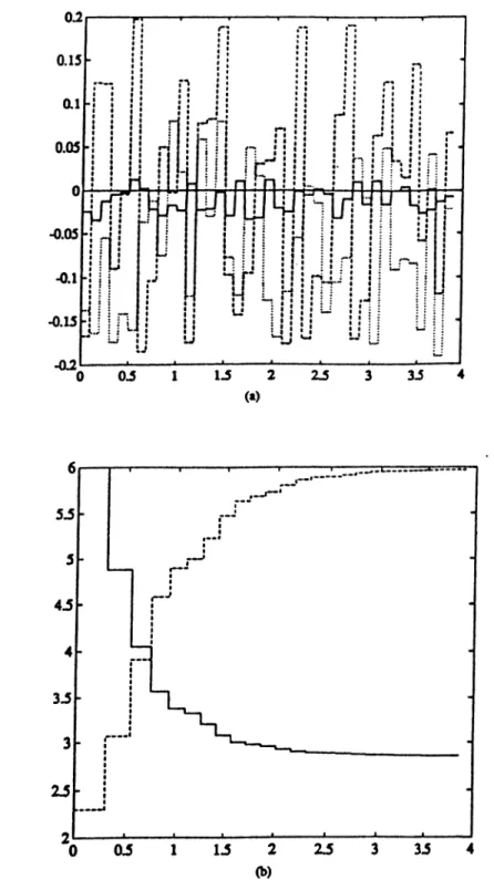
4.2 Simulation results of Example 4 . 1 ... 44

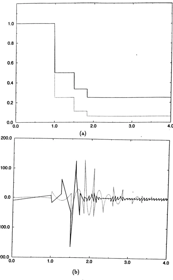
5.1 Simulation results of Example 5 . 1 ... 59

Chapter 1

INTRODUCTION

Robustness problem for sampled-data control systems poses particular challenges. Uncertainties in the continuous-time plant affect both the discrete-time and the inter-sample behavior of the closed-loop control system. Sampling process changes structure information about the perturbations in a complex manner. Choice of the sampling period and hold function are associated problems. Special mathematical tools are required to attack these problems.

Plant uncertainties are modeled as additive perturbations to a completely known nominal system. Various structural conditions can be imposed on perturbations by using physical considerations. In the case of continuous­ time systems robustness performance and its estimates can be improved by using the structure information about the perturbations. For sampled- data control systems, however, structure loss occurs. One approach could be designing a continuous time controller first and then discretizing it at a sufficiently small sampling period, T. Practical considerations, however, forces us to make clear what makes a sampling period “sufficiently small” for the given uncertain system. Instead of using a continuous-time controller design in a sampled-data controller setting, designing the controller with the discretized system in mind provides larger sampling periods. The structure loss of the perturbations can be handled by neglecting discretized uncertainty terms of 0 [ T ‘^) [1]. The remaining terms retain the structure. As T becomes

small, (9(T^) terms become negligible, and the design of the sampled-data controller can be made to depend only on the original continuous-time system’s uncertainty structure.

Uncertainties in the continuous-time description of the continuous­ time system results in exponential-like uncertainties in the closed-loop discrete-time system. Over-bounding the resulting uncertainties as additive perturbations results in too conservative robustness regions. It is possible to improve these bounds by exploiting the exponential uncertainty structure in the sampled-data control system [2]. This analysis must be carried out, however, for every different sampling period that is under consideration. For certain types of parametric uncertainties and sampled-data feedback configurations it is possible to carry out the robustness analysis in the so called “ scaled parameter space” that does not depend explicitly on the chosen sampling period [3]. Approximating the exponential dependence of discrete-time closed-loop response to the uncertain parameter by polynomial rationals is also proposed.

In the design of sampled-data control systems another freedom is the choice o f the sample/hold functions. In [4] it is shown by an example that the use of generalized sample/hold functions can improve the robustness bounds, however, no design methodology is given for achieving robustness. In [5], it is argued against the use of sample hold/functions. Using frequency domain arguments, it is observed that advantages obtained by using generalized sample/hold functions are compensated by poor inter-sample behavior and increased sensitivity to the high frequency characteristics of the original continuous-time plant. The freedom of choice of generalized sample/hold function must be exploited carefully. An overview of these results is given in the next chapter.

For certain classes of uncertain continuous-time systems it is possible to design high-gain type continuous-time controllers which achieve robust stability no matter how large the perturbations are. This approach has been followed in achieving robust stability for various perturbation structures [6], as well as in decentralized stabilization of interconnected systems [8]- [10]. An interesting question is whether robust stabilization is possible using controllers which operate on sampled measurements only. The choice of the

controller structure and the sampling period, and the characterization of stabilizable perturbation structures are some of the accompanying problems.

It is known that when a shift-invariant sampled-data controller is used, then, in general, the system has a finite gain margin that depends on the sampling period, so that one can not use arbitrarily high gains. Although it is possible to achieve arbitrarily large gain margins by using periodically varying feedback gains [11], [12], destabilizing effect of perturbations are also amplified, preventing robust stabilization. A practical solution to the problem has been offered in [4], where it was shown that robustness bounds can be improved using generalized hold functions. However, no class of perturbations for which robust stabilization can be achieved was identified. Obviously, the main difficulty is due to the fact that sampling process changes the structure of the perturbations completely.

In [13] a design methodology for sampled-data counterparts of these “high-gain” controllers is presented. The proposed controllers measure sampled values of the states and apply the control input through generalized sample/holds which simulate continuous-time controllers in the absence of uncertainties. It is shown that robust stability can be achieved when the perturbations satisfy the so called “matching condition” and the sampling period is less than some critical value determined by the size of perturbations.

The outline of the thesis is as follows.

In Chapter 2, an overview of existing results is presented, with emphasis on the design of sampled-data controllers for systems under perturbations.

In Chapter 3 an improved design methodology is presented which guarantees robust stability for a more general time-varying perturbation structure [14]. Effects of additive perturbations in the continuous-time are modeled as multiplicative perturbations to the discrete-time response. This approach enables to use the information on the structure of the perturbation in a direct manner. The controllers that are proposed simulate high-gain continuous time state feedback controllers in the absence of perturbations. Choice o f the sampling period is another interesting problem. The controllers have access to sampled values of the state only, whereas perturbations can

measure the state continuously. Decreasing the sampling period enables the controller to correct the effects of perturbations more often. If the gain is sufficiently high and the sampling period is sufficiently small then the stability of the closed loop system is insensitive to the presence of the perturbations. The same result is also shown to be applicable to decentralized control of interconnected systems.

Based on the result above, in Chapter 4, a similar design methodology is given which enables online adaptation of the controller gains and the sampling period [15]. The proposed controller structure is simplified in order to allow for on line computations.

In Chapter 5 robust adaptive stabilization of systems with more general sector bounded nonlinear time-varying perturbations using sampled-data

output feedback is considered. Restricting the controllers to use output

measurements only makes the problem more complex, since the controllers have the task of estimating the state in a perturbed system in addition to bringing the state to zero. The stabilization method suggested is simple enough to be carried out online, allowing for the controllers to adapt their gains and sampling periods without a priori information on the sizes of the perturbations.

The last chapter is devoted to concluding remarks, and the derivation of various descriptions of systems considered in Chapter 5 are given in the Appendix.

Chapter 2

LITERATURE SURVEY

In [2] Bernstein and Hollot consider the n dimensional, m input q output continuous-time plant

x{t) = (A -f AA)x{t) + {B + AjB)u(í), y{t) = Cx{t) (

2

.

1

)

where A , B , C are real matrices of appropriate dimensions, and A A , A B

represent perturbations in A and B, respectively. Perturbations are assumed to satisfy the structural conditions

A A = Y^ ai Ai, A B = < 1

1=1 *=1 1=1

(

2

.

2

)

where cr,’s are uncertain parameters, and Ai,Bi reflect the structure information. The sarnpled-data controller is assumed to be of the form

u{t) = Ky{mT), mT < t < (m + 1)T' (2.3) where T denotes the sampling period, and K is a constant static gain, which results in the closed loop response

x { { m + l ) T ) = / e(^+^^)"dr(5 + A B )/r C ]x (m r )

Jo

Given arbitrary A A , A B , the system ( 2.4) is discrete-time stable if all the eigenvalues of A B) are included in the open unit disk. Moreover (2.4) is said to be robustly stable if it is discrete-time stable for all Ai4, A B

that satisfy (2.2).

Instead of over-bounding the effect of uncertainties to the discrete-time system as

$t(A A , A B ) = -b

f

e^^drKC] -b A $ (2.5)

Jo

they prefer a more direct approach and look for a discrete-time parameter independent Lyapunov function. Their main result is summarized in the following

T h e o r e m 2.1 If there exists an a > 0 such that

p{M„) < 1 (

2

.

6

)

then the sampled-data control system (

24

) is robustly discrete-time stable,

where and Me =: ( [ / 0] ® [ / 0])eAaT I K C Ae — ■ A B ' 1 A / ■ A B ■ 0 0 + - a l ) e ( 0 0 I

K C

P

+ E

*■=1

Bi

0

0

A.

Bi

0

0

(2.7)

As usual, (g) and 0 denote Kronecker multiplication and addition respectively, and

p{A)

= max{iA,(A)|}

(2.8)

A dual result holds when the input matrix B is certain and there is uncertainty in the output matrix as

The authors leave the problem of checking the existence of a > 0 untouched. Through an example improvement in the robustness bounds is demonstrated.

Dolphus investigates the design of sampled-data controllers for achieving robustness in [1]. The controllers use zero-order-hold and static state feedback. The following m input, uncertain plant is considered.

i { t ) = [A -H A T (r (0 )]a :(0 + [B + ABir{t))]u{t),

(

2

.

10

)

where r(t) denotes possibly time-varying uncertain parameters, and A .4 (r(i))

and AB{ r( t) ) additive perturbations to A and B, respectively. The controller

has the form

u{t) = - F x { m T ) , < t < tm+i, (2-11)

where F is the state feedback gain, tm — mT, and T is the sampling period. Under this feedback the closed-loop control system has the following response

3j[irn+l] ~ ^(^m+1 )

- r)[B -f- A5(r(r))]drF]

where

= [A-l-AT(r(i))]$(i,io)

—

I-The uncertain state transmission matrix is partitioned as 0m = ^0 + Tim

where „

(

2.12)

$0 = i e^^drBF,

Jo

(2.13)

is the nominal discrete-time transition matrix, and T is of order 0 { T) , and it is further decomposed as

r .„ = / ' “ *' [A/l(r(i)) - AB(r(i))i-ldi +

(2.14)

with the remaining term F

2

m being of order O(T^). It can be shown that for stability considerations can be neglected when T is sufficiently small, moreover the 0 { T ) term, Fi^ - F

2

m reflects the original structure of the perturbations. Next, a parameter independent candidate Lyapunov function

Vm = x { t „ , f Px { t m) (2.15)

is chosen, where P is positive definite matrix, which is further used in computing the feedback gain F as

F = { B^PT ^- cRY^B^PA (2.16)

What remains is to choose P and T properly such that the Lyapunov function difference I4i4-i — Kn is a negative-definite function. Finally, the perturbations are assumed to satisfy a so called “rank 1” condition to obtain a sampled-data version of the continuous time method described in [7].

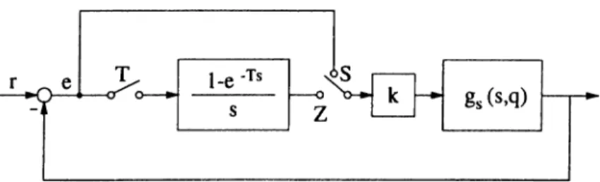
Ackerman and Hu [3] investigate the robustness problem of sampled- data controllers in frequency domain for uncertain physical parameters. They start from a controller structure shown in Fig. 2.1. Related to the robustness problem they search answers to the following questions. For what kind of systems the robustness can be investigated irrespective of the sampling period? For such systems what is the relation between the robustness region of continuous-time controller and the robustness region of the sampled-data controller? Intuitively one expects continuous time- controllers to perform better than sampled-data controllers in robustness. Is this intuition necessarily true? The uncertain physical parameters enter the sampled-data transfer matrix in an exponential form. How could those exponentials be approximated by polynomial rationals?

The following definition is given.

A transfer function Qais^q) with / physical parameters q = [?i,

9 2

? · · · ? qiV is scalable, if there exists a scaled transfer function gv{sT,r)

such that

gs{s,q) = gv{sT,r) (2.17)

where the scaled parameter vector r = r{q, T) is continuous in q and T. As examples, the transfer function = sT{

3

T+qT) scalable, however, the transfer function is not scalable.

The class of scalable transfer functions is quite a large class as indicated by the following lemma.

L e m m a 2.1 The linear ordinary differential equation

'd<‘

n Ji m It' 1=0

(2.18)

in the scalar unknown x(t) with uncertain coefficients a{, bi gives rise to a scalable transfer function.

P r o o f: A new time scaling is achieved by introducing the transformed parameters

ai = aifT\ !3i = bi/T (2.19)

Similar scaling laws can be given for elementary differential equations for electrical circuits and mechanical systems.

T h e o r e m 2.2 I f g,{s.,q) in Fig. 2.1 is scalable, then the stability regions o f continuous and the sampled system can be described in the same space of scaled parameters r o f (2.17).

P r o o f: If g,{s, q) is scalable then we can show that the pulse transfer function

(

2

.

20

)

h^{z,q,T) = ^----^-ZT{gs{s,q)ls]

does not depend explicitly on T. Furthermore, the map defined by u = sT maps left half of the s-plane onto the left half of the u-plane. Therefore, the stability of the continuous-time system can be described isomorphically as a region in the scaled parameter space r. On the other hand, Schur stability of numerator of 1 -f hz{z, r) is naturally described in r. Inserting a discrete-time compensator in to the closed-loop will not change this fact. The compensator transfer function must not be scaled because it describes a relation between input and output sequences independent of the sampling period T.

The stability region in r will be determined by real and complex root boundaries. The authors show that continuous-time real root boundary at 5 = 0 and discrete-time real root boundary at ^ = 1 are identical. Complex root boundaries are in general different.

The authors also provide an example where the inclusion of the zero-order hold in the loop causes an unstable continuous-time system to become stable for a certain range of scaled parameter space.

Finally, the authors note that the terms in the Poisson series expansion

(

2

.

21

)

/i,(e·^) = (1 - e -'^ ) y

sT + ]m2i,/T

converge like ^ as m oo for a strictly proper plant. Thus, the infinite sum in (2.20) may be approximated by a finite sum and the stability region in r

may be approximated by root boundaries of polynomials whose coefficients depend on r in a polynomial rational fashion. It is claimed that information that is necessary for design decisions are contained in the first few terms that are considered.

Most sampled-data controllers are implemented using zero-order hold functions. Kabamba [4] establishes that by using generalized hold functions instead of zero-order hold functions, it is possible to achieve many desirable properties for the associated sampled-data response, including simultaneous pole assignment for several systems, optimal noise rejection and decoupling, arbitrary input/output transfer functions up to the order of the system. Many related results have been studied in the literature. Feuer and Goodwin [5] investigate the robustness problem, when generalized sample- hold function (GSHF) is used. Following the approach in [4], the authors consider the sampled-data control scheme shown in Fig. 2.2, where the continuous-time system is described by the state equations

x{t) = Ax{t) -j- Bu{t)

y{t) = Cx{t).

(

2

.

22

) (2.23)

The controller structure is as depicted in the Fig. 2.2

where T is a predetermined time interval ( sampling period ) and F{t) and

G{t) are periodic functions of period T. The signals y{t) and r{t) are the output and the reference input, respectively, and and r,{t) are their sampled versions.

The sampled state response of the control system can be given as

x ((m + 1)T) = e"^^x{mT) + / (2.25)

Jm T

Using the periodicity of F{t) and G{t) and substituting u{t) from (2.24) gives

where x{i m + 1)T) = + f C ] x { m r ) + gr{mT) T f = [ e^ (^ -^ )5F (r)d r Jo

g = f e^^^~^^BG{T)dT

_Jo (2.26) (2.27)

can be set arbitrarily by proper choice of F{t) and G{t), if (T , B) is controllable. Then, the sampled input/output response becomes

, . I — ^g

- 1 - C(e^^^/ - (2.28)

It is evident that if the system is both controllable and observable, then, provided that pathological values of T are avoided, / and g can be chosen so as to arbitrarily assign the sampled-data closed-loop input/output response function arbitrarily. Note that the solutions for F{t) and G{t) in (2.27) are not unique. This flexibility has been used to achieve multiple objectives such as simultaneous pole assignment for several systems.

There are different approaches for determining F{t) and G{t) in (2.26). Piecewise constant functions, or the minimum power solution

F{t) =

G{t) = 0 < t < T

(2.29) (2.30)

where

are examples.

IV

- i : (2.31)

In order to obtain inter-sample behavior the authors follow a frequency domain approach and arrive at the following result.

Under the conditions given in Fig. 2.2, the frequency content of the continuous-time output, y(t) is given by

where

with

H{w) =

Y{w) = H{w)R3{w)

{a^p +alHs{w))Ho{w - pwo)H{w)

p = —oo (2.32) (2.33) and F { ‘ ) = E p=—OO (2.34) G{t) = £ p— — OO (2.3.5) 2tt W o = Y (2.36) 1 _ Ho{w) = — ---JW (2.37)

Using this result the authors argue that by using generalized hold functions instead of zero-order hold, high frequency components are injected to the system. They provide a bound for the power in the high frequency components in terms of the difference between desired / and that can be achieved by the zero-order hold and a constant gain. They observe that the generalized hold function approach depends upon the generation of high frequency components in the continuous-time output which are then folded when the output is sampled. These folded components are

then superimposed to the base band to give the desired sampled frequency response. High frequency disturbances injected to the system will generate further high frequency components due to the modulation action of the generalized hold function. High frequency unmodeled dynamics may pose serious problems because of the same reason. Finally they provide an example where significant high frequency components are generated in the continuous­ time response, even for a constant set point.

Figure 2.1: Unity-feedback system of Ackermann and Hu

G(t)

IMPULSE TRAIN SAMPUNG

ZERO ORDER HOLD

Chapter 3

ROBUST SAMPLED-DATA CONTROL

USING STATE FEEDBACK

The aim of this chapter is to study robust stabilization of a class of linear systems using sampled-data feedback control. It is shown that a linear, time- invariant system subject to additive perturbations can be stabilized using high-gain periodic feedback from sampled values of the state, provided that the perturbations satisfy certain structural conditions. This result is also extended to decentralized sampled-data control of interconnected systems.

3.1

Single Input Systems

Consider a single-input system S described as

S : x{t) = [A +H{ t ) ] x { t ) + bu{t) (3.1.1)

where x{t) € 7?." is the state and u{t) Ç 7?. is the input of S. A and b are constant matrices of appropriate dimensions, and H{t) represents additive perturbations.

canonical form A = ■ 0 1 ■ 0 ■ 1 , b = 0 . 0 0 .,,. 0 . . 1 . (3.1,2)

where possibly nonzero elements in the last row of A are included in the corresponding row of if(t)· We also assume that H(t) has a lower-triangular structure

ftii(i) 0 ··· 0

h2\{t) h22{i) ··· 0

m

=

(3.1.3)

. ^nl(0 ^n2(0 ■ ■ ■

where hij are unknown, uniformly bounded functions of t with uniformly bounded derivatives of all orders up to n — 1. That is

3 r , i € K · . v i > o

where r/,’ is independent of t. This implies that the open-loop transition matrix + T,t) is uniformly bounded in t and exponentially bounded in T. In the rest of the text the term “bounded” is used in place of uniformly bounded in t] we have abused terminology slightly for the sake of conciseness. We note that the structure of H{t) in (3.1.3) is the most general structure known, which allows stabilizability of S in (3.1.1) by continuous­ time feedback control of the form

Uc(t) = k^x[t) , k G 7?.” (3.1.4)

in the absence of any further information except the boundedness of the perturbations [16].

Our purpose is to stabilize S using a sampled-data feedback of the form

u{t) — k^(t — mT) x { mT) , mT < t < (m + l ) T (3.1.5)

where T is the sampling period to be chosen suitably, and k{·) is a, T-periodic gain. To decide on a reasonable choice of the gain k{·) in (3.1.5), we note

that in the absence of perturbations, the continuous-time feedback control in (3.1.4) has the same effect as the sampled-data control

where

u{t) - — mT) x { mT) , mT < t < { m + l ) T

■ ^,(0 = exp[(A +

(3.1.6)

(3.1.7) Comparing (3.1.5) and (3.1.6), it follows that a reasonable choice for k{·) is

k^{t) = k'^^kit) , 0 < i < T (3.1.8)

and the problem reduces to choosing the constant gain k suitably.

With the control in (3.1.6) applied to <S, the resulting closed-loop system becomes

(3.1.9)

(3.1.10)

S : x{t) = [y4 -|- H(t)]x(t) -|- bk^^k{i — mT) x ( mT) , mT < t < {m + l)T

the solution of which is given by

x(t) = ^ ( t , mT) x { mT) , mT < t < {m + 1)7' where

$ (f,m T ) = $ (i,m T )-f- / ^{t,s)bk^^k{s — mT)ds (3.1.11)

JmT

with $ ( i, s) being the state transition matrix of S. Since $ (i, mT) is bounded for mT < t < {m + 1)T, it follows that S in (3.1.9) is stable if and only if the associated discrete time system

f> : ^(m + 1) = $ r(m )^ (m ) is stable, where we use the notation

$ г ( ” г) = $[(m + 1)T, mT]

for convenience.

(3.1.12)

(3.1.13)

Since the expression in (3.1.11) does not provide sufficient information about how to choose k to make V stable, we seek an alternative expression

for $ to gain more insight into its structure. For this purpose we define the vectors Z i { t ) = b =

[A + H{t)]zi{t)-i,{t) , 1 = 1, 2, . . . , n

and let ^ ( 0 = [ ^n(0 . Z(t) = [ ZnJrl{t) 0

W ith these definitions, we state the following.

M t)

]

0 1

(3.1.14)

(3.1.15)

L e m m a 3.1 The state transition matrix ^( t, mT) in (3.1.11) can be expressed alternatively as é { t , mT ) = ^{ t , mT) W{ mT) + R{t,mT) (3.1.16) where W{ mt) = I — Z{mi) (3.1.17) R{t, mT) = ZU)^k{t — rnT) +

f

^{t, s)Z(s)^k{s — mT)ds JmT

P r o o f. Let i '( i ) denote the right hand side of (3.1.16). Clearly '^{mT) = I. Evaluating the derivative of ^ (i), and noting from (3.1.2), (3.1.14) and (3.1.15) that

Z{t)b = b

Z{t) = [A + H { t ) ] Z { t ) - Z { t ) A - Z { t ) (3.1.18)

we obtain

^{t) = [A + H{t)]<i{t) + bk^^kit - mT) (3.1.19)

Thus 'P(i) satisfies the same differential equation and the initial condition as

^{ t , mT) , and the proof follows.

We note that the decomposition of ^{ t, mT) in (3.1.16) is a general expression independent of the structure of the perturbation matrix H[t).

Evaluating ^{ t, mT) at i = (m + 1)T, we obtain

where ^ ^ (m ) — $[(m + 1)T, mT], ZT{m) = Z{mT), VVV(m) = W{mT) , and

Rrim ) = R[{ni + l)T,mT] (3.1.21)

= Z[{m + l)T]^k{T)

+ / $[(m + 1)T, mT + r ]Z (m T + r ) $ t ( r ) d r

Jo

We now show that the term RT(m) in (3.1.20) can be made arbitrarily small by a suitable choice of the gain k. For this, we denote the bounds on the norms of H{t) and its derivatives as

and state the following.

(3.1.22)

L e m m a 3.2 Let the gain k = k( j ) be chosen such that the eigenvalues of A + bk^ are placed at 'ypi, where pi are arbitrarily fixed, distinct, negative

real numbers, and

7

>

0

fs a parameter. Then, for any e > 0, any T > 0 and

any Bi > 0, / =

0

,

1

, . . . , n —

1

, there exists o

7

* >

0

such that ||i?j(m)|| < e fo r all

7

>

7

* and for all m E Z.^..

P r o o f. With k chosen as in the statement of the lemma, the modal matrix of A + bk'^ is TM where F = d ia g {l,

7

, . . . ,

7

” “ ^}, and

M =

1

^1

1

/^2

L/^r‘

1 (3.1.23)

Thus A + bk^ = rM D M ^ F \ and therefore,

<^k{t) = F M e^ 'A /-^ r-^ (3.1.24)

where D — diag{

7

/i i ,

7

/Z

2

, · · · ,

7

/^n}· Since ||M|| and ||M“ ‘ || are bounded, ||r||

<

7

"·^ and

||r"^|| < 1

for

7

> 1

, and

||e^‘ |l <

where

p. =

m ax{/i/}, it follows from (3.1.24) that for every fixed T > 0

On the other hand, with /r (m ) denoting the integral in (3.1.21), we have

||/r(m)|| <

r \\mm + l)T,mT + T]Z{mT + r)rMe‘^^M-'^r-^\\dT J 0

<

r

||$[(m + l)T ,m T + r]||||Z(m r + T)||||M||||M-'||e^^Mr

»/ 0

< B

t

f

_Jo dr _(3.1.26)

for some Bt > 0 which depends on T, where the identity Z{i)T — Z (t), and the boundedness of $ and Z are used to reach the final inequality. Therefore, for every fixed T > 0, and Bi > 0 ^ / = 0 , 1 , . . . , n — 1

lim II/r(m) II = 0

7—»-oo (3.1.27)

The proof then follows from (3.1.21), (3.1.25), (3.1.26) and boundedness of

Zrim +

1).

The result above implies that, with the gain k chosen as in the statement of Lemma 3.2, the stability of ÔT(ni) is essentially reduced to that of the first term on the right hand side of (3.1.20), which is independent of the gain k. Here comes the structure of the perturbation matrix B (t ) into picture, as we discuss below.

L e m m a 3.3 IVith H{t) having the structure in (3.1.3)and the bounds in

(3.1.22), H r(m ) is a bounded lower triangular matrix with zero diagonal

elements.

P r o o f. From (3.1.2), (3.1.3) and (3.1.14) it follows that z¡{t) has the structure

2,(t) = [0 ··· 0 1 *···*]'^ (3.1.28) where 1 appears in the l*'^ position from the last, and * denotes a bounded function defined in terms of the elements of H{t) and their derivatives. By (3.1.15), Z{t) is a lower triangular matrix with unity diagonal elements, and the proof follows.

T h e o r e m 3.1 Suppose that the perturbation matrix H{t) in (3.1.3) satisfies the bounds in (3.1.22). Then there exists a T* > 0 such that for every 0 < T < T* there exists a sampled-data state-feedback controller of the form

(3.1.6) which stabilizes the system S in (3.1.9).

P r o o f. Consider the discrete-time system T> in (3.1.12), the solution of which satisfies -I- n) = n—1 JJ # (m + /) /=0 ^(rn) , m e 2+ (3.1.29)

where we use the notation n—1

n ^ ( 0 = X {n - l ) X{ n - 2) · · · X (0 ) (3.1.30)

1=0

for a sequence of matrices ( X ( l ) ) . Using (3.1.20), the product in (3.1.29) can be expanded as

n—1 n—1

n ^T(m + 0 = n ^ r (m + /)VUr(m -h /) -l· 'f r( m) (3.1.31)

1=0 1=0 r=I

where ^r(jT^) is a sum of product terms, each of which contains exactly r of the matrices R jim -{■ 1) and n — r of $ j( m -1- l)WT{m -f /).

We now claim that given any pi > 0, there exists a T* > 0 such that n—1

JJ + /)W r(m -f /)|| < Pi 1=0

(3.1.32)

for all 0 < T < T* and m G To prove the claim, we write

$7’ (m)WT(m) = [$T(m ) — IjWrim) -f WT{m) (3.1.33) and expand the product in (3.1.32) a.s

n—1 n—1

$ y (m + /)WT(m + /) = y j[$ x (m ~ f I]Wt{tïi + / ) 4 ~ 0 r ( ^ ^ ) (3.1.34)

where

0

r(jTi) is again a sum of product terms, each containing exactly r of the matrices M^r(m + /) and n — r- of [$ j(m + /) — /]lV r(m + /). Lemma 3.3 implies that

n~l

©n(m) = n + /) =

0

(3.1.35)

1=0

so that the upper limit of the summation in (3.1.34) can be changed to n —

1

. We let

supl|W(t)|| = M,, (3.1.36)

ten

and fix =

( 1

+ —

1

>

0

. Continuity of $ ( t , r ) together with the fact that $ (i, t) = / , implies that there exists

2

"* >

0

such that

||$(i + r , ( ) - / | | < £ * (3.1.37) for all T < T* and t £ TZ. Using (3.1.36), (3.1.37), and the structure of 0 r(m ), we obtain from (3.1.34)

n « T ( m + /)H'T(m + /)| | < ( £ * A /„ ) " + ”f ; ( " ) e ; - ' M ; = p. (3.1.38)

1=0 r = l

for all T < T * and m € .2+, proving the claim. We now fix

0

< r < T*, define

sup ||$(i + r , i)|| = M

4

,

ten (3.1.39)

and for any given > 0, let e, = [p

2

+ - MyjM^ > 0. By Lemma

2

.

2

, the feedback law in (

3

.

1

.

6

)can be designed to have

||i?r(m)|| < tr (3.1.40)

for all m € Using (3.1.39),(3.1.40), and the structure of ^ /(m ), we obtain from (3.1.31)

n

—1

n

«T (m

+

1)11

<

/>. +

E ( ,

(

3

.

1

.

41

)

So far we have shown that given p\,p

2

> 0, there exists a T* >

0

such that with T fixed as 0 < T < T*, and the feedback law designed to satisfy (3.1.40), we have

l k ( m + n)|| < />||^(m)|| , m G 2+

where p — p^-\- p

2

. Letting

^ = sup max {||$(i+ /7’,t)||}

ten o<‘<n-i we have from (3.1.42)

proving the stability of T>, and hence, of S.

(3.1.42)

(3.1.43)

(3.1.44)

The constructive proof of Theorem 3.1 shows that S can actually be made exponentially stable with an arbitrary degree of stability The two components pi and p

2

of p determine the maximum sampling period T*, and the feedback gains for some T < T*. It is clear that to have a larger bound on T one has to choose pi as large as possible. But then p

2

has to be chosen small to keep p <

1

, which in turn requires higher gains as seen from the proof of Lemma 3.2. Thus relative magnitudes of pi and p

2

represent the interplay between the sampling period and the feedback gains.

One drawback of the design procedure in the proof of Theorem 3.1, which originates from the proof of Lemma 3.2 is that the feedback gain ¿(7) depends on the sampling period T. It would be nice if the result of Lemma 2.2 had uniformity in T so that a

70

working for some To < T* would also work for all T < To. This would allow the feedback gain ¿(7) to be designed depending on the upper bound T* only, but independently of the actual value of the sampling period. Although many examples worked out indicated that this is indeed the case, it does not follow readily from the present proof of Lemma 3.2.

3.2 Decentralized Sampled-Data Control

The result of the previous section finds a natural application in decentralized control of interconnected systems, where the interconnections among the subsystems are treated as perturbations on locally controlled decoupled subsystems.

Consider such an interconnected system consisting of N single-input subsystems described as

Si : Xi{t) = A,ic,(i) + hiUi{t) + ^ Hij{t)xj{i) , i e J\f (3.2.1)

is A/·

where Af = {

1

,

2

, . . . , A^}; x ,(i) € 'RA' and u,(i) G R- are the state and the input of Si] Ai and

6

, are constant matrices; and Hij{t) represent the interconnections among the subsystems.

We assume as before that the pairs (/I,,

6

,) are controllable, and in the form given in (

3

.

1

.

2

). To describe the structure of the interconnection matrices Hij{t), we define the structure index of a matrix D = (dij) as

V / I - n i r ii D = 0

(3.2.2) where rrioo is a sufficiently large integer. Thus m{D) indicates the position of a diagonal line parallel to the main diagonal, which borders all nonzero elements of D. We assume that for any index set X C M., the structure indices of Hij[t) satisfy

[m{Hii) - 1] < 0 (3.2.3)

ije i

The reason for assuming this structures for Hij{t) is that they characterize a relatively large class o f interconnections which allow for stabilization with continuous-time decentralized state feedback [16]. Note that for X = {¿}, (3.2.3) requires that m{Hu) < 1, that is, Ha{t) have the structure in (3.1.3).

Imitating the control law in (3.1.6), we apply to Si decentralized sampled- data feedback controls o f the form

where

^ki{t) = exp[(A,· + bikj)t]

Defining = [xjx] u

T

_

- [iz

T T

_{1 ^ 2}

•u

(3.2.5)

4 ' = diag{-4i, ^

2

, . . . , y4jv), K ' and similarly, and H^(t) =

the closed-loop system can be described compactly as

: ¿^ (0 = [A^ + H \ t)]x\ t) + - mT)x^{mT) (3.2.6)

Noting that

= exp{(A^ + (3.2.7)

we observe that of (3.2.6) has essentially the same description as S

of (3.1.9) except the structural constraint on K^. Motivated with this similarity we attempt below to carry over the results of the previous section to stabilization of the interconnected system in (3.2.6). For this purpose, we define $ y (m ) as in(3.1.13), where now

^ \ t,m T ) = ^ \ t , m r ) + f <i>\t,s)B^K ^^l,{s-m T)ds (3.2.8)

JmT

with $^(i, s) being the state transition matrix associated with We also define the matrices Z \ t) and Z^{t) similar to Z{t) and Z{t) of (3.1.15) as follows. With

i j = [ 0 . . . 6 j . . . 0 f (3.2.9) denoting the J**“ column of B , we have

z{(t) =

6

'

= lA‘ + H '{ t ) \ z i ( t ) - z l ( t ) , 1 = 1 , 2 , . ..n i ,j e M ( 3 .2 .W )

from which we construct the matrices

Zi(t) = ( 4 y ( ‘ ) 4 y -i(< ) ■■· ^i

( 0 1

Ziit) =

1

< « ( < )

0

0

) , j € V

and finally the matrices

Z \ t) = [ Z i { t ) Z

2

{t) ■■■ Zi^it)]

Z \ t) =■- [ Z , { t ) Z

2

{t) ··· Zyv(0] (3.2.12)

(3.2.11)

L e m m a 3.4 in (3.2.8) can be expressed as ¥ { t ,m T ) = ^ \ t,m T )W \ m T ) + R \t,m T ) (3.2.13) where W \ m T ) = I - Z \ m T ) (3.2.14) R \ t,m T ) = Z ^ (i)$ ^ (i - m T) + / ^^{t,s)Z\s)^l^{s - rnT)ds JmT

P r o o f. The proof follows exactly the same lines as the proof of Lemma 3.1.

To reproduce the development of Section 3.1, we now cissume that H \ i)

and its derivatives satisfy the bounds in (

3

.

1

.

2 2

) with n replaced by m a x{n ,}, and state the following.

L e m m a 3.5 With the decentralized gains k{ = A;,(

7

) chosen to place eigenvalues of A, + bikj at ■jp] , / =

1

,

2

, . . . , n, ; i € Af, the result of Lemma 2.2 also holds for

i?^(m) = R^[{m + lyr.m T ] (3.2.15)

P r o o f. The proof is similar to the proof of Lemma 3.2 except that matrices A, F, M , etc. are replaced by suitably defined block matrices

etc.

The crucial step in carrying the result of Section

1

to interconnected systems is to obtain a structural condition on VFy(m) = W \m T), similar to one provided by Lemma 3.3, which would imply an identity as in (3.1.35). This is achieved by the following lemma, where for notational convenience we define

m ij(W i) = m{Wij) , i , j e A f (3.2.16)

L e m m a 3.6 With the structure indices of H^{t) satisfying the conditions in (3.S,3), W j(m ) is a bounded matrix whose structure indices satisfy

z <

0

(3.2.17)

for any index set X C A/".

Proof.

We first make the following observations.

1

. As far as the structure indices of W-f(m) are concerned, the derivative terms ¿¡(t) in (3.2.10) are insignificant, and therefore m ,j(W ) would remain the same if the columns of Zf{rn) were defined as

z\{t) = [A-\· H{t)]^b] , / = 0 ,

1

, . . . ,n j - J e A f (3.2.18)

where the superscript / is removed from A and H{t) for convenience.

2. The matrix (A + H f can be expressed as a sum of 2^ product terms as 2 '- 2 { A + H ) ‘ = A '+ X ; A^^ A ^ ^ . . . A ^ ^ (3.2.19) r = 0 where {pip-

2

.. .pr

)2

= r. 3. By simple calculation ■■■ Ajbj bj] = In, (3.2.20)

4. For any partitioned matrix X = {Xij)N,N ,

THijiA^X)

,

mij{XA^) < mij{X) + l , i , j e A f (3.2.21) From the first three observations it follows that the column of the ( i , j ) ‘*' block Wij of W-f(m) is structurally equivalent to

= i E ^ o . . . A^'-W~^’-)ijbj , k < rij

2

2 2

)

where (•),j denotes the block of the indicated matrix. Using the result of the fourth observation, the contribution of w'^ to is bounded by

l</<Tij —k

For every /, 1 < / < —

1

, we have

tI\ I m {W ) - /} _(3.2.23)

1

,

2

, . . . , nj —

1

yields (3.2.24)

- 1 1

r = 0 (3.2.25)

with po = i,pi — j . Suppose for fixed i and j , the maximum in (3.2.24) is achieved at / = /,j, and that in (3.2.25) at {pr — p'J}·, r =

1

,

2

, . . . ,/,j —

1

. Since for any X C Af

'u -i 'u -i U U i * . ) = U U ( K ' ) = I hjEl r

=0

7’=0 (3.2.26) we have S - 1] i,j€l p,q^i (3.2.27) Jel p ^ q ^ f

and the proof follows.

We are now ready to prove a decentralized version of Theorem 3.1.

T h e o r e m 3.2 The result of Theorem 3.1 is also true for the decentrally

controlled sampled-data system in (3.2.6).

P r o o f. The proof follows exactly the same lines as the proof of Theorem 3.1 except that the identity in (3.1.35) has to be shown to hold for some n. For this we choose n = ni + n

2

H--- + wa/^, and note that

for arbitrary matrices A and B. Then referring to (3.1.35), we have

m ,j[

0

;^(m)] = W j{m + /)] n-1

- „ „ [W l{m + n -

1

- r)]} - ((8.-3.2^) Pi.P

2

v,Pn-l€^

with po = f and p„ = j . Since n > N, the sequence of indices (po,Pi, · .. ,Pn) contains at least one cycle. By (3.2.27) each such cycle contributes —1 to the summation. Deleting these cycles leaves a simple path from i to j of length at most —

1

. Thus the right hand side of (3.2.29) can be majorized as

yV

- 2

< „ _ „ m a x _ ^ ^ { ^ m „ ,, ^ J l T ;/ ( m + n - l - r , ) ] } - n (3.2.30) 91i72....,9W-2 _s=0

where are distinct with qo = i, qN-i = i , and the integer

0

< r, < n —

1

depends on which pr qs corresponds to. By definition of structure indices

7 i+ l

SO that

mij[Ql{m)] < ( X ) n ,) - n < -n,· s^i (3.2.31) (3.2.32) (3.2.33) which implies [0n(»Ti)]ij =

0

. Thus

e;(m) = 0

and the proof follows.

Now several remarks are in order.

We first note that the key to our main result is the result of Lemma 3.6, which states that an interconnection structure which satisfies (3.2.3) finally leads to the identity in (3.2.33). Then the question arises: “Can Lemma 3.3 be used to characterize more general interconnection structures for which (3.2.33) is true?” It is strongly believed that any interconnection structure which allows decentralized stabilization by high-gain continuous­ time feedback has this property. But a rigorous proof involves many technical details.

A second remark is concerned with the use of different sampling rates in controlling the subsystems. The composition of in (3.2.13), together with Lemma 3.2, implies that the high-gain sampled-data control in (3.2.4) takes care of the part of the state vector x{m T) in the range

of Z^{mT), leaving an essentially free-running system starting from the

remaining part of the state vector in the range of W^{mT), whose behaviour is independent of the control applied. A closer examination of the control in (3.2.4) reveals that it shows an impulsive behaviour at the sampling instants, and it is precisely this nature of the control that makes the response

to {mT)x{mT) decay rapidly to zero. This observation suggests that

stabilization of the overall system using multirate sampled-data controllers of impulsive nature may also be possible. That this is indeed the case for a special time-invariant interconnection structure has already been proved in [13], but again, a proof for more general interconnection matrices is too detailed and falls beyond the scope of this chapter.

Our final remark, closely related to the previous one, is on the possibility of using alternative, and perhaps, simpler control laws than that considered here. It seems that any control law having a suitable impulsive nature at the sampling instants to cancel the effect of Z \ m T )x{m T ) would work just as well as the control in (3.2.4). This issue is discussed in the next chapter.

Chapter 4

ADAPTIVE ROBUST SAMPLED-DATA

CONTROL USING STATE FEEDBACK

In this chapter robust adaptive sampled-data control of a class of linear systems under structural perturbations is considered. The controller is a time-varying state-feedback law having a fixed structure, containing an adjustable parameter, and operating on sampled values. The sampling period and the controller parameter are adjusted wdth simple adaptation rules. The resulting closed-loop system is shown to be stable for a class of unknown perturbations. The same result is also shown to be applicable to decentralized control of interconnected system.

4.1

Problem Statement and Preliminaries

We consider the single-input system in (3.1.1), whose description we repeat below for convenience

<S: x{t) = [A + H{t)]x{t) + bu{t) (4.1.1)

As in the previous chapter, we assume that the pair {A, b) is controllable and is in the controllable canonical form of (

3

.

1

.

2

) and that H{t) has the lower-triangular form as in (3.1.3).

To the system <S, we apply a sampled-data feedback control of the form

u(i) k {j,

5

*

7

^ ? tjji ^ ¿m

+ 1

(4.1.2)

where tmdenotes the sampling instants, ')rnis a parameter which is constant over each sampling interval but may change from one interval to another, and ¿ ( i ,

7

) is a time-varying feedback gain vector, which is a bounded function of t for every fixed

7

.

Our first objective is to show that the perturbed system in (4.1.1) can be stabilized by a sampled-data controller of the form (4.1.2), and the second objective is to eliminate the need for the information about the bounds of the perturbations.

W ith the control in (4.1.2) applied to S, the resulting closed-loop system becomes

S : x{t) = [A +H{ t ) ] x{ t ) + bk'^{t - tm < t < tm+i (4.1.3)

the solution of which is given by [17]

x (i) ■ ^(^) TiH)^(^m)) ^ t (^’ b4)

where

= ^{ ti t m) + [ T)bk'^ {t - tm ^ m W (4.1.5)

with $ (t,im ) being the state transition matrix of S. Evaluating (4.1.4) at

t = tm+ii we obtain

'D : x{tm+l) — ^(^m+l» T^m)®(^m)

which defines a discrete-time system.

Suppose that the sampling periods, defined as

Tm — tm-\-\

(4.1.6)

(4.1.7) are bounded from above, and that hm,,^—,oo t-m oo. Then, for any t ¿q, there exists an m such that tm < t < tm+i- Since ^ ( i , r ) and k{t,jm) are

bounded for all t and r with tm < r < t < tm+i, it follows from (4.1.4) that

S in (4.1.3) is stable in continuous sense if and only if T> in (

4

.

1

.

6

) is stable in discrete sense. Our immediate purpose is to choose a suitable structure for the gain in (4.1.2) which guarantees stability of T> under certain conditions on

7

m and Tm- For this purpose, we refer to [14], who used a time-varying feedback gain of the form

¿ ^ ( i ,

7

) = /;^(

7

) e x p { [ /H -

6

F (

7

)]i} (4.1.8) where ^^(

7

) is a constant gain which places the eigenvalues of

/ 1

+ bk^{'y)

at —/z

;7

with > 0, / = 1,2, ...,n , being arbitrary distinct numbers. We have already shown in the previous chapter that with the sampling periods

Tm and the parameters

7

^ kept constant as Tm = T and

7

^ =

7

, there exist T* > 0 and

7

* > 0, which depend on the bounds on the perturbations, such that the sampled-data control in (4.1.2) with the gain as in (4.1.8) results in a stable V for all T < T* and

7

>

7

*. We now try to relax the requirement that these bounds be known by adjusting the sampling period Tm and the parameter jm adaptively.

A closer examination of the gain in (4.1.8) reveals that its components behave like Isi,

2

nd, etc. order impulses. Motivated by this observation, we choose the structure of the gain vector k^{t,'y) in (4.1.2) as

(4.1.9) with components

= {

0

! i <

0

' = ·■·’ " ‘ where ¡it >

0

are arbitrary distinct numbers, and the coefficients air are obtained by solving the equations

f^i‘

/^2

‘

- 1

T r - l + l an ■

0

■ —

0

( -

1

)' J (4.1.11)

It is easy to check that ki{t,‘y) behaves like an / —th order impulse for large

7

. That is, linXy_oo

1^00

= /^^” ^^(0) for any function / which is infinitely differentiable at i =

0

.

We next investigate the behavior of the discrete state transition matrix in (4.1.6) for fixed and

7

m. For this purpose, we define as in the previous chapter the vectors

Zi{t) = b,

= [A + H{t)]zi{t) - zi{t), I - 1 ,2 ,...,n,

and form the matrix

Z{t) = [Zn{t) Zn-l{t) ··· Zi(i)].

From (4.1.5), we write

^(i,im ,7m ) = ^t,tra)W{t,ri) + 'i'(<,im,7m) where

W{t) = I - Z{t)

and

and state the following.

(4.1.12)

(4.1.13)

(4.1.14)

(4.1.15)

(4.1.16)

L e m m a 4.1 If H{t) and its derivatives up to order n —

1

ai'e bounded, then

lim ^(t,tm ,'f) =

0

7 —^00

^ (4.1.17)

for all t > t,

P r o o f. Let

We claim that

^ (t,im ,7 ) = ['i'n(<,im,7) ··· ^ l(i,im ,7 )l (4.1.18)

/ /

(4.1.19)

3=1 r = l

/ ^(<,'r)2/+i(7-)e ‘"*^d7

The claim can easily be proved by showing using (4.1.10)-(4.1.12) and (4.1.16) that both sides of (4.1.19) satisfy the same differential equation

i{t) = [A +H{t)]^{t) + b k i{t-t,n ,'r)

(4.1.20) The proof then follows from the boundedness of / = 1 ,2 ,..., n +

1

, which is implied by the boundedness of H{t) and its derivatives.

From (4.1.14) and Lemma 4.1 we observe that with chosen as in (4.1.9)-(4.1.11), and

7

^ sufficiently large, ^(/m+i,/m ,7m ) in (4.1.6) behaves essentially like '5(/m+i, which is independent of

7

m. This observation, together with the structure of W{tm) implied by the structure

of H{t), allows us to reach the following result on the stability of T>.

T h e o r e m 4.1 Let ¿ ^ ( /,

7

) be chosen as in (

4

-

1

.

9

) - (

4

-L ll). Then there exist

r * > 0 ,

7

* > 0 such that T) in (4-1.6) is exponentially stable provided that

7

m < 7*> 0 < Tm < T * , m e Z+.

P r o o f. We first observe that boundedness of H{t) and its derivatives, (4.1.12), (4.1.15), (4.1.16) and Lemma 4.1 imply that

Mu, = sup||lT(/)||

t^n

e(T) = sup sup ||<^(/m+l,/m) -

/11

0

<C.Tm^T

sup sup sup ||i'(im+l,/m,

7

m)|| 7m>7 0<T m <T tmen.

(4.1.21)

all exist, and that

lim e(T) = 0

lim

8

(T,'j) = 0, for all T > 0

||^(/m+l,^m)|| <

1

+ €(T), for all ¿m e 71, T m < T (4.1.22) From (4.1.6) we have n-l 3^(/m4-n) — [JJ ^(/m+/+l>/m+/)7m+/)]^(/m)

1=0

(4.1.23)

Taking the norm of both sides of (4.1.23), expanding the product using (4.1.14), and using (4.1.21) and (4.1.22), we obtain

n - l n

—1

lk(<m«)ll = {ll n

+ E ( ! <lH-<m]'r-'(r,7))||x(i„)||

/=0

/=0

W

(4.1.24)

p r o v id e d T„i < T a n d

7

m >

7

? m € w h ere w e u se th e n o ta tio n

W m + I - W { t n + i ) , = ^ { t m + i + i , t m + i , ^ m + i ) , for C on venience. N o w u sin g th e id e n tity

^m+/W^m+/ = kkm+/ + [^m+i ~ I]^m+l (4.1.25) and (4.1.21), the product term in (4.1.24) can further be bounded as

n

—1

n

—1

/=0

provided Tm < T.

n

< II n ^»"™+<ll +

("')i'(T )

(

4

.

1

.

26

)

/=0

1=0

i=\ W

As can easily be seen from (3.1.3), (4.1.12), and (4.1.15), W{t) is a lower triangular matrix with zero diagonal elements, so that

n

—1

n ^rn+t =

0

(4.1.27)

/=0

(4.1.22), (4.1.26) and (4.1.27) imply that for any pi > 0, there exists a T* > 0 such that

n

—1

n ll«~+l»'m+,||

< / - 1

(4.1.28)

/=0

provided Tm < T * , m e Z+. With T* fixed to satisfy (4.1.28), (4.1.22) and (4.1.24) imply that for any p

2

>

0

, there exists a

7

* >

0

such that

||x(im+n)|| < {pi + P

2

)\\x{tr^ provided Tm <T*,'^m >

7

* ,” ^ ^ -

2

^+· Let p = pi + p

2

< 1- With (4.1.29) r

—1

M = p max II TT ^{tm+l+utm+l,7m+l] l<r<n-l (4.1.30)

we have from (4.1.29)

and the proof follows.

(4.1.31)

We observe from the proof of Theorem 4.1 that for given pi and p

2

i T*

and

7

* depend on the bounds of H {i) and its derivatives, which are unknown. This necessitates the use of an adaptation mechanism to adjust Tm and

7

m based on measurements of x{tm). In the next section we investigate this problem.

4.2

Adaptive Sampled-Data Control

We choose the adaptation rules for the sampling period Tm = im+i — ¿m, and the parameter

7

m in k{t — tm,'ym) of (4.1.2) as

^m+l ~ +<^T||^(^m)

7 m + l = 7 m + <^7|l^(^m)|| (4.2.1)

where

0 7

, To,

7

o > 0 are arbitrary. Thus the closed-loop adaptive control system S in (4.1.3) has the configuration shown in Fig. 4.1.

The system t) in (4.1.6) associated with <S, and the adaptation rules in (4.2.1) define a discrete-time adaptive control system T>a, whose solutions starting from the initial condition XA{to) — (2;o,3o,7o), we denote by ^'/l(^m) Tq, 7o) ~ [^(^m)» Tfn]·

The following theorem states our main result.

T h e o r e m 4.2 Under the feedback control in (4-1.2) with k{t,'f) chosen as

in (4.1.9)-(4-l-ll)y and Tm and -fm adjusted according to (

4

-

2

.

1

), we have

lim Tm m—►oo T o o > 0 , lim Jm = Too >

0

, m

—+00

lim x{tm) =

0

(4.2.2) (4.2.3) (4.2.4)

so that XA{tmi^o,To,^o) is bounded for all To >

0

,to >

0

and x{to) = xq.

P r o o f. Let T* and

7

* be as in the statement of Theorem 4.1. Three cases are possible.

Case I. Trn > T* for all m G Z.^..

In this case, since {Tm} is rionincreasing, Too > T* exists, proving (4.2.2). Then, (4.2.4) follows directly from (4.2.1). (4.2.1) also implies that

m

- 1

r - ' = T„-‘ + ,T T E l W 'i ) l l

/=0

SO that (4.2.5) (4.2.6) 7m = 70 + - To ')

and (

4

.

2

.

3

) follows by taking the limit.

Case II. jm <

7

* for m €

Z^-In this case, the proof follows exactly the same lines as the proof of Case I with the roles of jm and T~^ interchanged.