Modified 3D sensitivity matrix method and use of multichannel current source for magnetic resonance electrical impedance tomography (MREIT)

MODIFIED 3D SENSITIVITY

MATRIX METHOD AND USE OF

MULTICHANNEL CURRENT

SOURCE FOR MAGNETIC

RESONANCE ELECTRICAL

IMPEDANCE TOMOGRAPHY

(MREIT)

A THESIS

SUBMITTED TO THE DEPARTMENT OF ELECTRICAL AND ELECTRONICS ENGINEERING

AND THE GRADUATE SCHOOL OF ENGINEERING AND SCIENCES OF BILKENT UNIVERSITY

IN PARTIAL FULLFILMENT OF THE REQUIREMENTS FOR THE DEGREE OF

MASTER OF SCIENCE

By

Mustafa Rıdvan CANTAġ

January 2012

ii

I certify that I have read this thesis and that in my opinion it is fully adequate, in scope and in quality, as a thesis for the degree of Master of Science.

Prof. Dr. Yusuf Ziya Ġder (Supervisor)

I certify that I have read this thesis and that in my opinion it is fully adequate, in scope and in quality, as a thesis for the degree of Master of Science.

Prof. Dr. Ergin Atalar

I certify that I have read this thesis and that in my opinion it is fully adequate, in scope and in quality, as a thesis for the degree of Master of Science.

Prof. Dr. Murat Eyuboğlu

Approved for the Graduate School of Engineering and Sciences:

Prof. Dr. Levent Onural

iii

ABSTRACT

MODIFIED 3D SENSITIVITY MATRIX

METHOD AND USE OF

MULTICHANNEL CURRENT SOURCE

FOR MAGNETIC RESONANCE

ELECTRICAL IMPEDANCE

TOMOGRAPHY (MREIT)

Mustafa Rıdvan CANTAġ

M.S. in Electrical and Electronics Engineering

Supervisor: Prof. Dr.Yusuf Ziya Ġder

January 2012

Magnetic Resonance Electrical Impedance Tomography (MREIT) is a technique to image the electrical conductivity distribution inside the object (such as a human body). This technique consists of three steps: current injection into the object, the measurement of the magnetic flux density by a Magnetic Resonance Imaging (MRI) system, and the reconstruction of the conductivity distribution from the measured magnetic flux density. Although there are other algorithms to reconstruct the conductivity distribution inside the object, in this thesis, the Sensitivity Matrix Method is investigated for 3D problems. In MREIT, the use of the Sensitivity Matrix Method is not common for 3D problems. This is because of the fact that for 3D problems the Sensitivity Matrix Method requires large memory space and long calculation time. Calculation of the sensitivity matrix is the most time consuming part of this method. Therefore in this thesis, a modification is proposed in order to reduce the calculation time of the sensitivity matrix. Since the sensitivity matrix will be calculated at each iteration, this modification speeds up the algorithm significantly. Also by making several assumptions regarding the conductivity distribution of the object, the problem may be further reduced. In this thesis, conductivity distribution inside the object

iv

is assumed to be z-invariant (z is the direction of the main magnetic field of the MRI system).Thus the dimension of the sensitivity matrix and the time required to calculate the conductivity distribution inside the object significantly decrease. Another problem with the application of the Sensitivity Matrix Method is that the magnetic flux density calculated by subtracting the calculated magnetic flux density (for the assumed initial conductivity distribution) from the measured one has errors. These erros are results of the boundary mismatches between the simulation object and the real object, inaccuracies in calculations and measurement artifacts. In this thesis, use of a multichannel current source is proposed in order to reduce these errors. Using the multichannel current source not only reduces the errors due to the boundary mismatches and other reasons but also sustains a nearly uniform current distribution inside the object.

Keywords: Magnetic Resonance Electrical Impedance Tomography (MREIT),

Magnetic Resonance Imaging (MRI), Multichannel Current Source, Sensitivity Matrix Method (SMM) , Modified Sensitivity Matrix Method (MSMM)

v

ÖZET

DEĞĠġTĠRĠLMĠġ 3B HASSASĠYET MATRĠSĠ METODU

VE ÇOK KANALLI AKIM KAYNAĞININ MANYETĠK

REZONANS ELEKTRĠKSEL EMPEDANS TOMOGRAFĠ

(MREET) ĠÇĠN KULLANILMASI

Msutafa Rıdvan CANTAġ

Elektrik ve Elektronik Mühendisliği Bölümü Yüksek Lisans Tez Yöneticisi: Prof. Dr. Yusuf Ziya Ġder

Ocak 2012

Manyetik Rezonans Elektriksel Empedans Tomografi (MREET) bir cism (örneğin insan vücudu) içerisindeki elektriksel iletkenlik dağılımını görüntülemek için kullanılan bir yöntemdir. Bu yöntem üç aĢamadan oluĢmaktadır: cisime akım uygulanması, manyetik akı yoğunluğunun Manyetik Rezonans Görüntüleme sistemi ile ölçülmesi ve ölçülen manyetik akı yoğunluğundan iletkenlik dağılımının oluĢturulması. Her ne kadar, cisimin elektriksel iletkenlik dağılımını oluĢturmak için baĢka algoritmalar olsa da bu tezde Hassasiyet Matrisi Metodu üç boyutlu (3B) problemler için incelenecektir. Hassasiyet Matrisi Metodu, MREET'de 3B problemler için yaygın olarak kullanılan bir yöntem değildir çünkü Hassasiyet Matrisi Metodu'nun üç boyutlu problemlerde uygulanması için gereken bilgisayar hafızası ve zaman oldukça fazladır. Hassasiyet matrisinin hesaplanması, bu yöntemin en çok zaman alan kısmıdır. Dolayısıyla bu tezde hassasiyet matrisinin hesaplanma süresini düĢüren bir değiĢiklik önerilmiĢtir. Hassasiyet matrisi her yenileme basamağında hesaplandığı için, bu değiĢiklik algoritmayı önemli ölçüde hızlandıracaktır. Ayrıca iletkenlik dağılımı için varsayımlar yapılarak çözümü kolaylaĢtırmak mümkündür. Bu tezde cisimin içerisindeki iletkenlik dağılımının z den (z MRG sisteminin ana manyetik alan yönüdür) bağımsız olduğu kabul edilmiĢtir.

vi

Böylece hassasiyet matrisinin boyutu küçülmekte ve cisim içerindeki iletkenlik dağılımının hesaplanması için gereken süre önemli ölçüde azalmaktadır. Hassasiyet Matrisi Metodu'nun uygulanmasında karĢılaĢılan bir baĢka problem ise varsayılan ilk iletkenlik değeri için hesaplanan manyetik akı yoğunluğu, ölçülen manyetik akı yoğunluğundan çıkartıldığında, elde edilen manyetik akı yoğunlunda hataların olmasıdır. Bu hatalar simülasyonda kullanılan cisimle gerçekte kullanılan cismin kenar bilgilerinin örtüĢmemesinden, simülasyonda

yapılan hesaplardaki hatalardan ya da ölçümlerdeki yanlıĢlardan

kaynaklanabilmektedir. Bu tezde, bu hataları azaltmak için çok kanallı akım kaynağının kullanılması önerilmiĢtir. Çok kanallı akım kaynağı bu hataları azaltmakla kalmayıp cisim içerisinde neredeyse homojen bir akım dağılımı sağlamaktadır.

Anahtar Kelimeler: Manyetik Rezonans Elektriksel Empedans Tomografi (MREET), Manyetik Rezonans Görüntüleme (MRG), Çok Kanallı Akım Kaynağı, Hassasiyet Matrisi Metodu (HMM), DeğiĢtirilmiĢ Hassasiyet Matrisi Metodu (DHMM)

vii

Acknowledgements

I would like to thank the people who made this thesis possible.

In the first place, it is my pleasure to express my thanks to Prof. Dr. Yusuf Ziya Ider for his invaluable guidance and support throughout my studies. I would also like to thank Prof. Dr. Ergin Atalar and Prof. Dr. Murat Eyüboğlu for accepting to be a member of my thesis jury. My parents Ceylan and Sultan CantaĢ, and my siblings Gökhan and Meltem deserve special mention for their support and encouragement. I also want to thank my colleagues and friends Necip Gürler, Fatih Hafalır, Merve Begüm Terzi, and HaĢim Meriç for giving me pleasant time when working with them. My special thanks are owed to Ömer Faruk Oran for his support and friendship. Finally, I wish to thank my girlfriend Nermin Kondakçı for her support and patience.

viii

Table of Contents

1. ACKNOWLEDGEMENTS ... VII

2. CHAPTER 1 : INTRODUCTION ... 1

1.1OBJECTIVE AND SCOPE OF THE THESIS ... 3

1.2OUTLINE OF THE THESIS ... 5

3. CHAPTER 2 : MODIFIED 3D SENSITIVITY MATRIX METHOD ... 6

2.1CONVENTIONAL SENSITIVITY MATRIX METHOD ... 6

2.1.1FORWARD AND INVERSE PROBLEMS ... 6

2.1.2ALGORITHM OF CONVENTIONAL SENSITIVITY MATRIX METHOD ... 11

2.2MODIFIED SENSITIVITY MATRIX METHOD ... 11

2.2.1ALGORITHM OF MODIFIED SENSITIVITY MATRIX METHOD ... 12

2.3SIMULATION RESULTS ... 12

2.3.1SENSITIVITY ANALYSIS IN Z-DIRECTION ... 14

2.3.2COMPARISON OF THE CONVENTIONAL SENSITIVITY MATRIX METHOD WITH THE MODIFIED SENSITIVITY MATRIX METHOD ... 16

4. CHAPTER 3 : MULTICHANNEL CURRENT SOURCE FOR MREIT ... 19

3.1EFFECTS OF ERRORS IN BOUNDARY AND ELECTRODE POSITIONS TO THE DIFFERENCE MAGNETIC FIELD ΔB_z ... 19

3.2KNOWN PROBLEMS WITH SINGLE CHANNEL CURRENT SOURCE IN MREIT ... 22

3.3USING MULTICHANNEL CURRENT SOURCE IN MREIT ... 24

3.4EXPERIMENT: INVESTIGATION OF THE EFFECT OF THE MULTI CHANNEL CURRENT SOURCE ON ΔB_z ... 25

3.4.1ACQUISITION OF THE Z COMPONENT OF THE MAGNETIC FLUX DENSITY (B_z) ... 25

3.4.2EXPERIMENTAL PROCEDURE AND RESULTS ... 26

5. CHAPTER 4 : SIMULATION AND EXPERIMENTAL RESULTS FOR CONDUCTIVITY RECONSTRUCTION ... 31

4.1SIMULATION RESULTS OF CONDUCTIVITY RECONSTRUCTION FOR 3D OBJECT ... 31

4.2SIMULATIONS FOR MULTICHANNEL CURRENT SOURCE WITH CUBIC PHANTOM ... 35

4.3EXPERIMENT 1:MREIT EXPERIMENT FOR AN INSULATING OBJECT USING MULTICHANNEL CURRENT SOURCE ... 42

4.4 EXPERIMENT 2:MREIT EXPERIMENT FOR AN AGAR OBJECT USING MULTICHANNEL CURRENT SOURCE ... 45

6. CHAPTER 5 : CONCLUSIONS AND DISCUSSIONS ... 52

7. APPENDIX A ... 58

DERIVATION OF THE ΔDσ₀TERM ... 58

8. APPENDIX B ... 59

ix

List of Figures

Figure 2.1 (a) 3D object (b) 3D mesh of the object with tetrahedron finite elements ... 7 Figure 2.2 a) Cylindrical simulation phantom b) Mesh of the cylindrical

simulation phantom ... 13 Figure 2.3 a) Position of the objects placed in to the phantom simulation

phantom b)The real conductivity distribution at the center slice of the phantom ... 13 Figure 2.4 The sensitivity of the center slice magnetic field to an element which is located in the center slice is given ... 14 Figure 2.5 Distance of the element to the center slice of the phantom (slice)

versus the maximum absolute sensitivity value of the center slice magnetic field to the element. ... 15 Figure 2.6 Conductivity distributions acquired using the Conventional

Sensitivity Matrix Method for the three iteration ... 16 Figure 2.7 Convergence of the conductivity distribution and magnetic field

versus iteration number for the conventional sensitivity matrix method ... 16 Figure 2.8 Conductivity distributions acquired using the Modified Sensitivity

Matrix Method for the three iterations (1,3 and 5. iterations) ... 17 Figure 2.9 Convergence of the conductivity distribution and magnetic field

versus iteration number for the modified sensitivity matrix method ... 17 Figure 3.1 a) Simulation phantom with recess electrode parts b) Center slice of

the simulation phantom c) Selected recess part of the phantom ... 20 Figure 3.2 "1 mm" shift of the selected recess part towards to +y direction ... 21 Figure 3.3 Spin echo pulse sequence and current injections for positive and

negative directions. ... 26 Figure 3.4 Cubic phantom with multiple electrodes ... 26 Figure 3.5 Conductivity distribution inside the phantom on the MRI magnitude

image ... 28 Figure 3.6 Electrodes used to inject current into the object and imaging slice

(Top Left) The magnetic flux density difference acquired for the six electrode current injection profile. (Bottom Left) The magnetic flux density measured for the six electrode current injection profile (Top Right) The magnetic flux density calculated for the six electrode current injection profile and uniform conductivity distribution (Bottom Right) ... 29 Figure 3.7 Electrodes used to inject current into the object and imaging slice

(Top Left) The magnetic flux density difference acquired for the multiple (30) electrode current injection profile. (Bottom Left) The magnetic flux density measured for the multiple (30) electrode current injection profile (Top Right) The magnetic flux density calculated for the multiple (30) electrode current injection profile and uniform conductivity distribution (Bottom Right) ... 30 Figure 4.1 a) Simulation phantom b) z-y cross section of the phantom ... 31

x

Figure 4.2 z-y cross section of the simulation phantom, the slices where the Bz's

are calculated and the boundaries of the regions where the conductivity

distribution is z invariant. ... 32

Figure 4.3 Reconstructed conductivity distribution for the first case ... 33

Figure 4.4 Reconstructed conductivity distribution for the second case ... 34

Figure 4.5 Reconstructed conductivity distribution for the third case ... 34

Figure 4.6 a) Simulation phantom b) Real conductivity distribution at the center slice of simulation phantom ... 35

Figure 4.7 a) Magnetic flux density for the first current injection direction and the real conductivity distribution b) Magnetic flux density for the second current injection direction and the real conductivity distribution ... 36

Figure 4.8 a) Magnetic flux density for the first current injection direction and the uniform conductivity distribution b) Magnetic flux density for the second current injection direction and the uniform conductivity distribution ... 36

Figure 4.9 a) Difference magnetic flux density for the first current injection direction b) Difference magnetic flux density for the second current injection direction ... 37

Figure 4.10 a) Conductivity distribution acquired from the ΔB 's by SVD with _z tolerance 0.01 b) Filtered conductivity distribution acquired from the z ΔB 's by SVD with tolerance 0.01 ... 38

Figure 4.11 a) Conductivity distribution acquired from the ΔB 's and the exact _z D matrix by SVD without any truncation. b) Conductivity distribution acquired from the ΔB 's and the exact D matrix by SVD with _z tolerance=0.01 c) Conductivity distribution acquired from the ΔB 's and _z the exact D matrix by SVD with tolerance=0.001 ... 39

Figure 4.12 2D mesh which is used to construct 3D mesh by extrusion ... 40

Figure 4.13 Refined 2D mesh which is used to construct 3D mesh by extrusion ... 40

Figure 4.14 a) Conductivity distribution acquired using the refined mesh from the ΔB 's by SVD with tolerance 0.01 b) Filtered conductivity _z distribution acquired using the refined mesh from the ΔB 's by SVD _z with tolerance 0.01 ... 41

Figure 4.15 z-y cross section of the phantom and the positions of the additional electrodes ... 41 Figure 4.16 a) Conductivity distribution acquired using the refined mesh and

the extra electrodes, from the ΔB 's by SVD with tolerance 0.01 b) _z

Filtered conductivity distribution acquired using the refined mesh and the

extra electrodes, from the ΔB 's by SVD with tolerance 0.01 ... 42_z

Figure 4.17 Cubic phantom with multiple electrodes and the object position inside the phantom (Top Left) outside view of the phantom and the placement direction of the phantom into the MRI scanner (Bottom Left) placement of the object into the phantom with background solution (Top

xi

Right) MR magnitude image of the center slice of the phantom (Bottom

Right) ... 43

Figure 4.18 Current injection directions ... 44

Figure 4.19 a) The difference magnetic flux density acquired for the first current injection direction b) The difference magnetic flux density acquired for the first current injection direction ... 44

Figure 4.20 Acquired conductivity distribution for the multichannel current source experiment with a balloon object ... 45

Figure 4.21 a) Phantom for experiment b) Experiment setup for MREIT ... 46

Figure 4.22 a) Position of the object in phantom which is prepared for experiment b) z-y cross section of the phantom. ... 46

Figure 4.23 z-y cross section of the experiment phantom, the slices where the Bz's are measured and the boundaries of the regions where the conductivity distribution is z invariant. ... 47

Figure 4.24 Reconstructed conductivity distribution for the first case ... 48

Figure 4.25 Reconstructed conductivity distribution for the second case ... 48

Figure 4.26 Reconstructed conductivity distribution for the third case ... 48

Figure 4.27 ΔBz distributions for two current injection directions at 13 slices. (1. slice is the bottom and 13. slice is the top slice of the phantom)( ΔBz 's which are related to the 1. current injection direction are given at left side of each line. ΔBz 's acquired from the 2. current injection directions are shown at the right side of the each line.) ... 51

Figure 5.1 Maximum absolute sensitivity values of the center slice magnetic flux density to the change in the conductivities of each element in conventional sensitivity matrix (sensitivity map which is acquired from conventional sensitivity matrix ). ... 53

Figure 5.2 Maximum absolute sensitivity values of the center slice magnetic flux density to the change in the conductivities of each element in modified sensitivity matrix (sensitivity map which is acquired from modified sensitivity matrix ). ... 54

Figure 5.3 Ratio of the sensitivity maps, which is calculated element by element. ... 54

Figure B. 1 (a) MRI magnitude image (b) boundary acquired from the Sobel edge detection algorithm ... 59

Figure B. 2 MRI magnitude image ... 60

Figure B. 3 (a) Sampling points chosen on the MRI magnitude image and the constructed boundary (b) 2d mesh produced for the constructed boundary information ... 60

xii

List of Tables

1

Chapter 1 : Introduction

Magnetic Resonance Electrical Impedance Tomography (MREIT) is a technique to image electrical conductivity distribution inside the object. In medical imaging, human body is used as an object to be imaged. Since the electrical conductivity of the different cells and the tissues of the body have different electrical conductivity, this method can be used as an another contrast in the MRI system. Also some of the cancerous tissues can have different conductivity values than the healthy ones [1]-[3]. Therefore, the use of MREIT might be a helpful tool in the detection of the cancerous tissues in the body.

In MREIT it is necessary to inject current into the object. Current injection is made into the object by surface electrodes placed over the object. The injected current into the body, creates a magnetic flux around it. If the z is the direction of the main magnetic field of the MRI system, the z component of the magnetic flux

density (B ) inside the object can be measured by the Magnetic Resonance _z

Imaging (MRI) System. After acquiring the B distribution, the conductivity _z

distribution of the object can be reconstructed from this B distribution. There are _z

several algorithms to reconstruct conductivity distribution of the object from the

measured B . The Sensitivity Matrix Method which is discussed in this thesis, is z

one of them.

The relation between the magnetic flux density generated by the internal current distribution and the conductivity of an element is nonlinear. Therefore, in order to easily calculate the conductivity distribution from the magnetic flux density measurements, it is necessary to linearize the forward problem. Here the forward problem is defined as the calculation of the magnetic flux density which is produced by the internal current density of the object. If the forward problem is linearized around an initial conductivity distribution, the relation between the

2

magnetic flux density and the conductivity will be B = D σ σ (usually a _z ( )

uniform conductivity distribution is chosen as an initial conductivity distribution). If the forward problem is solved with the Finite Element Method

(FEM), then the object is divided into N finite element. For M B measurement _z

points the size of theD matrix will be MxN. Here the D matrix is called as the

sensitivity matrix.

In 1998 the sensitivity matrix method is applied to MREIT by Ider and Birgul [4] for 2D problems. Also this method is applied for the 3D problems by Birgul at al [5]. In this work the conductivity distribution of the 3D object is calculated

from the multi slice B measurements, at 5 different slices. However, _z

constructing sensitivity matrix for 3D problems requires very long time and large memory in the computer. This is why the Sensitivity Matrix Method is not commonly used for 3D problems.

In order to improve the performance of the Sensitivity Matrix Method for 3D problems a method is suggested by Hamamura [6]. This method, assumes that the electrodes are placed on the whole length of the object in z direction and the

conductivity distribution of the 3D object is z- invariant. Let's define Bz_ 2D as

the magnetic flux density distribution for a 2D object, and Bz_ 3D as the

magnetic flux density distribution which is calculated at the center slice of a 3D object. Let's assume that the conductivity distribution of the 3D object in x-y plane is equal to the conductivity distribution of the 2D object which lies in x-y plane and the conductivity distribution of the 3D object is z invariant. In this

case, it is claimed that by using a Z correction factor, Bz_ 2D can be transferred

to the Bz_ 3D. Conversely, the Bz_ 3D can also be transformed to the Bz_ 2D using

the Z correction factor. Therefore, if a B_{z_ 3D} measurement is made at the center

slice of the 3D object, this magnetic flux density can be converted to the B_{z_ 2D}

3

object. Since B_{z_ 2D} and B_{z_ 3D} distributions can be converted to the each other

by a Z correction factor, after measurement of the magnetic flux density from the 3D object, whole problem can be solved in 2D. This method reduces the time required to solve the conductivity distribution in an object. However, it is based on the assumption that the conductivity of the object is z invariant and the electrodes should run the whole length of the object . In practice, even the conductivity distribution inside an object is z invariant, using such a long electrode is impractical.

The performance of the MREIT algorithms also depends on the current density distribution inside the object. It is known that uniform internal current density distribution is desirable in order to obtain less noisy images. Song at al [7] designed a new electrode such that the uniform current distribution is achieved under the electrode surface. In this design, the thickness of the electrode is varying over the electrode in order to sustain a uniform current distribution under the surface of the electrode. The design is based on the assumption that conductivity distribution under the surface of the electrode is uniform. However, conductivity distribution may vary under the surface of the electrodes. In these cases the uniform conductivity distribution may not be achieved.

1.1 Objective and Scope of the Thesis

In Magnetic Resonance Electrical Impedance Tomography (MREIT), there are many algorithms to reconstruct conductivity distribution inside the object. One of these algorithms is the Sensitivity Matrix Method. However, this algorithm is not commonly used in 3D problems due to the fact that this method requires too much memory and time. Objective of this thesis is to investigate these limitations and bring solutions to them so that this algorithm can be used for solving 3D problems effectively.

The main limitation of this algorithm for 3D problems is that the construction of

4

sensitivity matrix D is too large. Due to the size of the D matrix, this algorithm

necessitates large memory space. In this thesis, the object is divided into N finite

element to solve the forward problem, and the calculation of the D matrix is

made by changing each elements' conductivity to observe the change in the magnetic flux density at M measurement points. Therefore, the number of the

required forward problem solution in order to construct the D matrix is equal to

the number of the finite elements used to discretisize the object. Since there are

many finite elements in a 3D object, the required calculations for the D matrix is

time consuming. In this thesis, the calculation of the D matrix is simplified to

decrease the time required to construct it. New calculated D matrix is called as

the modified sensitivity matrix. Although the modified sensitivity matrix D is a

modified version of the real one, conductivity distributions solved iteratively using these matrices, converge almost the same solution.

Another limitation of using a D matrix with a large size is that solving

z

ΔB = DΔσ for Δσ requires too much memory and time. In this thesis, an

assumption is made for the elements of the Δσ vector, which results in reduction

in the dimension of Δσ vector and so in the dimension of the D matrix. This

reduction in the dimension of the D matrix not only reduces the memory space

required to save D matrix but also results in reduction in the time required to

solve ΔB = DΔσ equation for reduced _z Δσ vector.

In the Sensitivity Matrix Method, it is necessary to calculate B (the z _z

component of magnetic flux density) for a uniform conductivity distribution of

the object. B is calculated for a uniform conductivity case at the measurement _z

points of B measured by MRI. The difference between the calculated and _z

measured B , gives _z ΔB which is the magnetic flux density arising from the _z

difference of the conductivity of the object from the uniform conductivity. However, due to the fact that the model of the object cannot be constructed with

5

faulty. Also, inaccuracies in calculations and artifacts in measurements creates

errors in ΔB . All of the errors mentioned above are dominant in the regions _z

where the magnetic flux density changes rapidly. In this thesis, it is proposed that using a multichannel current source reduces these errors by producing uniform current distribution inside the object.

1.2 Outline of the Thesis

This thesis consists of five chapters. The second chapter discusses the Modified Sensitivity Matrix Method by comparing it with the Conventional Sensitivity Matrix Method. Boundary mismatches between the simulation object and the

real object create errors on ΔB . In the third chapter, errors in _z ΔB are _z

investigated for different boundary mismatch cases. Then, in this chapter the use of the multichannel current source for the MREIT is discussed. The simulation and experimental methods and the results obtained by using these methods are given in each chapter to clarify the methods. Simulations and experiments based on the results of previous chapters are also given in the forth chapter. Finally, in the fifth chapter conclusions of the thesis are given.

6

Chapter 2 : Modified 3D Sensitivity

Matrix Method

The Sensitivity Matrix Method is an algorithm to reconstruct the conductivity distribution inside the object. This method has usually been used for 2D problems. This is because of the fact that the calculation of the sensitivity matrix requires too much time. Also in 3D case the size of the sensitivity matrix becomes too large which may cause too long solution time and memory problem. The Modified 3D Sensitivity Matrix Method is developed in order to reduce the construction time of the sensitivity matrix, based on the Bz-Substitution MREIT algorithm suggested by Ider [8]. While Bz-Substitution MREIT was proposed for 2D problems, Modified 3D Sensitivity Matrix Method is proposed for 3D problems. Actually, both of these methods can be seen as a modified form of the Conventional Sensitivity Matrix Method. So, this chapter starts with explaining the algorithm of the Conventional Sensitivity Matrix Method and its disadvantages. After that, the advantages which come with the Modified Sensitivity Matrix Method, will be explained.

2.1 Conventional Sensitivity Matrix Method

After acquiring magnetic flux density data using a MRI system we need to reconstruct the conductivity of the object that we want to image. There are several conductivity reconstruction algorithms and one of them is the Conventional Sensitivity Matrix Method. This algorithm is an iterative algorithm to reconstruct electrical conductivity of an object from z component of the measured magnetic flux density. Algorithm consists of two main parts as forward and inverse problems.

2.1.1 Forward and Inverse Problems

Aim of the forward problem is to calculate the magnetic field produced by internal current distribution for known boundary and conductivity distribution.

7

On the other hand, calculation of conductivity distribution inside the object from the measured magnetic field is called inverse problem.

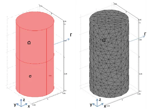
For solving the forward problem, the Finite Element Method can be used. For 3D case if we have a connected and bounded domain Ω in the xyz plane which is shown in Figure 2.1-a, with boundary Г, unit outward normal along Г, n, and positive non-zero conductivity σ, then potential field Φ in Ω should obey the

Laplace's equation   .( ) 0 in Ω. Also defining Neumann boundary

condition J_app

n    

 on Г, where Japp represents the injection pattern, we can

solve Φ using FEM. Integral of Japp on Г should be zero for the considered

injection pattern.

a b

Figure 2.1 (a) 3D object (b) 3D mesh of the object with tetrahedron finite elements

FEM necessitates to divide domain Ω into small finite elements, in order to solve potential field Φ. An example of mesh generated by dividing domain Ω into

8

N=34892 tetrahedron finite elements with n=6974 nodes given in Figure 2.1-b. If we use linear shape functions for finite elements and take conductivity constant

inside each finite element we will have a conductivity value vector σ=[ σ1, σ2, . .

., σN ]' which has dimension Nx1 (34892x1). Using linear finite elements, FEM

calculates the node potentials at the nodes of these finite elements. Because of the fact that we use linear shape functions for the finite elements, potential field at any point is assumed to vary linearly within each element. Thus potential field at any space point can be expressed as a linear combination of node potentials. Using boundary conditions and linear equations for each element, it is possible to write following equation:

( ) 

A Φ b

Here A( ) is n by n coefficient matrix which is acquired from geometry and the

conductivity distribution of the object, Φ is a n by 1 vector which represents the

unknown node potentials, and b is n by 1vector defining the boundary conditions

on the nodes. Solving A( ) Φ b equation for Φ we can obtain potential values

for each node. Using the equations E Φ and J = σE it is possible calculate

electric field and current density for each finite element. Since potential field linearly varies in each element, electric field and current density will be constant inside each element.

In order to calculate magnetic flux density Savart Law will be used. Biot-Savart Law relates the magnetic flux density to the current density as:

0 ( ') ( ', ') ( ') ( ', ') ' ' ' 3 2 2 _{2 2} ( ') ( ') ( ') ( , , ) 4 y y J_x x y x x J_y x y B dx dy dz x x y y z z x y z z





Since the current density is constant inside each finite element, it is possible to discretize this equation. Magnetic flux density of the jth node

j

z

B at ( ,x y z_{j j}, _j) .

will be the sum of the magnetic flux densities at the jth node which are produced

from the current densities of each element with center points ( ,x y z and _{i i}, )_i

9 0 ( ) ( , ) ( ) ( , ) 3 1 2 2 _{2 2} ( ) ( ) ( ) 4 N y_j y J_{i x} x y_{i i} x_j x J_{i y} x y_{i i} B V j i i x_j x_i y_j y_i z_j z_i z



Actually, by solving forward problem we want to calculate measured magnetic flux density by MRI. If we have acquired our MRI image at M nodes, our

measured B vector will have a size Mx1, So the calculated _z B will also have _z

Mx1 size. In order to calculate this B vector we can write a vector equation in z

the following form, using equation which is written for j z B :  z x x y y B C J + C J

where C C are M x N matrices which depend only on the geometry and which _x, _y

are obtained from the discretized Biot Swart Law, and J J_x, _y are Nx1 vectors

containing the x and y components of current densitiy of each finite element. Since the current density of each element is equal to the electric field of that

element times the conductivity of that element (J i_x( )E i_x( ) ( ) i and

( ) ( ) ( )

y y

J i E i  i ) , we can write J = S σ and _{x x} J = S σ_{y y} , by placing each of the

electric field value of the i'th element to the i'th diagonal entry of N x N S matrix (S (i, i) = E (i) and _{x x} S (i, i) = E (i)_{y y} ). So B can be written in the following _z

form:

z x x y y

B = C S σ + C S σ

If we take this equation into the σ parenthesize and call D inside the parenthesize

(B = C S + C S σ_z ( _{x x y y}) ) we will have an equation which is given below.

z

B = Dσ

In the conventional sensitivity matrix method as an inverse problem we have to

find conductivity distribution σ from measured B according to the equation _z

above. In this equation the only known is measured B . Since _z D is a function of

σ and it is desired to find σ , an iterative solution can be used for finding σ . The

10

consists of an initial conductivity value for each finite element. If we change the

initial conductivity distributionσ by ₀ σ, the initial sensitivity matrix D will ₀

change as ΔD. So the new magnetic flux density will be in the following form:

new z 0 0 B = (D + ΔD)(σ + Δσ)  new z 0 0 0 0 B = D σ + D Δσ ΔDσ + ΔDΔσ

In this equation ΔDΔσ can be ignored because its value is relatively small. So,

the magnetic field difference ΔB due to the change in conductivity vector by _z

Δσ can be expressed as below.

( ) ( )       _      _    new 0 0 z z 0 0 z 0 0 0 z 0 σ 0 z 0 σ ΔB = B D σ ΔB = D Δσ ΔDσ Dσ ΔB = D Δσ Δσ σ Dσ ΔB = D Δσ σ

In the above equation _ ( ) _

  0 0 C 0 σ Dσ D D

σ term is called as Conventional

Sensitivity Matrix. In order to calculate D , it is necessary to solve the forward ₀

problem just one time. On the other hand, the calculation of ( )

 0 0 σ Dσ σ matrix

requires solving the forward problem for conductivity change at each finite

element (The derivation of the term ( )



0

0

σ Dσ

σ is given in Appendix A.). This

means that in order to calculate ( )



0

0

σ Dσ

σ , it is necessary to solve the forward

problem N times. Since solving the forward problem N times requires too much time, the Modified Sensitivity Matrix Method is suggested in this thesis.

11

2.1.2 Algorithm of Conventional Sensitivity Matrix Method

2. Assign an initial conductivity value to each element. σ vector contains the ₀

all initial conductivity values for all elements. The conductivity values of all the elements are usually chosen as the same value so that the conductivity distribution inside the object is uniform.

3. Solve forward problem using initial conductivity distribution σ to ₀

calculate B and _z D . ₀

4. Subtract calculated B from measured_z B , to find _z ΔB . _z

5. By solving forward problem it is possible to solve the change in electric field due to the change in the conductivity of an element. Solve forward

problem N times to calculate conventional sensitivity matrix D . _C

6. Solve ΔB = D Δσ to find the change in conductivity _{z C} Δσ.

7. Add the change in conductivity Δσ to initial conductivity σ . ₀

(σ_N σ₀Δσ )

8. Solve forward problem to find new B and _z D for ₀ σ . _N

9. Subtract new calculated B from measuredz B , to find new z ΔB . z

10. If new ΔB is small enough, stop iterations. Otherwise, continue _z

iterations from 5th step by assigning σ₀ σ . _N

2.2 Modified Sensitivity Matrix Method

The calculation of the term ( )



0

0

σ Dσ

σ in the Conventional Sensitivity Matrix

Method, requires too much time. So in the Modified Sensitivity Matrix Method,

this term is not calculated and ignoring this term ΔB_z D Δσ can be written. ₀

By simulations it will be shown that, the Conventional and Modified Sensitivity Matrix Methods will converge to similar solutions.

12

2.2.1 Algorithm of Modified Sensitivity Matrix Method

2. Assign an initial conductivity value to each element. σ vector contains the ₀

all initial conductivity values for all elements. The conductivity values of all the elements are usually chosen as the same value so that the conductivity distribution inside the object is uniform.

3. Solve the forward problem by using the initial conductivity distribution σ ₀

to calculate B and _z D . ₀

4. Subtract calculated B from measured _z B , to find _z ΔB . _z

5. Solve ΔB = D Δσ to find the change in the conductivity (_{z 0} Δσ).

6. Add the change in conductivity Δσ to the initial conductivity σ . 0

(σ_N σ₀Δσ )

7. Solve the forward problem to find new B and _z D for ₀ σ . _N

8. Subtract the new calculated B from measured z B , to find the new z ΔB . z

9. If the new ΔB is small enough, stop iterations. Otherwise, continue _z

iterations from 5th step by assigning σ₀ σ . _N

2.3 Simulation Results

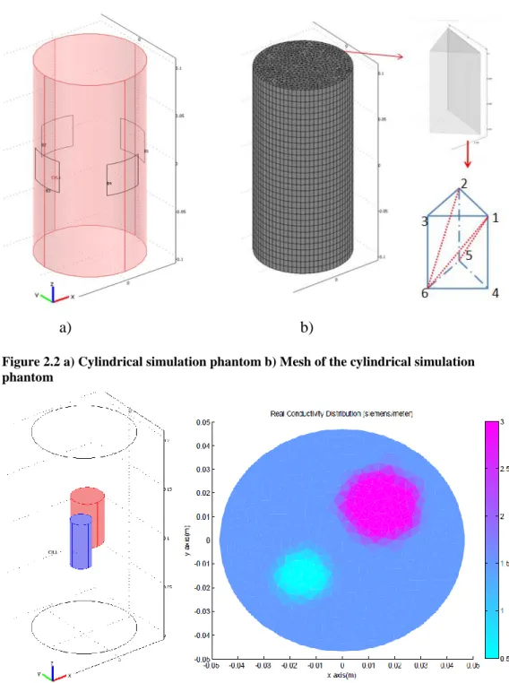
In order to simulate the Conventional and Modified Sensitivity Matrix Methods, a cylindrical phantom given in Figure 2.2-a with diameter 10cm and height 20cm is used. The 3D mesh of the simulation phantom is given in the Figure 2.2-b. This mesh consists of 31 layers and each layer consists of 1126 triangular prisms. Also, in order to solve the forward problem, each triangular prism elements are divided into 3 tetrahedron finite elements as shown in Figure 2.2-b Two objects with 1.5 cm and 3cm diameter and 4.5 cm height are placed inside the phantom to form regions which have different conductivity values. The positions of the objects inside the phantom and the conductivity distribution at

13

the center slice is given in Figure 2.3. Magnetic field is calculated at the center axial slice of this phantom. Since magnetic field is related to magnetic flux density by a magnetic permeability constant, both of these are used in simulations throughout the thesis.

a) b)

Figure 2.2 a) Cylindrical simulation phantom b) Mesh of the cylindrical simulation phantom

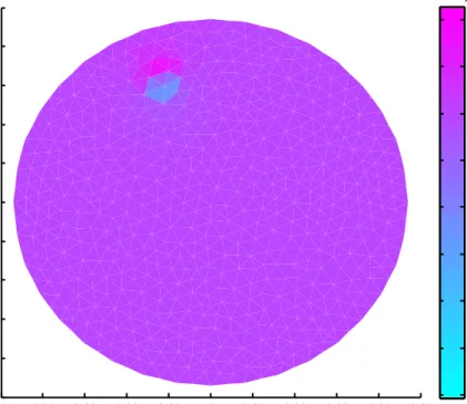
Figure 2.3 a) Position of the objects placed in to the phantom simulation phantom b)The real conductivity distribution at the center slice of the phantom

14

2.3.1 Sensitivity Analysis in z-direction

The sensitivity of the magnetic field to the conductivity of an element can be defined as the change in magnetic field due to the change in conductivity of that element. In Figure 2.4 the sensitivity of the center slice magnetic field to an element which is located in the center slice is given.

-0.05 -0.04 -0.03 -0.02 -0.01 0 0.01 0.02 0.03 0.04 0.05 -0.05 -0.04 -0.03 -0.02 -0.01 0 0.01 0.02 0.03 0.04 0.05 x axis (m)

Change in Hz for a Small Conductivity Change in a Triangular Prism at the Center Slice

y a x is ( m ) -6 -5 -4 -3 -2 -1 0 1 2 x 10-5

Figure 2.4 The sensitivity of the center slice magnetic field to an element which is located in the center slice is given

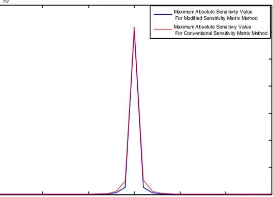
It is desired to investigate how the sensitivity of the center slice magnetic field depends on the conductivity of an element as the distance of the element to the center slice is varied. For this purpose the conductivity of elements on a vertical

line are changed one by one and for each element ΔH is calculated. Then, the z

maximum value of ΔH is calculated. Finally, maximum of z ΔH values are z

plotted for each element with respect to the distance of the elements to the center slice.

15

From the plot in Figure 2.5 it is seen that if the distance of the element to the center slice is zero, the sensitivity of the center slice magnetic field to the change in the conductivity of the element is maximum. Although the sensitivity of the center slice magnetic field to the elements in the ± 2 layer range still remains significant, the sensitivity of the center slice magnetic field to the

elements’ conductivity becomes negligible after 2 layers distance. Therefore,

assumptions for conductivity of the elements which are away from the center slice, do not change calculated magnetic field at the center slice significantly. Our assumption is that conductivity is not changing in the z direction. It is assumed that the triangular prisms which are in the same x, y coordinates have the same conductivity values. With this assumption, three dimensional problem is reduced to two dimensional form which results in reduction in the number of unknown from 34906 to 1126. Here 34906 is the total number of prisms and 1126 is the number of prisms in each layer.

-15 -10 -5 0 5 10 15 0 1 2 3 4 5 6 7x 10 -5

distance of the element to the center slice (slice)

M a x im u m A b s o lu te S e n s it iv it y V a lu e

Maximum Absolute Sensitivity Value For Modified Sensitivity Matrix Method Maximum Absolute Sensitiviy Value For Conventional Sensitivity Matrix Method

Figure 2.5 Distance of the element to the center slice of the phantom (slice) versus the maximum absolute sensitivity value of the center slice magnetic field to the element.

16

2.3.2 Comparison of the Conventional Sensitivity Matrix Method

with the Modified Sensitivity Matrix Method

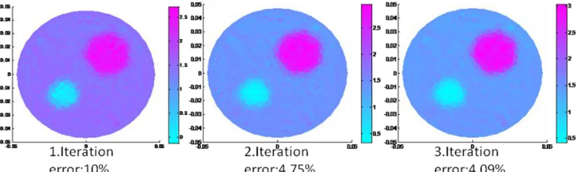
For simulations, the forward 3D problem for the real conductivity distribution is solved to find Hz. And a Gaussian noise is added to the acquired magnetic field to represent noise which might be accumulated due to the MRI system. For the conventional sensitivity matrix method after three iterations conductivity distribution at the center slice of the phantom is found with %4.09 error percentage. Found conductivity distribution after each iteration step are shown in Figure 2.6. These three iterations take 39 minutes.

Figure 2.6 Conductivity distributions acquired using the Conventional Sensitivity Matrix Method for the three iteration

Convergence of the conductivity distribution and magnetic field versus iteration number for the Conventional Sensitivity Matrix Method is given in Figure 2.7.

Figure 2.7 Convergence of the conductivity distribution and magnetic field versus iteration number for the conventional sensitivity matrix method

17

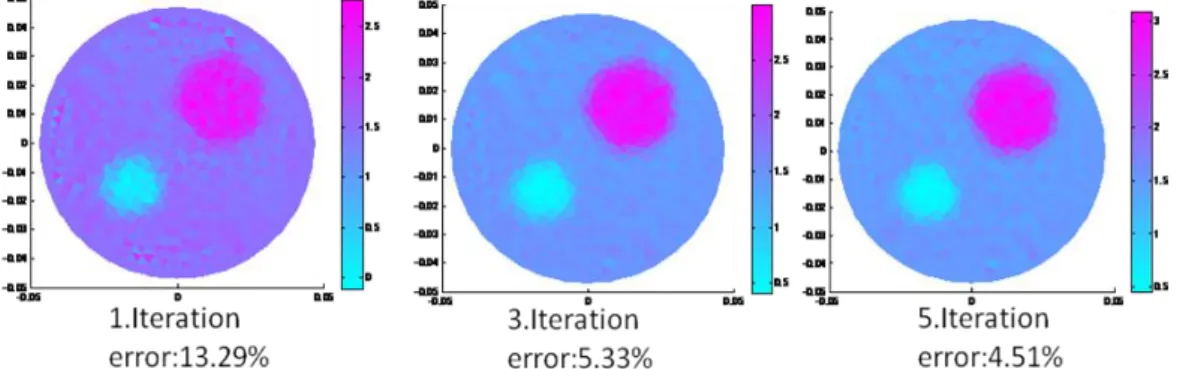
On the other hand, using the Modified Sensitivity Matrix Method it is possible to reconstruct conductivity distribution with the same error percentage (%4.59 ) within 1.3 minutes. Conductivity distribution acquired at the center slice of the phantom for three of the five iteration steps are shown in Figure 2.8.

Figure 2.8 Conductivity distributions acquired using the Modified Sensitivity Matrix Method for the three iterations (1,3 and 5. iterations)

Convergence of the conductivity distribution and magnetic field versus iteration number for the Modified Sensitivity Matrix Method is given in Figure 2.9.

Figure 2.9 Convergence of the conductivity distribution and magnetic field versus iteration number for the modified sensitivity matrix method

In general, the Conventional Sensitivity Matrix Method requires about three iterations to converge a solution. On the other hand, the Modified Sensitivity Matrix Method requires from five to ten iterations to converge the same

18

solution. However, the Modified Sensitivity Matrix Method still necessitates less time than the conventional one. This is because of the fact that each iteration of the Modified Sensitivity Matrix Method takes significantly less time than the conventional one.

19

Chapter 3 : Multichannel Current

Source for MREIT

In MREIT, the use of uniform internal current distribution is important in order to reconstruct less noisy conductivity distributions. However, uniform current distribution cannot be obtained by using a classical single channel current source. Also, using single channel current source results in sudden magnetic flux density changes around the electrodes. Measurements of magnetic flux density have artifacts due to this sudden changes in the magnetic flux density. Also, it is more likely to observe errors in calculation of the magnetic flux density around the regions where the magnetic flux density changes rapidly. Another problem with

using the single channel current source is that calculated ΔB might be more z

sensitive to geometry errors made in the simulation which is used to calculate magnetic flux density for the uniform conductivity distribution. In this thesis, the use of the multichannel current source is proposed in order to reduce the errors in

z

ΔB which are arising from the geometry mismatches, measurement artifacts and

inaccuracies in calculations. The use of the multichannel current source reduces these errors by producing a nearly uniform current distribution even around the electrodes.

3.1 Effects of Errors in Boundary and Electrode Positions to the

Difference Magnetic Field

As mentioned earlier in the algorithms of the Conventional Sensitivity Matrix Method and the Modified Sensitivity Matrix Method, the Sensitivity Matrix

Method requires to subtract calculated magnetic flux density B from the _z

measured one. The success of the sensitivity matrix algorithm depends on the

correctness of the calculation of ΔB . If the initial conductivity assumption is _z

subtracted from the real conductivity distribution, the difference should generate

z

ΔB . However, if the boundary of the simulation object is different than the real

objects' boundary, in ΔB also a difference occurs due to this boundary _z

20

different types of current profiles, and these different current profiles create different magnetic flux density distributions. Therefore, these boundary

mismatches cause ΔB distribution whose values are different than zero. Since _z

z

ΔB is not correct, the calculated conductivity values are also faulty. In order to

minimize these faults, the effects of the certain boundary mismatches are investigated. This work consists of solving the forward problem for several

possible boundary mismatch cases and calculating resulting error on ΔB . For _z

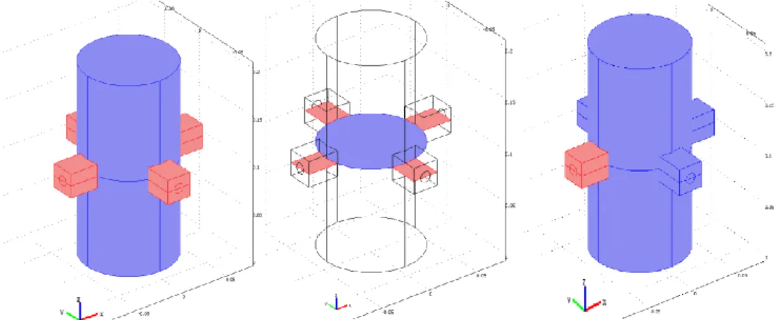
simulations a cylindrical phantom with recessed electrode regions is used. In Figure 3.1-a the simulation phantom is shown with its recessed parts (pink shows recessed electrode regions). Also, the electrodes are shown on the recessed region

with circles. Errors in ΔB are calculated at the circler region of the center slice _z

which is shown at Figure 3.1-b.

a. b. c.

Figure 3.1 a) Simulation phantom with recess electrode parts b) Center slice of the simulation phantom c) Selected recess part of the phantom

In order to calculate boundary mismatch effects on ΔB , z B is calculated at the z

center slice of a phantom with uniform conductivity distribution. This phantom represents the real conductivity distribution and real boundary condition. So, the

calculated B is assigned as the real magnetic flux density at the center slice of _z

this phantom. The maximum absolute value of this B distribution is found as _z

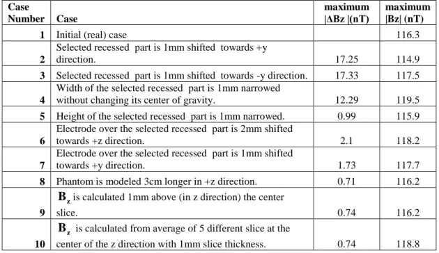
116.3 nT. In order to simulate boundary mismatch cases, for each case the

21

Afterwards, subtracting the new B from the real one and taking its absolute _z

value ΔB is calculated. Maximum values of _z ΔB for each case are shown in _z

Table 3.1. In order to clarify defined cases in Table 3.1, the 1mm shift of selected recessed part towards +y direction is shown in Figure 3.2 (Selected recessed part of the phantom is shown in Figure 3.1-c with pink color.).

Figure 3.2 "1 mm" shift of the selected recess part towards to +y direction

Case Number Case maximum |ΔBz |(nT) maximum |Bz| (nT)

1 Initial (real) case 116.3

2

Selected recessed part is 1mm shifted towards +y

direction. 17.25 114.9

3 Selected recessed part is 1mm shifted towards -y direction. 17.33 117.5 4

Width of the selected recessed part is 1mm narrowed

without changing its center of gravity. 12.29 119.5 5 Height of the selected recessed part is 1mm narrowed. 0.99 115.9 6

Electrode over the selected recessed part is 2mm shifted

towards +z direction. 2.1 118.2

7

Electrode over the selected recessed part is 1mm shifted

towards +y direction. 1.73 117.7 8 Phantom is modeled 3cm longer in +z direction. 0.71 116.2

9

z

B is calculated 1mm above (in z direction) the center

slice. 0.74 116.2

10

z

B is calculated from average of 5 different slice at the

center of the z direction with 1mm slice thickness. 0.74 118.8 Table 3.1 Errors in ΔB_zdue to the wrong definition of the boundary positions

From Table 3.1 it is seen that the errors made at the intersection of the cylindrical part of the phantom with the recess part, create more errors in the

22

calculation of B . According to the results which are shown in Table 3.1 other _z

geometry mismatches do not have significant effects on the error in B . _z

However, the intersections of the recess parts with the cylindrical part represents the electrode positions when there is no recess part for the electrodes. So, if there is no recess part, the errors in the position of the electrodes cause high

z

ΔB errors around the electrode region.

3.2 Known Problems with Single Channel Current Source in

MREIT

As mentioned earlier in order to create magnetic flux density inside the imaging object, it is needed to inject current into the object. However, the current injection profile which uses a single electrode pair to inject current into an object have some problems. First of all, uniform current distribution which is preferable for MREIT applications, cannot be obtained using this current injection profile. Secondly, due to the single electrode pair profile, the boundary

mismatches especially around the electrodes produce high errors in ΔB ,which _z

is important for the algorithms running based on ΔB . Also, the rapid changes _z

in B around the electrode cause high errors in Laplace of the z B . These errors z

affect the algorithms which are using Laplace of the B . Finally, the applied _z

current to the electrodes is not distributed uniformly over the electrode, instead most of the current is injected around the edges of the electrodes.

Some of the MREIT reconstruction algorithms use measured current distribution in order to reconstruct conductivity distribution. For these algorithms the magnitude of the current holds a critical role. Found conductivity values are not reliable in the regions where the magnitude of the current is low. Due to the fact that the current distribution inside the object cannot be controlled with known current injection profiles, it is likely to observe that some regions inside the object have low current density distribution. For these regions calculated conductivity values are not reliable.

23

Injecting current into the object through small flat electrodes is the worst case of using a single electrode pair. In this case, current density is concentrated around the electrodes, which leads to a current density profile which is far away from being uniform. In order to sustain uniform current distribution for the region of interest, it might be useful to use larger electrodes which are large enough to cover the boundary of the region of interest. However, injected current through the surface of the electrodes are not constant over the surface of the electrodes. Most of the current is injected from the edges of the electrodes. So, injected current is still not uniform even near the electrode surface. A uniform current density electrode is proposed by Song at al [7] to ensure uniform current distribution over the surface of the electrode. However, current profile over the surface of electrode is also determined by the conductivity distribution under the electrode. In other words, current distribution over the surface of the electrode can be uniform when the conductivity distribution under the electrode is uniform. As mentioned above, it is preferable to have uniform current distribution around the region of interest which cannot always be sustained by uniform current electrodes. This is because of the fact that current distribution inside the object depends on not only the current distribution over the surface of the electrode but also the geometry of the object, and the conductivity distribution inside the object. So, even with uniform current density electrodes it might not be possible to generate a uniform current distribution inside the object.

Also, some of the MREIT algorithms directly reconstruct conductivity

distribution from z component of the measured magnetic flux density (B ). _z

Among these algorithms some of them require solving the magnetic field intensity for known boundary and an initial conductivity distribution

assumption. The next step in these algorithms, is subtracting the simulated B z

24

current into the object, there might be too much difference in ΔB around the _z

electrodes. Since B magnitude is very high and very variable around the _z

electrodes, these regions are too sensitive to any boundary mismatch.

As mentioned earlier if the current is applied from a classical single electrode pair, current density is concentrated around specific regions, which leads to a rapid change in current density around these regions. This rapid change in

current results in rapid change in B , which causes more errors around the _z

electrodes with respect to the other regions in Laplace of B . _z

3.3 Using Multichannel Current Source in MREIT

In order to solve the problems occurring due to the single electrode pair current injection profile, the use of a multichannel current source is suggested. Using multiple electrode pairs (channel) to inject current into the object, allows to control current distribution inside the object that we want to image. On the other hand, if the current is applied from a single electrode pair, it is not possible to control current distribution inside the object. Some of the MREIT algorithms reconstruct the conductivity values from the current distribution. These algorithms are not reliable for the regions where the current density is low. Therefore, it is crucial to control current distribution inside the object. Also, by using multichannel current injection profile, it is possible to distribute total current among many electrodes. When the current is distributed among many

electrodes, magnitude of B around the electrodes is low. But it is higher when _z

the total current is injected through one electrode pair. Algorithms requiring

subtracting simulated B from the measured _z B , are more sensitive to boundary _z

definition errors for the regions where B magnitude changes rapidly. So, _z

injecting current through multiple electrodes decreases the algorithms' sensitivity to boundary mismatches between the simulation and reality.

25

3.4 Experiment: investigation of the effect of the multi channel

current source on

3.4.1 Acquisition of the z component of the magnetic flux density

(

)

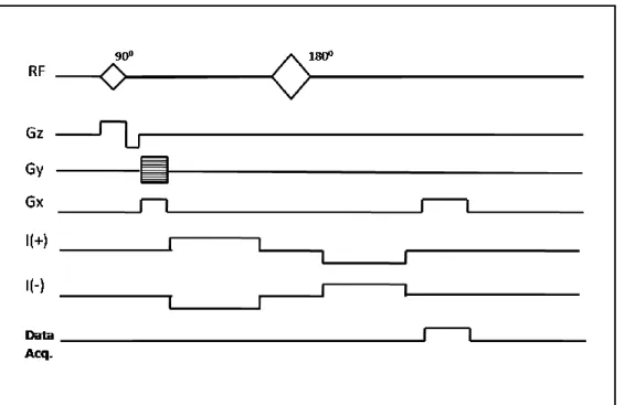
In the experiments, the standard spin-echo pulse sequence (Figure 3.3) is used to

acquire MRI images. In order to acquire a B distribution at a slice which arise _z

from the current injection, two MRI images are acquired at that slice. For these two acquisitions, currents of opposite polarities (I(+), I(-)) are applied for a total

duration of T . In Figure 3.3, spin echo pulse sequence and the current _c

waveforms of I(+) and I(-) for two acquisitions are shown. As a result of these current injections, the acquired images take the form below:

( , ) ( , ) exp( ( , )) exp( ( , ) )_c

M x y m x y j x y jB_z x y T

Here m x y( , ) is the transverse magnetization, ( , )x y is the systematic phase

artifact,  is the gyromagnetic ratio, and B is the magnetic flux density which _z

arises from the current injection. The phases of these two images are given below in radians.

1 ( , )x y  ( , )x y Tc

   Bz

2 ( , )x y  ( , )x y Tc

   Bz

From these two phases B can be calculated as _z B_z( , )x y    ( _{1 2}) / (2T_c).

26

Figure 3.3 Spin echo pulse sequence and current injections for positive and negative directions.

3.4.2 Experimental procedure and results

Figure 3.4 Cubic phantom with multiple electrodes

Two experiments are conducted to show that multichannel current source

27

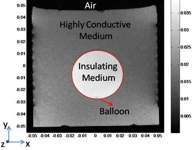
calculation of magnetic flux density for a uniform case and measurement artifacts. In the first case, the current is injected into the object through six electrode pairs while in the second case, the current is injected into the object through thirty electrode pairs. In both of the experiments a cubic phantom

shown in Figure 3.4 filled with 12gr/L agar, 12gr/L NaCl, 1gr/L CuSO4 and

distilled water is used. As an object, a plastic balloon filled with 12gr/L NaCl,

1gr/L CuSO4 and distilled water is used. Since the plastic balloon is not

conductive, the phantom consists of highly conductive and insulating conductivity regions. These regions are shown in Figure 3.5 on the MRI

magnitude image. MRI parameters are chosen as TR: 900 ms, TE: 60 ms, Tc=

42 ms, FOV: 150 mm, Resolution: 256*256, Slice Thickness: 5 mm. In the first experiment 19mA total current is injected through the six electrode pairs shown at the top left of the Figure 3.6. From each electrode pair the same amount of current is injected into the object which is around 3.17mA. At the top right of

the Figure 3.6 the z component of the magnetic flux density (B ) distribution z

acquired from MRI system for six electrode current injection profile is shown.

z

B distribution is calculated for the uniform conductivity distribution and six

electrode current injection profile. This B distribution is shown at the bottom- _z

left of the Figure 3.6. If we subtract B acquired in the experiment, from the z

z

B calculated at the simulation, ΔB is obtained at the bottom left of the Figure _z

3.6. As expected, a B difference can be observed around the object due to its _z

conductivity difference. However, around the electrodes, there are unexpected

z

B differences due to the mismatches of the electrode positions. In the second

experiment, the same amount of the total current (19mA) is injected in to the object from thirty electrode pairs which are shown at the top left of the Figure 3.6. From each electrode pair the same amount of current is injected to the

object which is around 0.63mA per channel. In this case B acquired from MRI, _z

and B calculated from the simulation for a uniform case are shown at the top _z

28

magnetic flux density ΔB calculated in this part of experiment is shown at the _z

bottom left of the Figure 3.7. As expected, there is a difference in ΔB around _z

the object due to the difference of the conductivity of the object. As opposed to

the first part of the experiment, there is no B difference around the electrodes. _z

So we can conclude that the multichannel current source reduces the errors around the electrode region due to the boundary mismatches, calculation inaccuracies and measurement artifacts.

29 -0.06 -0.04 -0.02 0 0.02 0.04 0.06 -0.05 -0.04 -0.03 -0.02 -0.01 0 0.01 0.02 0.03 0.04 0.05 -1.5 -1 -0.5 0 0.5 1 1.5 x 10-7 0 50 100 150 200 250 50 100 150 200 250 -1 -0.8 -0.6 -0.4 -0.2 0 0.2 0.4 0.6 0.8 1 x 10-7 -0.06 -0.04 -0.02 0 0.02 0.04 0.06 -0.05 -0.04 -0.03 -0.02 -0.01 0 0.01 0.02 0.03 0.04 0.05 -1.5 -1 -0.5 0 0.5 1 1.5 x 10-7

Figure 3.6 Electrodes used to inject current into the object and imaging slice (Top Left) The magnetic flux density difference acquired for the six electrode current injection profile. (Bottom Left) The magnetic flux density measured for the six electrode current injection profile (Top Right) The magnetic flux density calculated for the six electrode current injection profile and uniform conductivity distribution (Bottom Right)

30 -0.06 -0.04 -0.02 0 0.02 0.04 0.06 -0.05 -0.04 -0.03 -0.02 -0.01 0 0.01 0.02 0.03 0.04 0.05 -8 -6 -4 -2 0 2 4 6 8 x 10-8 0 50 100 150 200 250 50 100 150 200 250 -1 -0.8 -0.6 -0.4 -0.2 0 0.2 0.4 0.6 0.8 1 x 10-7 -0.06 -0.04 -0.02 0 0.02 0.04 0.06 -0.05 -0.04 -0.03 -0.02 -0.01 0 0.01 0.02 0.03 0.04 0.05 -8 -6 -4 -2 0 2 4 6 8 x 10-8

Figure 3.7 Electrodes used to inject current into the object and imaging slice (Top Left) The magnetic flux density difference acquired for the multiple (30) electrode current injection profile. (Bottom Left) The magnetic flux density measured for the multiple (30) electrode current injection profile (Top Right) The magnetic flux density calculated for the multiple (30) electrode current injection profile and uniform conductivity distribution (Bottom Right)