Deep learning approaches for MRI image classifications

T.C.

ANTALYA BILIM UNIVERSITY

INSTITUTE OF POSTGRADUATE EDUCATION

DISSERTATION MASTER’S PROGRAM OF ELECTRICAL AND

COMPUTER ENGINEERING

DEEP LEARNING APPROACHES FOR MRI IMAGE CLASSIFICATIONS

DISSERTATION

Prepared By

Muhammad ZUBAIR

T.C.

ANTALYA BILIM UNIVERSITY

INSTITUTE OF POSTGRADUATE EDUCATION

DISSERTATION MASTER’S PROGRAM OF ELECTRICAL AND

COMPUTER ENGINEERING

DEEP LEARNING APPROACHES FOR MRI IMAGE CLASSIFICATIONS

DISSERTATION

Prepared By

Muhammad Zubair

181212008

Dissertation Advisor

Asst. Prof. Dr. Shahram Taheri

APPROVAL/NOTIFICATION FORM

ANTALYA BİLİM UNIVERSİTY

INSTITUTE OF POST-GRADUATE EDUCATION

MUHAMMAD ZUBAIR, a M.Sc. student of Antalya Bilim University, Institute of Post Graduate Education, Electrical and Computer Engineering owning student ID 181212008, successfully defended the thesis/dissertation entitled “DEEP LEARNING APPROACHES FOR MRI IMAGE CLASSIFICATIONS”, which he prepared after fulfilling the requirements specified in the associated legislations, before the jury whose signatures are below.

Academic Tittle, Name-Surname, Signature rf. Dr. Name SURNAME

Thesis Advisor : Asst. Prof. Dr. Shahram TAHERI,………..

Jury Member : Asst. Prof. Dr. Taner Danışman,………

Jury Member : Asst. Prof. Dr. Jehad Mahmoud HAMAMREH,……….

Director of the Institute : Prof. Dr. İbrahim Sani MERT………..

Date of Submission: 02/11/2020 Date of Defense: 19/11/2020

ABSTRACT

DEEP LEARNING APPROACHES FOR MRI

IMAGE CLASSIFICATIONS

Although there is no treatment for Alzheimer’s disease (AD), but an accurate early diagnosis is very important for both the patient and public care. Our proposed model consists of two main experiments traditional machine learning and deep learning approaches. These two studies were carried out using the Alzheimer’s disease Neuroimaging Initiative (ADNI) dataset. In our first experiment, we tested different handcrafted feature descriptors to diagnose Alzheimer’s disease. But the most powerful and efficient descriptor is Monogenic Binary Coding (MBC) that gives maximum accuracy of 90.14 percent. In the second experiment, we propose a novel deep convolutional neural network for the diagnosis of Alzheimer’s disease and its stages using magnetic resonance imaging (MRI) scans. In this research, we propose a novel 3-way classifier to discriminate patients having AD, mild cognitive impairment (MCI), and normal control (NC) using a pre-trained CNN architecture Inceptionv3. The proposed method work on proficient technique to use transfer learning to identify the images by fine-tuning a pre-trained CNN architecture, Inceptionv3. The performance of the proposed system is calculated over the ADNI dataset. The proposed model showed novel results by giving the best overall accuracy of 95.71% for multiclass classification problems. Our experimental results show that the performance of the deep learning approaches is comparatively higher than the traditional machine learning.

Index Terms: Convolutional Neural Network, Machine Learning, Deep Learning, Transfer

DEDICATION AND ACKNOWLEDGMENT

I dedicate this thesis to my parents, friends, and teachers who always supported me to this day of my life.

I am very grateful to my advisor Asst. Prof. Dr. Shahram Taheri who guided and encouraged me throughout the thesis, who opened the doors for me in this field of research.

I would also like to thank the jury members Asst. Prof. Dr. Taner Danışman and Asst. Prof. Dr.

CONTENTS

2.1 Traditional Machine Learning Approaches...3

2.2. Deep Learning Approaches...6

3. BACKGROUND MATERIALS...11

3.1 Deep Learning...11

3.2 Neural Network...11

3.3 Convolutional Neural Network (CNN)...12

3.4 Transfer Learning...14 3.5 CNN Architecture...15 3.5.1 Google Net...15 3.5.2 ResNet...17 3.5.3 Inception V3 (and V2)...18 3.5.4 DenseNet...20 3.5.5 MobileNetV2...20

3.6 Hand-Crafted Feature Descriptors...22

3.6.1 Binary Pattern of Phase Congruency (BPPC)...22

3.6.2 Gradient Local Ternary Pattern (GLTP)...22

3.6.3 Gradient Direction Pattern (GDP)...22

3.6.4 Local Arc Pattern (LAP)...23

3.6.5 Local Binary Pattern (LBP)...23

3.6.6 Local Gradient Increasing Pattern (LGIP)...23

3.6.7 Local Gradient Pattern (LGP)...23

3.6.8 Local Monotonic Pattern (LMP)...24

3.6.9 Local Phase Quantization (LPQ)...24

3.6.10 Monogenic Binary Coding (MBC)...24

3.6.11 Median Binary Pattern (MBP)...24

3.6.13 Weber Local Descriptor (WLD)...25 3.7 Information Fusion...25 3.7.1 Feature-level Fusion...26 3.7.2 Decision-level Fusion...27 4. PROPOSED METHOD...28 4.1 Dataset...28

4.2 Proposed Monogenic Binary Coding (MBC)...30

4.3 Proposed CNN Architecture: Inceptionv3...31

4.3.1 Parameters of Transfer Learning...31

4.3.2 Modified Network Architecture...32

4.3.3 Network Training and Fine Tuning...34

4.3.4 Network Performance and Complexity...34

5. EXPERIMENTAL RESULTS...36

5.1 Results of Hand-Crafted descriptors...36

5.2 CNN Architecture Results...40

6. DISCUSSION...52

Future Work...53

Conclusions...53

INSTITUTE OF POSTGRADUATE EDUCATION

ELECTRICAL AND COMPUTER ENGINEERING

MASTER PROGRAM WITH THESIS

ACADEMIC DECLARATION

I hereby declare that this master’s thesis titled “Deep Learning Approaches for MRI Image Classifications” has been written by myself under the academic rules and ethical conduct of the Antalya Bilim University.

I also declare that the work attached to this declaration complies with the university requirements and is my work.

I also declare that all materials used in this thesis consist of the mentioned resources in the reference list. I verify all these with my honor.

02/11/ 2020 Muhammad ZUBAIR

LIST OF FIGURES

Figure 1: Learning curve with MRI biomarker as features [6]...3

Figure 2: Binary and multi-class classification tasks [7]...4

Figure 3: Performance Analysis between Coronal, Sagittal and Axial planes [8]...5

Figure 4: Results comparisons of different techniques [13]...8

Figure 5: Performance Analysis in terms of accuracy, sensitivity and specificity [14]...9

Figure 6: Neural Network...12

Figure 7: An Architecture of Convolutional Neural Network (CNN)...13

Figure 8: GoogleNet Inception Module [20]...16

Figure 9: Two successive 3×3 convolutions and 5×5 convolution [20]...16

Figure 10: Residual learning block [21]...17

Figure 11: Decomposition of 5×5 filters into multiples 3×3 filters [20]...18

Figure 12: New Inception Module...19

Figure 13: Final Pooling layer...19

Figure 14: Different layers of DenseNet to learn features [22]...20

Figure 15: Feature-level image fusion...26

Figure 16: Decision-level Image fusion...27

Figure 17: MRI data into three different 2D planes (a) Axial, (b) Coronal, and (c) Sagittal...29

Figure 18: Classification of MRI images in 3-way classifier AD, NC, and MCI...30

Figure 19: Proposed Methodology...32

Figure 20: Transferring CNN Layers...33

Figure 21: Result of GoogleNet using an axial plane...40

Figure 22: Result of Resnet18 using an axial plane...41

Figure 23: Result of Resnet101 using an axial plane...41

Figure 24: Result of Densenet201 using an axial plane...42

Figure 25: Result of Mobilenetv2 using an axial plane...42

Figure 26: Result of Inceptionv3 using an axial plane...43

Figure 27: Result of GoogleNet using the coronal plane...44

Figure 28: Result of Resnet18 using the coronal plane...45

Figure 29: Result of Resnet101 using the coronal plane...45

Figure 30: Result of Densenet201 using the coronal plane...46

Figure 31: Result of Mobilenetv2 using the coronal plane...46

Figure 32: Result of Inceptionv3 using the coronal plane...47

Figure 33: Result of GoogleNet using the sagittal plane...48

Figure 34: Result of Resnet18 using the sagittal plane...49

Figure 35: Result of Resnet101 using the sagittal plane...49

Figure 36: Result of DenseNet201 using the sagittal plane...50

Figure 37: Result of Mobilenetv2 using the sagittal plane...50

LIST OF TABLES

Table 1: Comparison of Proposed Method results with the region and voxel-based method...6

Table 2: Performance evaluation of different modalities of AD with MR and PET...7

Table 3: Neural Network Confusion Matrix...8

Table 4: Performance Analysis between traditional and deep learning techniques...10

Table 5: Architecture of MobileNetV2 [23]...21

Table 6: Information of dataset...29

Table 7: Results of Axial, Coronal and Sagittal planes using cell size 2...36

Table 8: Results of Axial, Coronal and Sagittal planes using cell size 3...37

Table 9: Results of Axial, Coronal and Sagittal planes using cell size 5...38

Table 10: Results of Axial, Coronal and Sagittal planes using cell size 10...39

Table 11: Results of pre-trained CNN Architecture using an axial plane...43

Table 12: Results of pre-trained CNN Architecture using a coronal plane...47

Table 13: Results comparison between axial, coronal and sagittal planes...51

ABBREVIATIONS

CNN Convolutional Neural Networks

ADNI Alzheimer’s disease Neuroimaging Initiative

MCI Mild Cognitive Impairment

NC Normal Control

MBC Monogenic Binary Coding

MBP Median Binary Pattern

LAP Local Arc Pattern

MLP Multilayer Perceptron

BPPC Binary Pattern of Phase Congruency

GLTP Gradient Local Ternary Pattern

GDP Gradient Direction Pattern

LBP Local Binary Pattern

LGP LMP LPQ MTP WLD LGIP

Local Gradient Pattern Local Monotonic Pattern Local Phase Quantization Median Ternary Pattern Weber Local Descriptor

1.

INTRODUCTION

Alzheimer's disease (AD) is a very severe form of dementia, it is a very complicated disease that gradually damages brain cells and affecting memory and thinking skills to destroy, and in the end the ability to do basic tasks [1]. Dementia varies in intensity from the initial level, in which the hippocampus is one of the most important regions of the brain to be damaged by short-term memory loss and other mental deterioration and by nerve cell damage to the brain [1]. It affects the most extreme level when there is significant hippocampus shrinkage, because in which the person relies on others to complete the routine works. AD causes significant challenges with human thinking, learning, and daily works. Because of the relentless annihilation of nerve cells over time, basic human mental capabilities are brutally decreased for the rest of their life. AD is expected to affect 1 out of 85 people worldwide by 2050, with an estimated rise of more than 100 million by 2050 [2]. It is expected that 5.3 million people in 2014 of all ages who have AD. Alzheimer's disease is the sixth largest cause of death in the US. Alzheimer’s disease prevalence varies among several different aspects, including age, co-morbidity, society, and level of education.

There is no treatment for AD, but encouraging early diagnosis research and development are underway. Advanced neuroimaging techniques have been developed for detecting structural and molecular AD-related bio-marks, including magnetic resonance imaging (MRI) and positron emission tomography (PET). We can discover the disease early by MRI, it's a technique that uses a magnetic field and radio waves to build a detailed 3D image of the brain. MRI is a non-intrusive way of seeing changes in the brain atrophy, which was commonly used in AD research due to its strong spatial resolution, improved usability, high contrast, and no radiation during the scanning process. Despite much research, there is no definitive diagnosis in current clinical practice because of similar and inconsistent symptoms. The presence of AD can only be verified by post-mortem analysis of the brain tissue after the patient's death. Thus, an accurate early diagnosis of AD is very important for patient and social care and becomes even more common once the treatments are available to reverse progression of the disease.

1.1 Motivation

The early diagnosis of AD depends on the model's results. CNN and deep learning motivate the latest researchers in computer vision and machine learning. As we discussed before, there is no treatment for AD and there is no proper diagnosis in current clinical practice. AD can only detect after the death of the patient through a post-mortem analysis. To overcome such problems, a computer diagnosis algorithm is being proposed using CNN (convolutional neural network) a machine learning technique. It is a technique of learning that helps a computer to learn typical representation from raw data. The hierarchical layered structure of the network is the reason behind the popularity. Inspired by the visual structure of humans, the Convolutional Neural Network (CNN) learns the features from the compositional hierarchy, from the simple edges and evolving into a more complicated form. A stack of convolutional and pooling layers is provided. Each convolutional layer identifies local conjunctions of features from the previous layers and pooling merge the identical feature into one by diminishing the feature map.

1.2 Contributions

There are three main contributions to this work. We first convert 3D NIFTI format MRI data into 2D JPEG images in three different planes axial, coronal, and sagittal. In this study, we performed experiments on all these three planes to get optimal results and this is a novel approach. Secondly, we reviewed different handcrafted feature descriptor techniques to extract the features on different cell sizes to get the maximum results. Lastly, we experiment with different pre-trained CNN architecture and we achieved maximum accuracy of 95.71% from the pre-trained Inceptionv3 model that is superior to the other similar approaches in the literature.

1.3 Thesis Organization

The paper is organized as follows: The literature review is discussed in Chapter 2, while Chapter 3 describes the different background methods (Neural Networks, CNN and its architecture, Hand-crafted Feature Descriptors, Transfer Learning, Information Fusion, etc.) that we apply on the proposed system. The information about the dataset and proposed approaches such as Hand-crafted Feature Descriptors and Convolutional Neural Network is discussed in section 4. Moreover, the results of the proposed approaches are described in section 5 and discussion about the results of the proposed methods and previously applied methods along with the future work are described in Chapter 6.

2.

LITERATURE REVIEW

In the clinical imaging domain and the diagnosis of Alzheimer’s disease is crucial, not convenient for ensuring individual mental ability, but also for public health. Recently, various techniques have been presented for the analysis of AD such as traditional machine learning and deep learning approaches. Deep learning performs more successfully as compared with traditional learning.

2.1 Traditional Machine Learning Approaches

Sorenson et al. [3] present a 3-way MRI combined biomarker that incorporating multiple different MRI biomarkers (cortical thickness estimations, volumetric estimations, hippocampal structure, and hippocampal surface). The model was created, prepared, and approved utilizing two open-ended reference datasets: the ADNI dataset and the Australian Imaging Biomarkers. In addition, the method was calculated for the diagnosis of computer-aided dementia (CADDementia). ADNI and AIBL data gave the results in a 62.7% accuracy for the healthy normal control (NC) using cross-validation subjects MCI and Alzheimer's disease (AD) patients. Fig. 1 shows the average classification accuracy of the ADNI and AIBL dataset with learning curve using MRI data.

Suk et al. [4] proposed a new, deep architecture to remove uninformative features by hierarchically executing sparse multitasking learning. They hypothesize further that the ideal coefficients of regression replicate the comparative significance of features in showing the variables of the objective reaction. In such a manner, in the accompanying hierarchy, they use the ideal regression coefficient learned as attribute weighting factors in one progression and describe a weighted, sparse, multi-task learning system. Finally, they consider the distributional property of samples per class in the sparse regression model and use the vectors for prompt subclass markings as target values. Fig. 2 illustrates the AD, NC and MCI experiments on the ADNI dataset, binary and multi-class classification tasks were performed. The proposed model yields the highest accuracy of 62.93% indicating that AD and NC and MCI can be satisfactorily differentiated by the proposed method.

Figure 2: Binary and multi-class classification tasks [4].

Varma et al. [5] Proposed a classification framework for the selection of features extraction using the Gray-Level Co-occurrence Matrix (GLCM) process for distinguishing between AD and the normal control of NC. They have conducted evaluations on the MRI acquired from the OASIS database to estimate the proposed method. The performance comparison of axial, coronal and sagittal planes is shown in Fig 3. The suggested method yields an average accuracy of 75.71% indicating that AD and NC can be satisfactorily differentiated by the proposed method.

Figure 3: Performance Analysis between Coronal, Sagittal and Axial planes [5].

Dong et al. [6] proposed a new classification system to differentiate between older subjects of Alzheimer's disease, MCI, and NC. The system used 178 MRI subjects, including 97 NC, 57 MCI and 24 AD. Next, all those 3D MRI images were pre-processed with a standardization atlas registered. So gray matter images were taken and 3D images checked. After that, they implemented PCA for feature extraction. By using the Singular Value Decomposition (SVD) algorithm, they extracted 20 principal components from 3D MRI data and extracted 2 PCs from the additional information via Alternating Least Squares (ALS).

They developed a kernel support vector machine decision tree (kSVM-DT) based on 22 features. Particle Swarm Optimization (PSO) had calculated the cost of the error parameter and the kernel parameter σ. The quadratic programming approach also obtained the weights w and biases b. The consequences of the proposed method show that the kSVM-DT achieved 80% classification precision, which is more than 74% without the kernel method. By comparison, the PSO meets the arbitrary sampling process when selecting parameters for the classifier. The period to measure a new patient is just 0.022s.

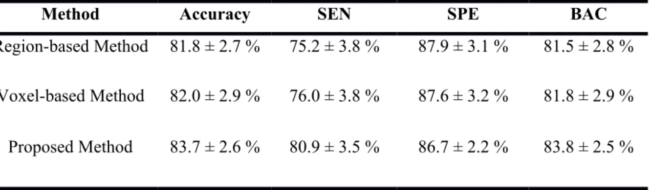
Zhang et al. [7] are used as structural Magnetic Resonance Imaging (sMRI) to diagnose AD by using very impressive and prominent techniques. The success of computer-aided diagnostic approaches utilizing sMRI data largely relies on two time-taking steps: (1) non-linear individualization and (2) segmentation of brain tissue. To reduce this constraint, it proposes a method of removing landmark-based features without involving nonlinear identification and brain tissue segmentation during the training period, group comparisons are carried out first to differentiate between Alzheimer’s subjects and healthy controls (HCs) dependent on the local morphological features to identify areas of the brain with important set of changes. The centers of the classified regions are usually the landmark that effectively separates AD subjects from HCs. By using the analyzed AD objects, the corresponding landmarks can be identified in a test image using an appropriate regression forest algorithm. Morphological features are extracted with the specified AD landmarks to train a support vector machine (SVM), which is capable of predicting the AD state. The method is tested sequentially in studies on landmark identification and classification of ADs. The proposed method detector error is 2.41 mm and the accuracy of the classification is 83.7%. In Table 1, the proposed method results are compared with the region-based and voxel-based method. Finally, the efficiency of the proposed AD classification is equal or even greater than that of the current regional and voxel-based approaches, although the proposed system is 50 times faster.

Table 1: Comparison of Proposed Method results with the region and voxel-based method.

Method Accuracy SEN SPE BAC

Region-based Method 81.8 ± 2.7 % 75.2 ± 3.8 % 87.9 ± 3.1 % 81.5 ± 2.8 % Voxel-based Method 82.0 ± 2.9 % 76.0 ± 3.8 % 87.6 ± 3.2 % 81.8 ± 2.9 % Proposed Method 83.7 ± 2.6 % 80.9 ± 3.5 % 86.7 ± 2.2 % 83.8 ± 2.5 %

2.2. Deep Learning Approaches

The deep learning approaches is a promising way of research because it can automatically classify the complex data at a high level of abstraction. Lui et al. [8] has developed a new computing framework with a deep learning architecture to better diagnose AD. This approach

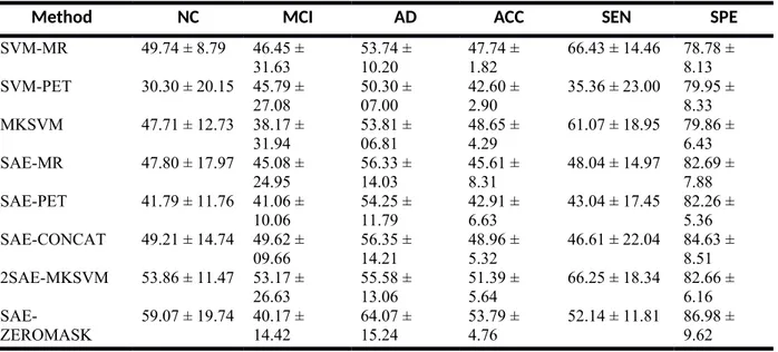
utilizes a zero-masking data fusion strategy to gain additional information from various data modalities. The system can fuse multimodal neuroimaging in one environment and enable fewer labeled data. Performance improvement has been reported in both binary and AD's multiclass classification was observed. Table 2 illustrates the multiclass classification results. The proposed method achieved an overall accuracy of 53.79% and 86.98% specificity.

Table 2: Performance evaluation of different modalities of AD with MR and PET.

Method NC MCI AD ACC SEN SPE

SVM-MR 49.74 ± 8.79 46.45 ± 31.63 53.74 ± 10.20 47.74 ± 1.82 66.43 ± 14.46 78.78 ± 8.13 SVM-PET 30.30 ± 20.15 45.79 ± 27.08 50.30 ± 07.00 42.60 ± 2.90 35.36 ± 23.00 79.95 ± 8.33 MKSVM 47.71 ± 12.73 38.17 ± 31.94 53.81 ± 06.81 48.65 ± 4.29 61.07 ± 18.95 79.86 ± 6.43 SAE-MR 47.80 ± 17.97 45.08 ± 24.95 56.33 ± 14.03 45.61 ± 8.31 48.04 ± 14.97 82.69 ± 7.88 SAE-PET 41.79 ± 11.76 41.06 ± 10.06 54.25 ± 11.79 42.91 ± 6.63 43.04 ± 17.45 82.26 ± 5.36 SAE-CONCAT 49.21 ± 14.74 49.62 ± 09.66 56.35 ± 14.21 48.96 ± 5.32 46.61 ± 22.04 84.63 ± 8.51 2SAE-MKSVM 53.86 ± 11.47 53.17 ± 26.63 55.58 ± 13.06 51.39 ± 5.64 66.25 ± 18.34 82.66 ± 6.16 SAE-ZEROMASK 59.07 ± 19.74 40.17 ± 14.42 64.07 ± 15.24 53.79 ± 4.76 52.14 ± 11.81 86.98 ± 9.62

Deep learning methods (SAECONCAT and SAE-ZEROMASK) supported the precision of NC, MCI and AD. The MCI precision was reduced by 67 out of 331 MCIs, and 102 instances were calculated by their sibling class MCI. SAE-ZEROMASK and MKSVM were very similar in accuracy to MCI. SAE-ZEROMASK improved the overall accuracy by approximately 5 percent compared to the simple concatenation feature (SAECONCAT). The other alternative 2SAE-MKSVM Data Fusion was also carried out in general explicitly.

Manzak et al. [9] wanted to build an automated classification system to test AD using minimal patient data. MRI is widely used for AD diagnosis. MRI is used extensively for diagnosing AD. Different methods are required when considering the cost of the technique and the operational complications. Using Deep Neural Network (DNN), he suggests a fast and effective method to diagnose AD. Reducing algorithm complexity, some of the features were omitted using the Random Forest process. Random Forest's progress is intended to delete DNN features and performance to classify AD. Model for extracting the most significant feature from ADNI data

using standard estimation as training and 24-month testing estimation and afterward applying deep neural networks to the selected features. It reached 67% accuracy by using just 8 of the most important features. Table 3 displays the confusion matrix of the neural network in which 11 patients have AD and 185 patients with NC diagnose correctly.

Table 3: Neural Network Confusion Matrix.

AD NC

AD 11 86

NC 9 185

Young et al. [10] suggested a system for the development of end-to-end learning of the four-differential recognition functions MRI based volumetric convolutional neural network (CNN), PMCI vs. NC, sMCI vs. NC, pMCI vs. SMCI, and AD vs NC. Fig. 4 illustrates the performance of these four differential recognition techniques. The proposed approach was used to solve the classification task pMCI vs. sMCI with convolutional auto-encoder (CAE)-based unsupervised learning for classification process AD vs. NC and supervised transfer learning.

A gradient simulation technique has been used to identify the significance of biomarkers in AD and pMCI, approximating the spatial impact of the CNN model decision. They performed tests on the ADNI database to verify the findings of this report and the results achieved by the proposed approach accuracies of 86.60% and 73.95% respectively for AD and pMCI classification tasks. The progressive parts of the visualization results were recognized in the main regions for classification.

Figure 4: Results comparisons of different techniques [10].

In this model, they primarily use Convolutional Neural Network to identify fMRI clinical evidence on stages of AD and EMCI to those with stable brains that are normal. The usage of MRI data for binary classification has already been completed. The images are divided into three different classes to generalize the classifier. The preprocessing processes proved to be crucial in providing different slicing of 2D images with Normal, EMCI, and AD for greater accuracy in recognizing the most discriminative feature of fMRI brain scans.

Payan et al. [11] developed an algorithm that can diagnose AD brains and healthy brains with input MRI images. It considers deep artificial neural networks class and, more precisely, a group of CNN with sparse autoencoders. The innovative novelty of the proposed method is the use of 3D convolutions on the whole model that gives better results than 2D convolutions. The classification results were obtained through a 3-way classification (AD vs. MCI vs NC) and three differential classifications (AD vs. HC, AD vs. MCI and MCI vs. HC). The average performance of the 3-way classifier is 89.47 percent.

Zhang et al. [12] developed a machine-learning method that allows automatic brain MRI detection. First of all, brain scans including skull removal and spatial normalization were examined. Second, for the volumetric image of one axial slice was selected and then stationary entropy of the wavelet (SWE) was carried out to achieve the properties of the image. Thirdly, a neural network was used as a single hidden layer classifier. Fig. 5 shows the average accuracy of

the AD classification. The proposed method achieved average accuracy of 92.73±1.03 percent, the sensitivity of 92.69±1.29 percent, and specificity of 92.78±1.51 percent.

Figure 5: Performance Analysis in terms of accuracy, sensitivity and specificity [12]. Table 4: Performance Analysis between traditional and deep learning techniques.

Approach Publications Modalities Technique Classification Accuracy

Traditional Machine Learning Approaches

Sorensen et al [3] MRI Combined Biomarkers

3 way (AD/MCI/NC) 62.7% Suk et al [4] MRI+PET+CSF _{DW −S}2

MTL 3 way (AD/MCI/NC) 62.93%

Verma et al [5] MRI GLCM 2 way (AD/NC) 75.75%

Dong et al [6] MRI PCA 3 way (AD/MCI/NC) 80%

Zhang et al [7] MRI Local Morphological features 2 way (AD/HC) 83.07% Deep Learning Approaches

Lui et al [8] MRI SAE-Zeromask 4 way

(AD/cMCI/ncMCI/NC) 53.8%

Manzak et al [9] MRI DNN 2 way (AD/NC) 67%

Young et al [10] MRI CNN 4 way

(AD/pMCI/sMCI/NC)

86.60%

Payan et al. [11] MRI CNN 3 way (AD/MCI/NC) 89.47% Zhang et al [12] MRI CNN 3 way (AD/MCI/NC) 92.73%

Table 4 presents the comparison of the results between traditional machine learning approaches and deep learning approaches. The maximum results achieved from the traditional machine learning is 83.07% whereas the results achieved from deep learning is 92.73%. These experimental results show that the performance of deep learning approaches is better than traditional machine learning. The highest accuracy achieved by Zhang et al [12] using deep learning approach (CNN). The 3-way classification task was performed on ADNI dataset using the MRI images.

3.

BACKGROUND MATERIALS

In this chapter, we will introduce the background of different methods which we will use in multiple studies using techniques such as neural network, convolutional neural network, CNN architecture, transfer learning, and Hand-crafted Feature Descriptors.

3.1 Deep Learning

Machine Learning gives a huge assortment of algorithms from special algorithms along with mathematical approaches such as Bayesian networks, quantitative analyzes such as linear and logistic regression and decision trees. These algorithms are still efficient, but these algorithms have little limitations when learning for very complicated data images. It derives from cognitive theory and information theory and the learning mechanism of human neurons together with strong neuronal interconnection attempts to replicate them. Some of the key benefits of processing neurons and the neural network model are that it can add generalized neurons to any type of data and learn in-depth [13]. It is viewed as a promising way of research because it can classify the complex features at a very abstract point. It involves learning the representation and abstraction of multi-level, useful for data like image, text and sound. One of the extraordinary features in the training process is the opportunity to use unlabeled data [14].

Deep learning is classified as a multi-layer neural network with several neurons on each layer that completes the tasks you want, such as classification, regression, clustering and so on. Each neuron with an activation function is expected to be the logistic node connected to the entry on

the next layer and the loss function is determined to adjust the weights of every neuron in order to make it suitable for data entry. Each layer of multiple neurons in the layer of the neural network started with different weights and simultaneously attempting to learn on input data. Therefore, each node grasps the information from the output of previous layers in multiple layers with separate nodes and slowly losses the estimation of the actual input data to provide a specific outcome [15]. This leads to a great deal of complexity between linked neurons.

3.2 Neural Network

Neural networks are based on neurons that require a weighted sum of the input values. Such weighted sums refer to the scale of significance that performs synapses and merging the specific values in the neuron. However, the neuron only generates the weighted sum. Then there is a real procedure done within the neuron on the combined inputs. This method appears to be a nonlinear function, which generates a neuron output only when the input crosses some thresh-hold. Thus, neural networks apply a nonlinear function by analogy to the weighted sum of the input values. Fig. 6 shows a diagrammatic image of a computational neural network. These values are obtained by the neurons in the input layer and passed to the neurons in the middle layer of the network, which is also called a hidden layer. Finally, the quantities of weight from one or more hidden layers are spread to the output layer which provides users with the final outputs of the network. The outputs of the neurons are often referred to as activations to fit brain-inspired terms for neural networks and the synapses are often called weights.

3.3 Convolutional Neural Network (CNN)

CNN is created by ordinary neural networks. These are composed of neurons with weights that can be trained and biases that can be modified. The growing neuron has certain input features that conduct the dot product and relay features via a non-linearity activation function. There is just a small collection of other neurons in every cell. Such neurons form an image recognition pathway.

It can be compared to viewing a certain part of an image through a telescope. When we see the particular part again, this 'telescope' gets activate and the node weights are changed. The loss function defines the variation in the real measurement. It is obvious from CNN that the inputs are images. This helps one to identify certain elements in the core architecture. It also helps the feed-forward mechanism to be applied more efficiently to decreases the number of network parameters.

Equation (1) represents the error calculation method in the backpropagation step where E denoted error function, x denoted the input, y is ith, jth neuron, Equation l represents layer numbers w is filter weight with c and d indices, N is the number of neurons in a given layer and m is the filter size.

∂ E ∂W_cd=

∑

∑

∑

∑

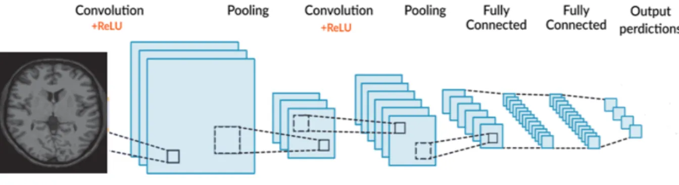
In comparison to a simple neural network, the layers of CNN are organized in distance, height and depth of three-dimensional neurons. The depth is the third volume activation dimension. All scores converge to the class vector by the end of CNN and provide results based on the final class scores. Fig. 7 presents the CNN architecture that includes convolutional layers, pooling layers, and fully connected layers [16].

Figure 7: An Architecture of Convolutional Neural Network (CNN).

Convolution Layer: The convolutional layer's main function is to identify local relations with previous layer features and to map their presence to a feature map. Stride determines how the filter converges with the input volume. The sum of the filter moves by is the phase. Stride is usually set to an integer, not a fraction, in the output number.

When the filter transforms over data height and width, a two-dimensional activation map of the filter is generated. As any filter is transformed, the basic features are known and the weights of each neuron are allocated for the next layers. The neuron also shares parameters with other neurons in the same spatial activation region.

ReLU and pooling layer: ReLU is used on a convolutional layer. The functionality is to translate all negative values to 0. This increases computation efficiency as it improves the problem of gradient descent, where the lower layers work very slowly.

Pooling layer: It extracts important information from large images and shrink images into small size after obtaining important information. A pooling layer is simply a pooling of an image or a series of images. The output has equal numbers of images, but each pixel is smaller. Max-pooling is typically used where the limit of the chosen 2×2 partition matrix is chosen and merged. This layer tackles the problem of overfitting.

Fully-connected Layer: It has all the neuron connections from the previous layers. The activation converges to the individual groups for the preparation of the neural network. The class scores are thus provided and the trained input is expected [17].

3.4 Transfer Learning

Transfer learning is a machine learning methodology in which a model designed for one task is transferred to another task. The idea of transfer learning is to store a different group of trained features on individual data and attempt to utilize the same trained sections of our proposed method. The current standard is the use of pre-trained learning models, as the acquired knowledge significantly reduces training time. Pre-trained CNN on ImageNet Dataset is primarily used for computer vision tasks as computer scientists also make their weights available for the public.

The use of these pre-trained models as extractor features is very common, and the extracted information is then fine-tuned to the respective task. It is divided into three categories [18] [19]:

 CNN Feature Extractor: Here, a pre-trained CNN is taken into our dataset and the last 1000 fully connected layer classification have been removed. This layer is replaced by our special FC layer. The rest of the network is performed as the fixed feature extractor except for the last layer. Then it is transmitted to our locally trained linear SoftMax classifier.

 CNN fine-tuning: It varies significantly different from the above method. In this stage, we remove the last layer and train the last layer but also increase the weight of the pre-trained model. This is an outstanding addition to the model as the weights already tested are fine-tuned to the corresponding input.

 Pre-trained Models: People use regulated weights on their data that are learned in other datasets. Although that is easier and faster in the development process, because the model is not adjusted to the particular situation, the classification accuracy could suffer.

3.5 CNN Architecture

In this section, we will introduce different pre-trained CNN architecture. There are many well-known CNN architectures, most of them earned recognition by achieving good results at the ILSVRCsuch as GoogleNet, Resnet, Inception v3 and v2, DenseNet and mobilenetv2.

3.5.1 Google Net

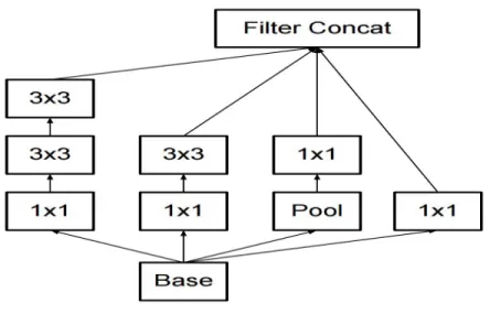
GoogleNet (or the Inception Network) is a 22 layers model designed by Google researchers. GoogleNet was the winner of ILSVRC-2014 ImageNet, where it has proved to be a successful model. The researchers have found a novel approach called the Inception module [20]. The model consists of a simple unit called an "Inception Cell" in which we conduct a sequence of convolutions on various sizes and then add up the results. To save computation, 1x1 convolutions are used to minimize the depth of the input channel. For each cell, we study a range of 1×1, 3×3, and 5×5 filters, and study how to derive features at different scales from the data. Max pooling is often used to maintain the length, but with "same" padding, so that the output can be correctly concatenated. Fig. 8 shows a diagrammatic image of GoogleNet inception module.

Figure 8: GoogleNet Inception Module [20].

Fig. 9 demonstrates the convolutions with wide space filters (for example 5×5 or 7×7) can be useful for the ability to remove features on a larger scale, but it is very costly for calculation. The researchers found that two stacked 3×3 filters will more efficiently reflect a 5×5 convolution.

Figure 9: Two successive 3×3 convolutions and 5×5 convolution [20].

Whereas a 5×5×c filter needs 25c parameters, there are only 18c parameters required for two 3×3×c filters we cannot use nonlinear activation within the two layers of 3×3 to more effectively represent a 5×5 filter. But, it was discovered that linear activation in any respect stages of the factorization was always inferior to using corrected linear units.

3.5.2 ResNet

Kaiming created the Residual Network (ResNet) and was the winner of LSVRC-2015. This came in at the launch of Inception v3 in December LSVRC-2015. The basic concept for ResNet is to feed the output of two consecutive convolution layers AND also bypass feedback into the next layers. Residual blocks that include the residual feature of the intermediate layers of a block affecting the block input. We can find the residual function as a phased improvement, through which we learn how to change the input feature map to better quality applications [21]. Compared to a "simple" network in which new and distinct feature maps for each layer need to be learned if there is no clearing, the intermediate layers should then gradually change their weights to zero such that the residual block becomes an identity function as shown in Fig 10.

Figure 10: Residual learning block [21].

ResNet's main advantage is that hundreds, even thousands of these residual layers can be used to create a network, and trained afterward. That is a little different from ordinary sequential networks, where you find the output enhancements are decreased as you increase the number of layers. For normal feedforward networks, the prediction accuracy decreases as the depth of the network increases [21]. Many variables are responsible for each result, including vanishing of gradient problem, saturation, training data size, and over-fitting. Residual learning allows more than a thousand layers of network depth to become as deep as that. Skip connections make gradient flow easy during the backward pass, and solve the vanishing gradient problem.

3.5.3 Inception V3 (and V2)

Christian and his fellows are extremely professional scholars. Batch-normalized Inception was introduced in February 2015 as Inception V2. Batch-normalization measures the mean and standard deviation at the output of a layer of all feature maps. It involves "blanketing" the test, such that all neural maps have reactions in the same range and a mean of zero. It helps us to learn as the next layer no need to identify offsets in the data and can focus on integrate the best features should be integrated [20].

They announced a new version of the Inception modules in December 2015 and this article provides more information on the implementation choices and illustrates the original GoogLeNet architecture further for the respective architecture. The original concepts are categorized into:

 Maximize network information flow through the careful creation of networks that balance depth and width. Increase maps before any pooling.

 The layer width or the number of features is also increased by increasing the depth.

 To increase the feature combination to the next layer, using the difference in width on each layer.

 Use only 3×3 convolution whereas 5×5 and 7×7 filters can be decomposed with multiples 3×3 filters as shown in Fig. 11.

Figure 11: Decomposition of 5×5 filters into multiples 3×3 filters [20].

Fig. 12 displays the new inception module after the decomposed of 5×5 filter into 3×3 filters.

Figure 12: New Inception Module

Fig. 13 shows that the inception modules decrease the size of data by pooling during the evaluation of inception. This is like performing a parallel convolution with a basic layer of pooling. Inception also uses a final classifier a pooling layer and softmax.

Figure 13: Final Pooling layer

3.5.4 DenseNet

The concept behind the dense convolutional networks is simple: reference maps from earlier times can be useful in the network. Therefore, the feature map of each layer is connected to the input of each successive layer inside a dense block as shown in Fig 14. It enables layers in the network to explicitly use features from previous layers and thereby enables the reuse of features throughout the network [22].

Figure 14: Different layers of DenseNet to learn features [22].

When we first came across this model, we figured that supporting the dense connections between layers would have an absurd number of parameters for supporting. However, because the network can directly use all previous feature maps, the authors found that they could operate with very little depths of the output channel (i.e. 12 filters per layer). The authors refer to the number of filters used in each convolutional layer as a "growing rate," k since each layer would have k channels more than the last (as a consequence of multiplying and concatenating to the input all previous layers). DenseNets are recorded to achieve improved performance with less complexity as compared to ResNet models

3.5.5 MobileNetV2

MobileNetV2 contains two types of blocks. One is for downsizing the block and the other is for a residual block. Both blocks have 3 layers. The first layer with ReLU6 is 1×1 convolution. The second layer is a smart convolution in transformation.

The third layer is a further 1x1, non-linearity-free convolution. If ReLU were reused, a single linear classification on the non-zero volume region of the output domain would be able to be used in the deep network. For all primary tests expansion factor e=6. If the input had 64 channels, it would give the internal output 64×e=64×6=384 [23].

Table 5: Architecture of MobileNetv2 [23]

Values Operator e c r s

1122×32 bottleneck 1 16 1 1 1122×16 bottleneck 6 24 2 2 562×24 bottleneck 6 32 3 2 282_{× 32 bottleneck 6 64 4 2} 142×64 bottleneck 6 96 3 1 142_{×96 bottleneck 6 160 3 2} 72×160 bottleneck 6 320 1 1 72_{×320 Conv2d 1x1 - 1280 1 1} 72_{×1280 Avgpool 7x7 - - 1} -1 x -1 × -1280 Conv2d 1x1 - k -

-Table 5 presents the architecture of MobileNetv2 in which e denoted as expansion factor, c is the number of channels of output, r is the number of repetition, s denoted as stride. For spatial convolution 33 kernels are used. The computational cost of the main network has 300 million (width multiplier 1, 224×224) and requires 3.4 million parameters. (MobileNetV1 introduces Width Multiplier.)

The output differences for input resolutions of 96 to 224 and multipliers in the range of 0.35 to 1.4 are further analyzed. The computing network costs up to 585 M MAdds and the size of the model ranges from 1.7 M to 6.9M. There are 16 GPU used for network training with a batch size of 96.

3.6 Hand-Crafted Feature Descriptors

A lot of hand-crafted feature descriptors have been developed in recent years for accurate early detection of AD. For AD classification, these methods extract feature from brain imaging data different user-defined features. In this research, we performed different hand-crafted feature descriptors to find the optimal results. There are many feature descriptors which we used in this study. The list of the feature descriptors is followed as:

3.6.1 Binary Pattern of Phase Congruency (BPPC)

BPPC is a facial feature design that combines PC with LBP features to draw on the benefits of both approaches, where LBP extracts an image shape structure and PC extracts image discontinuities including corners, sides, etc. The BPPC is thus a local and multifaceted descriptor that can represent diverse types in facial images. This is designed through the use of the LBP extractor feature on the guided PC images to capture the PC

images. We also used local image data to evaluate the types of feature extracted and then set various LBP codes for each type of function. [24].

3.6.2 Gradient Local Ternary Pattern (GLTP)

GLTP is a textured pattern for the identification of a person's facial expression independently. The suggested GLTP descriptor encrypts the local texture information by quantizing the gradient size values of three different types of classification in a certain region. GLTP will distinguish between smooth and highly organized facial parts to ensure the development of micro-texture patterns consistent with local features of the image [25].

3.6.3 Gradient Direction Pattern (GDP)

Gradient direction pattern (GDP) extracts a local area feature of a face using a difference in gray color intensity. The facial area is divided into sub-regions, combining the GDP histogram into a single facial vector. The GDP codes are noise-insensitive since edge response value is used to measure features instead of the color value of the pixels. It just takes only uniform patterns that cut the length of the feature vector by half. Therefore, GDP codes have reliable functionality that is cost-effective and time-effective to reflect a facial appearance [26].

3.6.4 Local Arc Pattern (LAP)

The LAP is used to remove the feature from the facial expression. The feature is obtained by matching the intensity values of the color images around the referencing pixel for two separate binary patterns to the referenced pixel from different pixel regions. The image is divided into the same-sized blocks and LAP code histograms of the blocks combined for the classification feature vector [27].

3.6.5 Local Binary Pattern (LBP)

LBP is a very useful descriptor that labels the image pixels through a threshold of every pixel and gives the result as a binary number. LBP considers some local binary patterns called 'uniforms' as fundamental characteristics of local image texture and their histogram frequency is very high. It extracts a rotation-invariant operator presentation and generalized gray-scale that allows to recognize uniform patterns for any angular

space quantization and spatial resolution and any spatial resolution and provides a mechanism for combining several operators for multi-resolution analysis [28].

3.6.6 Local Gradient Increasing Pattern (LGIP)

The LGIP descriptor combines the strength of the gradient, uniform patterns, and LDP. It describes the increasing trend in local strength and has good consistency in changes for noise and non-monotonic lighting changes. Using eight binary bits, an LGIP function encodes the intensity-growing patterns in eight directions at each pixel and then assigns a decimal code to define the overall increasing trend. LGIP histogram relies on a facial descriptor containing pixel, regional, and global information [29].

3.6.7 Local Gradient Pattern (LGP)

The local gradient pattern is a simple facial descriptor for recognition of facial expression. The local pattern is determined depend on the spatial gradient flow across the center pixel from one side to the other in a separate pixel area. Two independent two-bit binary patterns reflect the central pixel of the area, named for the pixel as Local Gradient Patch (LGP). Each pixel is extracted information from the LGP descriptor. The image has 81 blocks and the histogram of local LGP features have been concatenated to create a feature vector for all 81 blocks [30].

3.6.8 Local Monotonic Pattern (LMP)

LMP can extract strong facial features from the image of a face that delivers precise and reliable expression recognition results. The LMP descriptor applies to a pixel and tries to find the change in the monotonous intensity of the neighboring pixel at different radii. Thus the micro-patterns consider enhancing spatial information by listing the image of each tile and taking histogram. The resulting vector is a histogram sample [31].

3.6.9 Local Phase Quantization (LPQ)

LPQ (Local Phase Quantization) is used as an image descriptor. LPQ relies on a local image frame to compute the short-term Fourier transform (STFT). The Fourier local coefficients are determined for each pixel for four frequency points. The signs of the actual and imaginary components of each coefficient are then calculated using a binary

scalar quantity to approximate the phase detail. The resulting 8-bit binary coefficients are then represented as whole by binary coding [32].

3.6.10Monogenic Binary Coding (MBC)

MBC is an important local descriptor for facial representation and recognition. The monogenic signal represents a complementary component of the original signal: amplitude, orientation and phase. It codes monogenic fluctuations and monogenic features in each local region in each pixel and measures the statistical characteristics of the extracted feature. The local statistical characteristics derived from the respective monogenic components (i.e. amplitude, direction and stages) are then merged to achieve successful FR. One of the key benefits of this descriptor is its limited time and space complexity, which ensures that the LSF-FR methods based on Gabor are highly efficient [33].

3.6.11Median Binary Pattern (MBP)

Median Binary Pattern (MBP) came up with the concept of generating binary codes for a median threshold of the neighboring cells around the center pixel in order to address random noise issues. The LBP provides robustness in monotonic changes in lighting. Nevertheless, the LBP's output degrades due to intermittent noise and significant variance in lighting. Nevertheless, the LBP's performance degrades due to random noise and significant variance in lighting. MBP overcomes the issue of random noise by producing a comparatively more consistent feature [34].

3.6.12Median Ternary System (MTP)

The Median Ternary System (MTP) is used to identify facial expressions. The operator encodes the information of the textures of the local neighborhood by threshing a local medium-gray value and quantizing the neighborhood’s strength values into three levels across each pixel. For an image or image patch, MTP codes are used as a face expression [34].

3.6.13Weber Local Descriptor (WLD)

WLD has two components. One is differential excitation and other is orientation. Inspired by Weber's psychological law that states the shift in a stimulus (e.g. sound,

light), only a constant ratio of the initial stimulus is visible. If the shift is less than the constant relation between the original stimuli, a human being will consider it rather than a true signal as background noise. The differential excitation part of the WLD for a certain pixel centered on this point is determined by the ratio between the two terms: one is the relative strength of the current pixel's differences to its neighbors, other the strength of the current pixel. The local patterns of the input image are extracted using the differential excitation component. Furthermore, the gradient orientation of the current pixel is determined. That is, we calculate two components for each pixel of the input [35].

3.7 Information Fusion

In the image fusion process, for each pixel of an image, in a particular instance of time, state, location or circumstances, the distinct level of information is mapped at a separate instance or state of the same information on each pixel of the same object. The source of information to be fused can be made accessible over a specific time period from a single source for various time intervals, or from several sensor numbers. Computer vision combines two or more image details into a single image. The process is an image fusion process. The resulting image is more descriptive than all of the images entered.

3.7.1 Feature-level Fusion

It is carried out at the feature level and includes image information or features. It is a low-level information retrieval to produce data from larger amounts of information. In feature-level fusion, extracted image information is combined using fusion-based techniques. One of the simplest examples of image fusion at the feature level is a fused based region. The interesting areas are extracted and then combined such that the different features of the images are fused [36]. Then classification is performed and predicts the output. The process of image fusion in the feature level can be understood fromFig. 15.

Figure 15: Feature-level image fusion

3.7.2 Decision-level Fusion

Decision fusion merges the information at a higher generalizing level, combines the effects of many algorithms to make the final decision of the fuse. Input images are processed one by one, as shown in the figure. 16, then this is combined with the application of decision rules to improve mutual classification. In decision fusion, data from multiple source images are classified locally to determine the final decision. Each source image is initially pre-processed for extraction of features. Then decision rules of differing degrees of trust are used to incorporate the extracted information to understand a higher concept of the object under observation [36].

Figure 16: Decision-level Image fusion

4.

PROPOSED METHOD

This chapter describes the proposed approaches which are conducted for this research. There are two main sections, one is local feature extraction and the other one is deep learning approaches. Firstly, the dataset is discussed in detail. Further, hand-crafted features have been described which has maximum accuracy to better understand the data. Furthermore, the novel pre-trained convolutional neural network architecture is discussed along with transfer learning techniques that have maximum results.

4.1 Dataset

The dataset used for this research is titled as “ADNI”. ADNI is a longitudinal multicenter study for the early diagnosis of Alzheimer’s disease and it is designed to develop clinical,

medical, genetic, and biochemical biomarkers. The ADNI was launched in 2004 by Dr. Michael W. Weiner's [37]. The main objective of ADNI has been to test the development of MCI and early AD that can be associated with MRI, PET, various biological markers, and clinical and psychological evaluation. Also, ADNI is a joint project that offering accurate clinical information to investigate pathological principles, prevent and treat Alzheimer's disease. The subjects enrolled in the ADNI were between 55 to 90 years of age.

The dataset had images in ‘.nii’ NIFTI format, we used ITK-SNAP software to convert the entire dataset into JPEG images to feed them to our algorithms for image processing. First, we convert 3D MRI data into three different 2D planes Axial, Coronal, and Sagittal. We try to cover all the possibilities in achieving efficient and maximum results that’s why we performed hand-crafted feature extraction techniques and CNN architectures on all three planes to achieve the maximum results. Classification of 3D MRI data into 2D axial, coronal and sagittal planes are shown in Fig 17. The most informative and useful plane is the sagittal plane because it gives maximum results in both approaches which we used in this study.

Figure 17: MRI data into three different 2D planes (a) Axial, (b) Coronal, and (c) Sagittal The selected set of MRI scans is acquired from a 3T scanner. A subject is scanned at different points of time in different visits i.e. baseline, after one, two, and three years. Each such scan is considered as a separate subject in this work. Table 6 presents the information about the dataset

in which we have 74 AD, 143 MCI patients, and 128 healthy controls which makes a total of 345 MRI subjects.

Table 6: Information of dataset

Classes No. of Subjects Sex Age

AD 74 42 F, 32 M 57 to 90

MCI 143 34 F, 109 M 55 to 90

NC 128 77 F, 51 M 70 to 88

In this study, we applied a multi-class pipeline for the diagnosis of Alzheimer's disease. Fig. 18 shows the multi-class pipeline. It is a 3-way classification that classifies AD, MCI, and NC. The multi-class convolutional networks are built on the entire MR brain images to obtain the compact features extraction.

Figure 18: Classification of MRI images in 3-way classifier AD, NC, and MCI.

4.2 Proposed Monogenic Binary Coding (MBC)

In this research, we propose an efficient and powerful MBC descriptor which converts the local pattern into various monogenic maps. The BFLD is implemented to remove the low-dimensional selective features from the amplitude, direction, and orientation maps of the

generated MBC descriptor, respectively. One of the key benefits of this descriptor is the low complexity of time and space while at the same time maintaining very competitive efficiency. The proposed MBC descriptor is tested on our dataset. The experimental results tested the reliability and efficiency of the proposed MBC-based LSF-FR system.

Time and Space Complexities

Remember that time and space complexity depend on the number of pattern maps for the development of histograms and the proposed MBC methods would generate unnecessary computing costs and space in histogram features. When using the original histogram function depending on the number of pattern maps in the similar calculation the time and space complexity of the MBC descriptor is much lower than that of LGB and LPQ and other descriptors. However, as block-based Fisher linear discriminant (BFLD) is used to reduce histogram dimensionality, the dimensionality of the projected discriminative feature is the same across all descriptors, like MBP, LBP and LPQ. Therefore, when compared with BFLD, all methods in the similitude computation process will have comparable time and space complexity. 4.3 Proposed CNN Architecture: Inceptionv3

In this work, we are implying GoogleNet, ResNet (ResNet18, and ResNet101), Inception v3, DenseNet (DenseNet-201) and mobilenetv2 deep CNN architectures to extract the complementary features as well as to achieve better results. In our case, Inceptionv3 achieves the maximum accuracy and better results.

A Convolutional Neural Network consists of multiple layers of neural network focus on pattern recognition by using the pixels of the images and it requires limited pre-processing. In the literature, the standard CNN consists of three layers such as convolutional, pooling and fully connected layer. The utmost important layer is the convolutional layer which is responsible for the computations. This layer filters the input data and forwards this data to the next layer. The implemented filter in this layer performs as a feature identifier and it creates the feature map for CNN. Afterward, the pooling layer is used to decrease the spatial representation and volume of the given data to increase accuracy during the computation. Moreover, the convolutional layer and pooling layers extract the important feature from the input data. At the end of this process, the fully connected layer is added to generate the final output. CNN uses different stacks of these

three layers to build an accurate model and for this purpose, we have used Incetionv3 pre-trained architecture for Alzheimer’s detection.

4.3.1 Parameters of Transfer Learning

Transfer learning is mostly used in deep learning applications and this approach is more useful for smaller datasets. As a starting point, we mostly used the trained networks such as Inceptionv3 for learning. The Inceptionv3 is trained over a larger dataset which features the larger number of labeled images. Fig. 19 presents the proposed methodology in which we transfer these pre-trained parameters of inceptionv3 to convolutional layers for the training purpose and fully connected layers are responsible for the training options. Different parameters such as a biased learning factor, weight learning factor, and also the size of the output is used for a fully connected FC layer.

Figure 19: Proposed Methodology

4.3.2 Modified Network Architecture

For this research Inceptionv3 pre-trained architecture is used and the model takes the input RGB images of 240 x 256 pixels and scatter them around the protest classes of ImageNet. This system consists of 48 advanced Convolutional (C) layers C1–C48 followed by three Fully Connected (FC) layers FC1–FC3 as shown in Fig 20.

Figure 20: Transferring CNN Layers

The general features such as edge-detection of training images are extracted by the initial layers of the networks. Further, the images are categorized into multiple classes by using the last fully connected layers which are responsible for the learning of class-specific features. Moreover, we extracted all Inceptionv3 layers except the last three layers to achieve the transfer learning. Furthermore, the last three layers are modified with SoftMax layers, fully connected layers, and an output classification layer as shown in Fig 20.

The convolutional layers used in this model are fixed and are trained using Inceptionv3 (ImageNet), while other adaptation layers are trained using Alzheimer's datasets. Different parameters such as a biased learning factor, weight learning factor, and also the size of the output are used for a fully connected FC layer. Moreover, the output size for the FC layer is set to the equal of class labels. In this approach, the bias learning rate relies on the bias learning factor and the learning rate is managed by the weight learning rate. Moreover, SoftMax layers are responsible for the implementation of SoftMax functions. Furthermore, the multi-class output size and function name are contained in the classification layers.

4.3.3 Network Training and Fine Tuning

The inceptionv3 architecture is trained on the ImageNet dataset which consists of 1000 classes of images. In order to train the pre-trained model, the CNN layers are tuned precisely over the targeted dataset for classifying the images, by keeping the feature of low-level ImageNet intact. The model is trained over the high learning rate target domain, and class-defining features are integrated into the target domain classification layers to be finely tuned. The last three layers which are fully connected are organized for target domain for the classification of target images in their respective class number. The proposed study utilizes a transfer learning technique to test the model stability at each pipeline. We split data into 80% for training and 20% for testing. Multiple parameters are used for the training of the network. The training parameters are Batch Size, Number of Epochs, Learning rate and the validation frequency. The batch size of 10 and the learning rate of le-3 is used for the training of the network. Moreover, a maximum of 20 epochs, a bias factor for learning and weight learning of 10 are used for training the model. Furthermore, for the optimization of the model Stochastic Gradient Descent with Momentum (SGDM) is used. The usage of these parameters for training more features of the Alzheimer dataset is learned by the adaption layers.

4.3.4 Network Performance and Complexity

The network inception module operates like multiple convolution filters that are implemented on the same input with the same pooling and after that, the results are concatenated. This helps the model to benefit from multi-level feature extraction. For example, the model extracts general (5×5) and local (1×1) features.

The use of multiple filter features increases network performance. That’s why inception network is better than the other’s. Before the inception architecture, all the other’s architectures performed convolution on the spatial and channel-wise domain together. To perform 1×1 convolution in the inception network, the inception block correlates through a cross-channel, ignoring spatial dimensions. Cross-spatial and cross-channel connections are accompanied by 3×3 and 5×5 filters. Add 1×1convolutions before 3×3 and 5×5 to reduce the number of dimensions and minimum use of computational resources. We replaced 5×5 convolution with two 3×3 convolutions to decreases the computational time

and increase the computational speed. There are 25 parameters in 5×5 convolution while in two 3×3 convolutions have 18 parameters. Thus, using two 3×3 layers instead of 5×5 increases the architecture performance and reduced the cost of the network. Furthermore, we divided a 3×3 convolution into an asymmetric convolution of 1×3 that followed by 3×1 convolution. This is equivalent to skimming a two-layer network with the same interested field as in a 3×3 convolution but 33% cheaper than 3×3.

Advantages:

 Reduced the number of dimensions.  Reduced the number of parameters.  Minimum cost of the network.  Less computational time.  High computational speed.

 Minimum use of computational resources.  Increase the performance of the network.

 The main advantage is its accuracy in terms of getting optimal results. Disadvantages:

 Data requirements leading to overfitting and under-fitting.

 Parameter-to-memory requirements.

 Non-expressive learning.

 Non-expressive logics.

 Parameter tuning requirements.