Optimal placement of wind turbines using novel binary invasive weed optimization

(1)

Optimal Placement of Wind Turbines Using Novel Binary Invasive Weed Optimization

Mehmet BEŞKİRLİ, İsmail KOÇ, Halife KODAZ

Abstract: Wind turbines – which are significant in terms of clean energy production globally – are environmentally friendly, consistent and economical systems. Wind turbines, due to developing technology, have become one of the most widely used renewable energy resources, and every country has worked to satisfy its electricity demands with the help of wind energy. As the importance of wind energy increases all around the world, the importance of wind turbine placement also rises. In this study, the aim was to position wind turbines over a certain area of a wind farm to obtain maximum turbine power with minimum investment cost, thereby achieving the highest power efficiency. The experimental studies were conducted over a 2×2 km area; this area was divided into a 10×10 grid, and a 20×20 grid for more efficient placement. Because these operations occurred in a binary search space, Invasive Weed Optimization (IWO) – normally used to solve unceasing optimization problems – was used in this study by obtaining fourteen different binary Invasive Weed Optimization (BIWO1 to BIWO14) algorithms with the help of ten different transfer functions (four from the s-shaped family, four from the v-s-shaped family, two based on modulo 2, ceil, ceil-round, ceil-floor and round-floor). The proposed method was compared with other studies carried out in the binary search space found in published literature. As a result, it was seen that the proposed algorithm was an efficient algorithm for solving the problem of wind turbine placement to achieve an optimal placement.

Keywords: binary invasive weed optimization; optimization; renewable energy; wind turbine placement problem 1 INTRODUCTION

Energy is an essential element in the world and the basis for the realization of all activities – past, present or future – especially in industry, technology, transportation and communication. The continuous increase in energy demand, as well as the limited and exhaustible traditional resources, has forced humanity to find and develop alternative energy sources. Wind is one of the most promising alternative energy resources. All kinds of energy systems, such as geothermal, ocean, wind, solar and hydropower are natural energy resources [1, 2]. Because renewable energy systems are stable, consistent, environmentally-friendly and economical, wind turbines are one of the most inclusive energy resources used all around the world [3, 4]. The reason for this is that a higher efficiency is obtained when converting wind into electricity, and there is wind capacity that can meet future energy demand [5]. Although wind turbines are the most powerful alternative in energy production, the efficiency of turbines becomes very low if wind turbines are not properly positioned [6]. Careful and rigorous work is necessary while constructing a wind farm. In other words, positioning wind turbines is very significant because it affects the turbine efficiency [2, 7, 8, 9].

The first researchers to use optimization methods for wind turbine placement problem was Mosetti et al. [10]. They used the Genetic Algorithm (GA) to position turbines on a wind farm. They applied 0- or 1-type solution coding by dividing the wind farm into square grids. In another study, Grady et al. [11] used a GA, consisting of 600 individuals and 3000 generations, to determine an improved placement layout for wind turbines. Marmidis et al. organized 100 square cells using the Monte Carlo Simulation Method – a mathematical and statistical method [12]. Gonzalez et al. used the Evolutionary Algorithm (EA) to optimize a turbine arrangement on a wind farm [13]. Pookpunt and Ongsakul used the Binary Particle Swarm Optimization (BPSO) to optimally position wind turbines into a cell-area, consisting of 100 squares and reported that the cost per power generated was lowered [14]. Wanger et al. carried out a study about the maximum energy

generation from the wind power plant by placing wind turbines on a specific land [15]. Changshui et al. applied the Lazy Greedy algorithm to solve the turbine placement problem by using the Jensen vortex model. Shakoor et al. solved the turbine placement problem by taking account of the wind farm area and the upstream wind speed that are not available in published literature [17].

In this study, two different grid structures of 10×10 and 20×20 were used on the wind turbine farm for more successful and efficient turbine placement. The BIWO algorithm was proposed to optimally position turbines on these grids. The results obtained from the proposed method were compared with those obtained from Mosetti et al. [10] and Grady et al. [11], and it was seen that the most successful method for the turbine placement was BIWO.

In the following sections, the second covers material and methods, the third outlines the application of the BIWO algorithm to wind turbines, the fourth lists the experimental results and the fifth section presents the conclusions and suggestions for future study.

2 MATERIAL AND METHODS 2.1 Wind Turbine Placement Problem

Wind turbines cause changes in wind speed due to their rotor blades. Turbines behind other wind turbine rotor blades are affected by this speed change. Therefore, an analytical wake model, called the Jensen wake model, was used to find the actual wind speed by calculating the speed changes experienced by each wind turbine. The model, which uses the principle of conservation of momentum, is shown in Fig. 1.

In Fig. 1 – shown by the shaded area – the area of the vortex effect extends downwards and the vortex force decreases. The codes of the formulas used to calculate the objective function are obtained from the codes in Mittal's thesis [19]. Fig. 2 is the procedure for objective function.

The shaded area in Fig. 1 shows the area of the vortex effect widening, and the vortex force weakening. The velocity, u, in the vortex and the downward distance, x, in the turbine is given by Eq. (1):

(2)

2 0 1 2 1 r ax u u a r −  _ _    = − _ + _  _ _    (1) Where u0 is the free flow velocity, a is the axial induction

factor and α is the drag constant; r is the turbine diameter and the initial vortex diameter. The thrust coefficient of the wind turbine, CT, is calculated using Eq. (2):

T 4 (1 )

C = a −a (2)

Figure 1 Schematic of the Jensen wake model [18]

Figure 2 Procedure for Objective function [15]

The downstream wind radius is (r1) and is calculated

using Eq. (3): 1 r _{1 2}1 a r r a − = − (3)

The drag coefficient, α, is calculated using Eq. (4).

0 0 5 ln . z z α =       (4)

where z is the hub height of the wind turbine and z0 is the

terrain roughness.

Assuming that the kinetic energy gap of a mixed vortex is equal to the sum of all energy gaps, N, the downstream velocity of a turbine is calculated using Eq. (5):

2 2 1 0 0 1 N 1 i i u u u = u     − = −      

∑

  (5)

The total power output of all wind turbines in the wind farm was calculated using Eq. (6):

3 T iN10 3

P =

∑

₌ . u× (6)

The cost model presented in Eq. (7) was created by Mosetti [10]. The model was based on the number of wind turbines in the wind farm. This equation assumes that the cost of building a turbine is 1 and the maximum cost reduction would be 1/3rd when multiple wind turbines were installed. The remaining 2/3rds cost was assessed as fixed. A cost model was chosen to determine the cost of the wind farm and is given in Eq. (7). The chosen model has also been used in previous studies. [10, 14, 20].

2 0 00174 2 1 e 3 3 . N Cost N₌  ₊ −      (7)

The objective function given in Eq. (8) is used to obtain the maximum turbine power with the minimum investment cost in a wind farm [19]. The minimum cost is calculated per unit of generated power.

T

.Cost

Objective function P

= (8)

2.2 Invasive Weed Optimization (IWO)

IWO is a biologically inspired, numerical, stochastic optimization algorithm that mimics the natural behaviour of weeds [21]. The IWO, suggested by Mehrabian and Lucas in 2006, is used to solve general, multi-dimensional, linear and non-linear optimization problems [22]. Weeds tend to colonize for growth and reproduction, and find an appropriate place [23]. Some distinct characteristics of IWO compared to other evolutionary algorithms are reproduction, spatial distribution and the competitive exclusion method. IWO consists of four basic stages: Initialization, reproduction, spatial distribution and competitive exclusion [24, 25].

Initialization stage: The initial weed population W = (w1, w2, …, wm) represents a trial solution of each

optimization problem at random positions in a d-dimensional problem domain.

Reproduction stage: Each member of the population is allowed to produce seeds, depending on their fitness values. The production of seeds by a weed depends on its ability and the fitness of its colony. While a weed produces more fitness with maximum seeds, they produce the least fitness with minimum seeds. Thus, the number of seeds

(3)

produced by a weed increases linearly with the maximum number of seeds for a plant with the best fitness.

Spatial distribution stage: The generated seeds are randomly distributed and formulated according to Eq. (9) [22, 26].

max

initial final final max

( _{) (} ₎

( )

n iter iter iter_n

iter

σ = − σ −σ +σ (9)

where itermax is the maximum number of iterations, σiter is

the standard deviation for the present time step and n is the non-linear modulation index.

Competitive exclusion stage: The number of generated plants in a colony reaches the maximum (Pmax), due to

rapid reproduction. At this stage, the plants having less fitness are thrown out of the population. This operation continues until the maximum number of iterations, or other terminating criterion, is reached. The plant with the best fitness is selected as the most suitable solution.

3 WIND TURBINE PLACEMENT OPTIMIZATION WITH BINARY VARIANTS OF BIWO

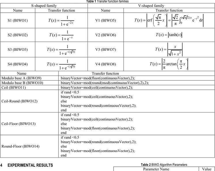
The turbine placement problem is a binary problem, therefore IWO, which has a continuous structure, was converted to a binary form by applying fourteen different transfer functions. The fourteen different methods obtained from the transfer functions were called BIWO1 to BIWO14. From these methods, the method achieving the optimal turbine layout result was renamed BIWO. The transfer functions and methods are shown in Tab. 1 [27-31].

14 different binary IWO algorithms were suggested by using an s-shaped family, a v-shaped family, A, Mod-B, ceil, ceil-floor, ceil-round, round-floor transfer functions. Position vectors were converted into the binary space by using transfer functions to assign values to be 0 or 1. The flowchart for BIWO is shown in Fig. 3 [23, 32].

(4)

Table 1 Transfer function families

S-shaped family V-shaped family

Name Transfer function Name Transfer function

S1 (BIWO1) ( ) 1₂ 1 e x T x = ₋ + V1 (BIWO5) 2 ( π 2) 0 π 2 ( ) erf e d 2 π x _t T x ₌ _ x_ ₌ − t    

∫

S2 (BIWO2) ( ) 1 1 e x T x = ₋ + V2 (BIWO6) T x( ) tanh( )= x S3 (BIWO3) ( ) 1_{( 3)} 1 e x T x = ₋ + V3 (BIWO7) ( ) ₁ 2 x T x x = + S4 (BIWO4) ( ) 1_{( 3)} 1 e x T x = ₋ + V4 (BIWO8) 2 π ( ) arctan π 2 T x = _ x_  

Name Transfer function

Modulo base A (BIWO9) binaryVector=mod(floor(continuousVector),2);

Modulo base B (BIWO10) binaryVector=mod(round(mod(continuousVector),2),2);

Ceil (BIWO11) binaryVector=mod(ceil(continuousVector),2);

Ceil-Round (BIWO12) if rand <0.5 binaryVector=mod(ceil(continuousVector),2); else binaryVector=mod(round(continuousVector),2); end Ceil-Floor (BIWO13) if rand <0.5 binaryVector=mod(ceil(continuousVector),2); else binaryVector=mod(floor(continuousVector),2); end Round-Floor (BIWO14) if rand <0.5 binaryVector=mod(round(continuousVector),2); else binaryVector=mod(floor(continuousVector),2); end 4 EXPERIMENTAL RESULTS

In this study, all results were obtained using the MATLAB 2014(8.3) program. This study was based on published literature data that considered the wind to be unidirectional and moving with a constant velocity of 12 m/s. The wind farm consists of an area of 2000×2000 m. This area was divided into 10×10 and 20×20 square grids. Considering international standards, the distance between the turbines is normally 4 times the diameter (D) [33]. However, some studies used 5D as the distance between turbines, thus it was taken as 5D in this study [12]. Accordingly, the turbines were positioned to make the distance between turbines five times the turbine rotor diameter. A turbine was positioned in the centre of each square to fulfil this requirement. The experimental study was carried out using the BIWO algorithm with a starting population of 50 and a maximum of 1000 iterations. The maximum number of function evaluations was determined to be (MaxFES) 6×105_{similar to other studies in literature.}

These operations were done for the turbine placement problem by independently running the BIWO algorithm ten times. The parameters used in the BIWO algorithm are shown in Tab. 2; the hub height, rotor radius, thrust coefficient and roughness values of the wind turbines are shown in Tab. 3. Using these values, twelve algorithms were applied to the turbine placement problem. The obtained values and the results are shown in Tabs. 4 and 5, respectively.

Table 2 BIWO Algorithm Parameters

Parameter Name Value

Number of Maximum Seeds 5

Number of Minimum Seeds 1

Number of Maximum Population 100

Variance Reduction Coefficient 2

Initial Value of Standard Deviation 0.5

Final Value of Standard Deviation 0.001

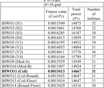
Tab. 4 shows the results obtained by applying fourteen different BIWO algorithms to a 10×10 grid. Examining the results, the s-shaped family functions obtained better fitness values than the v-shaped family functions. The Ceil (BIWO11) algorithm, on the other hand, found the best fitness value among all the algorithms, achieving the highest performance. In addition, hybrid structures (ceil-round (BIWO12), ceil-floor (BIWO13) and (ceil-round-floor (BIWO14)) have obtained fitness values close to the BIWO11 algorithm.

Table 3 Specifications of the wind turbine [14]

Hub height (z, m) 60

Rotor radius (rr, m) 40

Thrust coefficient (CT) 0.88

Terrain roughness (Z0) 0.3

Tab. 5 shows the results obtained by applying fourteen different BIWO algorithms to a 20×20 grid. It was seen that the performance of the v-shaped family algorithms was lower than others. S1 (BIWO1) and Mod-A (BIWO9) algorithms positioned 55 turbines into an area of 2×2 km

(5)

and it was observed that, although the fitness results obtained in the turbine placement operation were close to each other. But the Ceil (BIWO11) algorithm found the best fitness value among all the algorithms, achieving the highest performance. In addition, hybrid structures (ceil-round (BIWO12), ceil-floor (BIWO13) and (ceil-round-floor (BIWO14)) have obtained fitness values close to the BIWO11 algorithm. For this reason, the best results were achieved by the Ceil (BIWO11) algorithm in both grid systems (10×10 and 20×20). In this study, the best placement was achieved by the BIWO11 algorithm using the Ceil transfer function and it was renamed BIWO in the text that follows.

Table 4 shows the results obtained by applying ten different BIWO algorithms to a 10×10 grid 10×10 grid Fitness value (Cost/PT) Total power (PT) Number of turbines BIWO1 (S1) 0.0015549 14875 32 BIWO2 (S2) 0.0015661 14768 32 BIWO3 (S3) 0.0016285 16187 38 BIWO4 (S4) 0.0016413 15059 35 BIWO5 (V1) 0.0016195 14932 34 BIWO6 (V2) 0.0016053 14084 31 BIWO7 (V3) 0.0016011 15776 36 BIWO8 (V4) 0.0016344 15789 37 BIWO9 (Mod-A) 0.0015539 14549 31 BIWO10 (Mod-B) 0.0015497 14924 32 BIWO11 (Ceil) 0.0015413 14667 31 BIWO12 (Ceil-Round) 0.0015435 14647 31 BIWO13 (Ceil-Floor) 0.0015434 14647 31 BIWO14 (Round-Floor) 0.0015429 14316 30

Table 5 shows the results obtained by applying ten different BIWO algorithms to a 20×20 grid 20×20 grid Fitness value (Cost/PT) Total power (PT) Number of turbines BIWO1 (S1) 0.0014595 25187 55 BIWO2 (S2) 0.0015029 25329 57 BIWO3 (S3) 0.0015623 26473 62 BIWO4 (S4) 0.0015953 28002 67 BIWO5 (V1) 0.0015877 27302 65 BIWO6 (V2) 0.0015869 29411 70 BIWO7 (V3) 0.0015676 25963 61 BIWO8 (V4) 0.0015966 27981 67 BIWO9 (Mod-A) 0.0014763 24902 55 BIWO10 (Mod-B) 0.0015102 26512 60 BIWO11 (Ceil) 0.0014149 22382 47 BIWO12 (Ceil-Round) 0.0014437 24567 53 BIWO13 (Ceil-Floor) 0.0014394 23308 50 BIWO14 (Round-Floor) 0.0014376 24670 53

Comparison of the convergence curves of the best fitness values obtained from a 10×10 grid and a 20×20 grid is shown in Fig. 4. This figure indicates that the convergence curve of the proposed algorithm gained stability at approximately the 3500th_generation.

Furthermore, when the turbine farm is represented with a grid structure consisting of more square cells, it is seen that the proposed approach produces better solutions.

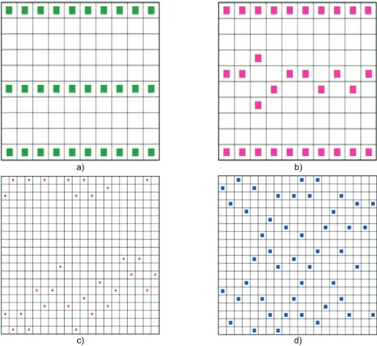
The area, where both 10×10 and 20×20 grids are used, is 2×2 km. The most commonly used grid placement model in the literature is 10×10. However, there has been a study conducted with GA using a 20×20 grid [34]. This study was added to Tab. 6 and 7. In the 10x10 grid, the distance between the grids is 200 m. Therefore, there are a maximum of 100 locations that turbines can be installed. In the 20×20 grid, the distance between the grids is 100 m and there are a maximum of 400 locations that the turbines can be installed. The wake radius is smaller than the size of the 10×10 grid cells. Thus, turbines are positioned in the radial direction and closer together in the 20×20 grid cells [34]. Although the potential positions of turbines in a 20×20 grid are closer to each other, the minimum distance between turbines was protected. Considering a 10×10 grid, the proposed method obtained a better result than the study by Mosetti et al., while it had a closer result to the study by Grady et al. However, comparing the results of a 20×20 grid with those in published literature, it was seen that the proposed method had better performance than studies by Mosetti et al. and Grady et al. in terms of fitness values, revealing a higher success rate. Because a 20×20 grid used the search space more effectively, i.e. the number of independent turbine layouts considerably increased compared to a 10×10 grid, the performance of the BIWO algorithm significantly improved. It was observed in Fig. 5 that a 20×20 grid obtained a more flexible layout than a 10×10 grid. In this study, two grids were used for the wind farm. The first one is the 10×10 grid method consisting of 100 possible locations proposed by Grady et al. The second one is the 20×20 grid method with 400 potential locations suggested in recent studies. Wang et al. reported that using especially a 20×20 grid would give better results [35].

Figure 4 Convergence curves of the BIWO algorithm for distinct grid layout The results of the studies in published literature related the wind turbine placement problem to a 10×10 and 20×20 grid, like the proposed approach, and these are shown in Tab. 6 and 7, respectively.

For a 10×10 grid, the results of the turbine placement problem obtained from Mosetti, Grady and other methods are compared with the proposed method in Tab. 6. The fitness value for the turbine placement operation achieved by the proposed method is 5.09% better than that of Mosetti and 0.15% better than the other approach. In terms of total power, the BIWO method produced more energy than Mosetti did by 18.74% and other methods did by 2.50%. Therefore, according to these results, it was seen that the BIWO method resulted in a better solution for turbine placement in a 10×10 grid.

(6)

Figure 5 Wind farm layouts obtained by (a) Grady, (b) proposed method (10×10) and (c) Parada, (d) proposed method (20×20) Table 6 Comparison of the results obtained for wind farms using 10×10 grid

Method _PowerTotal _AveragePower Number of Turbines Fitness 10−3 GA [10] 12352 475 26 1.6197 GA [11] 14310 477 30 1.5436 MILP [36] 14310 477 30 1.5436 BPSO [14] 14310 477 30 1.5436 Lazy Greedy [16] 14310 477 30 1.5436 GA [34] _(14785)14310 477 30 _(1.4940)1.5436 BIWO (Proposed Method) 14667 473 31 1.5413

For a 20×20 grid, the results of the turbine placement problem obtained from Parada were compared with the proposed method in Tab. 7. No conformity value was found from the comparison of the results with Parada for a 20×20 grid; only the total power values were compared. The proposed method achieved 46.27% more power generation. While BIWO applied to a 20×20 grid performed better than all other methods, it also achieved a very good placement compared to the result of Parada’s study with GA and a 20×20 grid. Considering these results, it can be said that the BIWO is a very good algorithm for the dual turbine placement problem. In Parada’s study, the Gaussian vortex model was used instead of the Jensen vortex model. The values given in parentheses in Tabs. 6 and 7 were obtained using the Gaussian vortex model.

According to the Jensen vortex model, the conformity value obtained seemed to be better due to the difference in the mathematical calculation. When considering 10×10

grids, the conformity value is 0.0015436 for the Jensen grid model and 0.0014940 for the Gaussian grid model. However, these two conformity values were obtained with the same placement, thus, they should be considered equal. For a 20×20 grid, although the conformity value was smaller according to the Gaussian model, BIWO gave a better result.

Table 7 Comparison of the results obtained for wind farms using 20×20 grid Method _PowerTotal _AveragePower Number of

Turbines Fitness 10−3 GA [34] _(15302)-- 510 30 _(1.4390)-- BIWO (Proposed Method) 22382 476 47 1.4149

When we examine both the 10×10 and 20×20 grid systems together, the fitness value for the turbine placement operation achieved by BIWO is 9.1% better than that of Grady. In terms of total power, the BIWO method produced more energy than Grady did by 56.41%. Therefore, according to these results, it was seen that the BIWO method resulted in a better solution for turbine placement.

5 CONCLUSION AND FUTURE WORKS

There are various solution methods for the wind turbine placement. The original IWO is used to solve continuous optimization problems. A new and alternative algorithm (BIWO) was presented to design layouts for an

(7)

efficient wind turbine farm. The model used to calculate the velocity deficiency between the wind turbines is the Jensen-based vortex model. It was seen that the proposed method produced an optimal placement provided that the distance between turbines was constant. The main reason for this is the expansion of the search space where turbines can be placed. In other words, one-square area in a 10×10 grid corresponds to a four-square area in a 20×20 grid. In an area of 2×2 km, there are 100 turbine-areas in a 10×10 grid, while 400 turbines can be placed in a 20×20 grid. That is to say, the BIWO algorithm scanned the search space more effectively. Therefore, the proposed algorithm achieves minimal annual cost for a wind farm by positioning wind turbines with minimum wake loss [37].

At the same time, the distance between the turbines was made to be 5D. The results of the proposed method were compared with those obtained by other methods in published literature.

As a result, the proposed method produced a 9.1% increase in the conformity value, a 56.41% increase in the total power compared to Grady and a 46.27% increase in the total power compared to Parada. This proved BIWO to be an excellent success for the turbine placement problem. The proposed method can be applied to different binary problems in the future, or current algorithms in a modified or hybrid way.

6 REFERENCES

[1] GWEC. (2016). Global Wind Report 2016.

[2] Long, H., Eghlimi, M., & Zhang, Z. (2017). Configuration Optimization and Analysis of a Large Scale PV/Wind System. IEEE Transactions on Sustainable Energy, 8(1), 84-93. https://doi.org/10.1109/TSTE.2016.2583469

[3] Omer, A. M. (2008). Energy, environment and sustainable development. Renewable and sustainable energy reviews,

12(9), 2265-2300. https://doi.org/10.1016/j.rser.2007.05.001

[4] Wang, H. & Huang, J. (2016). Cooperative planning of renewable generations for interconnected microgrids. IEEE

Transactions on Smart Grid, 7(5), 2486-2496.

https://doi.org/10.1109/TSG.2016.2552642 [5] GWEC. (2015). Global Wind Report 2015.

[6] Malen, J. & Marcus, A. A. (2017). Promoting clean energy technology entrepreneurship: The role of external context.

Energy Policy, 102, 7-15.

https://doi.org/10.1016/j.enpol.2016.11.045

[7] Bilgili, M., Şahin, B., & Şimşek, E. (2010). Türkiye’nin güney, güneybatı ve batı bölgelerindeki rüzgar enerjisi potansiyeli. Journal of Thermal Science and Technology,

30(1), 1-12.

[8] Fried, L., Shukla, S., & Sawyer, S. (2012). Global wind

report: annual market update 2011. GWEC.

[9] Holttinen, H. & Ahlgrimm, J. (2013). IEA WIND 2012 Annual Report.

[10] Mosetti, G., Poloni, C., & Diviacco, B. (1994). Optimization of wind turbine positioning in large windfarms by means of a genetic algorithm. Journal of Wind Engineering and

Industrial Aerodynamics, 51(1), 105-116.

https://doi.org/10.1016/0167-6105(94)90080-9

[11] Grady, S., Hussaini, M., & Abdullah, M. M. (2005). Placement of wind turbines using genetic algorithms.

Renewable energy, 30(2), 259-270.

https://doi.org/10.1016/j.renene.2004.05.007

[12] Marmidis, G., Lazarou, S., & Pyrgioti, E. (2008). Optimal placement of wind turbines in a wind park using Monte Carlo simulation. Renewable energy, 33(7), 1455-1460.

[13] González, J. S., Rodriguez, A. G. G., Mora, J. C., Santos, J. R., & Payan, M. B. (2010). Optimization of wind farm turbines layout using an evolutive algorithm. Renewable

energy, 35(8), 1671-1681.

[14] Pookpunt, S. & Ongsakul, W. (2013). Optimal placement of wind turbines within wind farm using binary particle swarm optimization with time-varying acceleration coefficients.

Renewable energy, 55, 266-276.

[15] Wagner, M., Day, J., & Neumann, F. (2013). A fast and effective local search algorithm for optimizing the placement of wind turbines. Renewable energy, 51, 64-70.

[16] Changshui, Z., Guangdong, H., & Jun, W. (2011). A fast algorithm based on the submodular property for optimization of wind turbine positioning. Renewable energy, 36(11), 2951-2958. https://doi.org/10.1016/j.renene.2011.03.045 [17] Shakoor, R., Hassan, M. Y., Raheem, A., & Rasheed, N.

(2015). The modelling of wind farm layout optimization for the reduction of wake losses. Indian Journal of Science and

Technology, 8(17).

https://doi.org/10.17485/ijst/2015/v8i17/69817

[18] Wan, C., Wang, J., Yang, G., Li, X., & Zhang, X. (2009). Optimal micro-siting of wind turbines by genetic algorithms based on improved wind and turbine models. Paper presented at the Decision and Control, 2009 held jointly with the 2009 28th Chinese Control Conference. CDC/CCC 2009.

Proceedings of the 48th_{IEEE Conference on.}

https://doi.org/10.1109/CDC.2009.5399571

[19] Mittal, A. (2010). Optimization of the layout of large wind

farms using a genetic algorithm. (MS), Department of

Mechanical and Aerospace Engineering, Case Western Reserve University.

[20] Massan, S.-u.-R., Wagan, A. I., Shaikh, M. M., & Abro, R. (2015). Wind turbine micrositing by using the firefly algorithm. Applied Soft Computing, 27, 450-456.

https://doi.org/10.1016/j.asoc.2014.09.048

[21] Bharadwaj, V. R. & Siddhartha, G. (2016). Invasive Weed Optimization for Economic Dispatch with Valve Point Effects. Journal of Engineering Science and Technology,

11(2), 237-251.

[22] Mehrabian, A. R. & Lucas, C. (2006). A novel numerical optimization algorithm inspired from weed colonization.

Ecological informatics, 1(4), 355-366.

https://doi.org/10.1016/j.ecoinf.2006.07.003

[23] Ahmed, A., Al-Amin, R., & Amin, R. (2014). Design of static synchronous series compensator based damping controller employing invasive weed optimization algorithm.

SpringerPlus, 3(1), 394.

https://doi.org/10.1186/2193-1801-3-394

[24] Xing, B. & Gao, W.-J. (2014). Invasive weed optimization

algorithm Innovative Computational Intelligence: A Rough Guide to 134 Clever Algorithms : Springer, 177-181.

[25] Zhou, Y., Chen, H., & Zhou, G. (2014). Invasive weed optimization algorithm for optimization no-idle flow shop scheduling problem. Neurocomputing, 137, 285-292. https://doi.org/10.1016/j.neucom.2013.05.063

[26] Roshanaei, M., Lucas, C., & Mehrabian, A. (2009). Adaptive beamforming using a novel numerical optimisation algorithm. IET microwaves, antennas & propagation, 3(5), 765-773. https://doi.org/10.1049/iet-map.2008.0188

[27] Mirjalili, S. & Lewis, A. (2013). S-shaped versus V-shaped transfer functions for binary Particle Swarm Optimization.

Swarm and Evolutionary Computation, 9, 1-14.

https://doi.org/10.1016/j.swevo.2012.09.002

[28] Crawford, B., Soto, R., Olivares-Suárez, M., Palma, W., Paredes, F., Olguin, E., et al. (2014). A binary coded firefly algorithm that solves the set covering problem. Rom. J. Inf.

(8)

[29] Saremi, S., Mirjalili, S., & Lewis, A. (2015). How important is a transfer function in discrete heuristic algorithms. Neural

Computing and Applications, 26(3), 625-640.

https://doi.org/10.1007/s00521-014-1743-5

[30] Koç, İ. (2016). Big Bang-Big Crunch Optimization Algorithm for Solving the Uncapacitated Facility Location Problem. International Journal of Intelligent Systems and

Applications in Engineering, 4(Special Issue-1), 185-189.

https://doi.org/10.18201/ijisae.2016SpecialIssue-146971 [31] Küçükyavuz, S. & Sen, S. (2017). An Introduction to

Two-Stage Stochastic Mixed-Integer Programming. INFORMS

TutORials in Operations Research. https://doi.org/10.1287/educ.2017.0171

[32] Moallem, P. & Razmjooy, N. (2012). A multi layer perceptron neural network trained by invasive weed optimization for potato color image segmentation. Trends in

Applied Sciences Research, 7(6), 445.

https://doi.org/10.3923/tasr.2012.445.455

[33] Pérez, B., Mínguez, R., & Guanche, R. (2013). Offshore wind farm layout optimization using mathematical programming techniques. Renewable energy, 53, 389-399. https://doi.org/10.1016/j.renene.2012.12.007

[34] Parada, L., Herrera, C., Flores, P., & Parada, V. (2017). Wind farm layout optimization using a Gaussian-based wake model. Renewable energy, 107, 531-541.

[35] Wang, L., Tan, A. C., & Gu, Y. (2015). Comparative study on optimizing the wind farm layout using different design methods and cost models. Journal of Wind Engineering and

Industrial Aerodynamics, 146, 1-10.

https://doi.org/10.1016/j.jweia.2015.07.009

[36] Shakoor, R., Hassan, M. Y., Raheem, A., & Rasheed, N. (2016). Wind farm layout optimization using area dimensions and definite point selection techniques.

Renewable energy, 88, 154-163.

[37] Crespo, A., & Herna´ndez, J. (1996). Turbulence characteristics in wind-turbine wakes. Journal of Wind

Engineering and Industrial Aerodynamics, 61(1), 71-85.

https://doi.org/10.1016/0167-6105(95)00033-X Contact information:

Mehmet BEŞKİRLİ, Ph.D. Corresponding author

Department of Computer Engineering, Selçuk University, Konya, Turkey mehmetbes@selcuk.edu.tr İsmail KOÇ, Ph.D.

Department of Computer Engineering, Selçuk University, Konya, Turkey ismailkoc@selcuk.edu.tr Halife KODAZ, Ph.D.

Department of Computer Engineering, Selçuk University, Konya, Turkey hkodaz@selcuk.edu.tr