D O I: 1 0 .1 5 0 1 / C o m m u a 1 _ 0 0 0 0 0 0 0 7 2 3 IS S N 1 3 0 3 –5 9 9 1
MODELING DEPENDENT FINANCIAL ASSETS BY DYNAMIC COPULA AND PORTFOLIO OPTIMIZATION BASED ON CVAR
SIBEL AÇIK KEMALO ¼GLU AND EMEL KIZILOK KARA
Abstract. This paper is concerned with the statistical modeling of the de-pendence structure of multivariate …nancial data using copula. Since …nancial data is greatly a¤ected by the economic factors, it often varies according to the time. Therefore, dynamic copula model is used that takes into account the time-varying. In addition, portfolio optimization based on Mean-CVaR model is applied with Monte Carlo simulation. As an application, a portfolio with four di¤erent Indexes is constructed from the Turkish …nancial markets. The marginal distributions of assets in the portfolio are estimated and parameter estimates are given for the di¤erent copula models. The portfolio optimization based on CVaR is made for the portfolio created from the speci…ed copula model.
1. INTRODUCTION
Modern Portfolio Theory is an approach which had emerged after the 1950s and has enabled the creation of portfolios, taking into account the relationships between assets. Markowitz [1] presented the mean variance model and laid the foundations of modern portfolio theory. Portfolio risk is measured by variance in the mean variance model. When the return data is not distributed normally, it is more appropriate to use other risk measurements instead of measuring risk by variance. Value at Risk (VaR) and Conditional Value at Risk (CVaR) are the most known risk measurements in the …eld of …nance. In the …rst studies carried out in …nance, VaR was used as risk measurement. However, VaR could not ensure the attributes of being subadditive and convex, which are required in a risk measurement. It is of importance to ensure these attributes, particularly in a portfolio optimization. CVaR has been recommended as opposed to VaR, since it can ensure these attributes [2]. In this study, risk measurement was adopted as CVaR, and the mean-CVaR model was used for portfolio optimization.
In order to estimate the portfolio CVaR in a more accurate way, the nonlinear dependency between the tails of return on assets should be revealed. In this study,
Received by the editors: October 21, 2014 Accepted: January 29, 2015. Key words and phrases. Dynamic copula, CVaR, portfolio optimization.
c 2 0 1 5 A n ka ra U n ive rsity 1
the copula model that was …rst mentioned in Sklar [3] was used in order to model the dependency structure between the return series. However, since the …nancial data exploited varied with respect to time, the dynamic copula model was applied to the data instead of a known copula model [4].
In order to conduct a portfolio optimization based on CVaR , the copula para-meter should primarily be estimated. In the literature, there are di¤erent methods for the copula parameter estimation. The Inference Function for Margins (IFM) method, based on the marginal distribution, Kendall’s based on sequence inde-pendent of marginal functions and Maximum Pseudo Likelihood (MPL) method, are the most known estimation methods. In this study, Two-Stage IFM method was used. In this method, the parameter of marginal distribution is estimated in the …rst phase, and copula parameter is estimated in the second phase [5]. For the test of marginal and copula goodness of …t, AIC and BIC criteria were applied. Finally, portfolio optimization based on the CVaR risk measurement was made for the data generated from this model with the Monte Carlo simulation method, and the weights in the portfolio were determined.
Comprehensive information regarding copula is available in the study of Joe [6] and Nelsen [7].
In the …eld of …nance, copula was …rst mentioned by Embrechts et al. [8]. The …rst applications of this subject were given in Cherubini [5]. Jondeau and Rockinger [9] used the Copula-GARCH model in order to determine the dependence structure among stocks. Other studies that included this model have been presented in Wei and Zhang [10], Ozun and Cifter [11], and Huang et al. [12]. Optimization studies based on CVaR were recommended in Uryasev and Rockafellar [2] for the …rst time. The application of the copula-GARCH model for portfolio risk analysis was given in Wu and Chen [13], and Wang et al. [14]. He and Li [4] have conducted studies regarding the dynamic copula model based on CVaR and copula.
In the second part of the study, the dynamic copula model is introduced, and methods to …nd the estimations for parameters are given. In the third part, the de…nition of CVaR risk measurement is presented nd portfolio optimization based on CVaR is formed. In the fourth part, for a sample of Turkish …nancial data is tested and the results are presented. Finally, in the …fth part, the results are discussed and further studies that could be conducted in the future are mentioned.
2. DYNAMIC COPULA MODEL AND PARAMETER ESTIMATION Copula functions are frequently used in modeling the dependency structure among the risk variables in the …eld of …nance and actuary. Sklar [3] states that there is only one expression of an n-dimensional C( ; : : : ) copula for any continuous (X1; :::; Xn) random vector:
where F1( ) ; :::; FN( ) and F ( ; :::; ) respectively show the marginal and joint dis-tribution functions of x1; x2; :::; xn random variables.
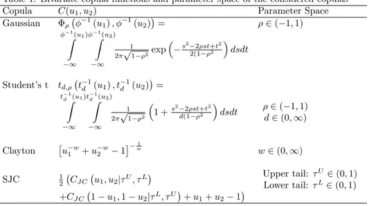
In this study, static copula models (Gaussian, Student-t, Clayton, and Sym-metrized Joe Clayton-SJC) and corresponding dynamic copula models (GDCC, tDCC, tvC, tvSJC) are used. The static copulas exploited are de…ned as follows [5, 7, 15]
Table 1. Bivariate copula functions and parameter space of the considered copulas
Copula C(u1; u2) Parameter Space
Gaussian 1(u1) ; 1(u2) = 2 ( 1; 1) 1(u 1) Z 1 1(u 2) Z 1 1 2 p1 2exp s2 2 st+t2 2(1 2 dsdt Student’s t td; td1(u1) ; td1(u2) = tdZ1(u1) 1 tdZ1(u2) 1 1 2 p1 2 1 + s2 2 st+t2 d(1 2 dsdt 2 ( 1; 1) d 2 (0; 1) Clayton u w 1 + u2w 1 1 w w 2 (0; 1) SJC 1 2 CJ C u1; u2j U; L Upper tail: U2 (0; 1) Lower tail: L2 (0; 1) +CJ C 1 u1; 1 u2j L; U + u1+ u2 1
A lso note that 1and t 1
d are the inverse of the N orm al and t-student c.d.f., w here the param eters
and d are the co e¢ cient of linear correlation and the degrees of freedom , resp ectively. Jo e-C layton copula is de…ned as CJ C u1; u2j U; L = 1 1 [1 (1 u1) ] + [1 1 u/2 ] 1 1= 1= ; w here = 1 log2(2 U )and = 1 log2( L)
The used dynamic copula are created by applying the static copulas which are de…ned in Table 1. According to the Sklar [3] theorem, the dynamic copula model is expressed as below [11].
F (X1t; :::; Xntj t) = Ct(F1t(X1tj t) ; F2t(X2t j t) :::; Fnt(Xntj t)) (2.2) where t= fX1t 1; X2t 2; :::; Xnt t; :::g for t = 1; 2; :::; T represents the historical data until t time.
The …rst step to create the joint distribution of portfolio assets with the dynamic copula method is generating the marginal distribution of each asset. In the litera-ture, since the …nancial data varies according to the time, it is stated that marginal distributions are in compliance with the GARCH model, which was …rst run by Bollerslev [16]. The GJR model was acquired by adding the dummy variable to the GARCH model.
GARCH(1; 1) n and GARCH(1; 1) t models can be expressed as below: xt = + at (2.3) at = t"t 2 t = 0+ 1a2t 1+ 2t 1 "t N (0; 1) or "t td
Here, provided that indicates conditional mean of return series, and 2 t 1 indicates conditional variance, it is de…ned as below. Moreover, t 1indicates the information set and d indicates the degree of freedom.
= E (xt) = E (E (xtj t 1)) = E ( t) = 2
t = V ar (xtj t 1) = V ar (atj t 1) 0 > 0; 1 0; 0 ve 1+ < 1 GJR-n and GJR- t models are de…ned as:
xt = + at (2.4) at = t"t 2 t = 0+ 1a2t 1+ 2t 1+ st 1a2t 1 "t N (0; 1) or "t td where,st 1= 1; at 1< 0
0; at 1 0 is a dummy variable which is equal to 0 as opposed to 1 while "tis negative. Moreover, parameter intervals are given as 0> 0; 1 0; 0 , + 0 and 1+ +12 < 1.
The parameters of the GARCH and GJR models are estimated with MLE method. The joint density function can be expressed as
f (a1; :::; at) = f (atj t 1) f (at 1j t 2) :::f (a1j 0) f (a0)
where t 1= fa0; a1; :::; at 1g : Given data a1; :::; at, the log-likelihood function is given as: LL = n 1 X k=0 f (an kj n k 1)
Here, the conditional marginal distribution of Xt+1for the GARCH(1; 1) model is de…ned as follows: P (Xt+1 xj t) = P (at+1 (x ) j t) = P "t+1 (x ) p 0+ 1a2t+ 2t j t ! 8 > > < > > : N p (x ) 0+ 1a2t+ 2tj t ; " N (0; 1) td p (x ) 0+ 1a2t+ 2tj t ; " td
For the GJ R(1; 1) model: P (Xt+1 xj t) = P (at+1 (x ) j t) = P "t+1 (x ) p 0+ 1a2t+ 2t+ sta2t j t ! 8 > > < > > : N p (x ) 0+ 1a2t+ 2t+ sta2tj t ; " N (0; 1) td p (x ) 0+ 1a2t+ 2t+ sta2tj t ; " td
The copula parameter should also be estimated in order to conduct portfolio optimization based on CVaR. Therefore, the IFM method that is composed of two phases based on the method of Maximum Likelihood Estimation (MLE) was used. The IFM estimates the marginal distribution parameters separately from the copula parameters. The estimation procedure of the IFM method consists of two steps [5].
In the …rst step, the parameters of the marginals are estimated: b1= arg max 1 T X t=1 n X j=1 ln fj(xjt; 1) : (2.5)
In the second step, the parameter of the copula model is estimated, given 1: b2= arg max 2
T X t=1
ln c F1(x1t) ; F2(x2t) ; :::; Fn(xnt) ; 2; b1 : (2.6) The IFM estimator is de…ned as(Cherubini et.al.,[5])
bIF M = b1; b2 0
(2.7) To make the goodness of …t tests for marginal and copula, AIC (Akaike Infor-mation Criterion) [17] and BIC (Bayesian InforInfor-mation Criterion) [18, 19] criteria were used. AIC and BIC values are,
AIC = 2 LL + 2k (2.8)
BIC = 2 LL + ln(n) k (2.9)
where LL is the log-likelihood at its maximum point of the model estimated and k is the number of copula parameters in the model. According to these criteria, the best choice is the model with minimum AIC or BIC value.
3. PORTFOLIO OPTIMIZATION BASED ON CVAR
CVaR measurement was introduced to the literature by the development of VaR measurement by Rockafellar and Uryasev [2]. Let x = (x1; x2; :::; xn)T vector be a
portfolio with n assets, and let y = (y1; y2; :::; ym)T be m type loss factor with p(y) density distribution. The loss factor of portfolio f (x; y) is given as follows:
(x; ) = Z
f (x;y)
p(y)dy; 2 R
For the given 2 (0; 1) con…dence level
(x) = min f 2 R : (x; ) g (x) = E [f (x; y)jf(x; y) (x)] = 1 1 Z f (x;y) (x) f (x; y)p(y)dy
(x) and (x) show V aR and CV aR at con…dence level, respectively. Rock-afellar and Uryasev [2] converted the minimization problem of CV aR to that of F (x; ) . Here, F (x; ) is a constantly di¤erentiable function, which is composed of convex composition of V aR and CV aR.
F (x; ) = + 1
1 Z
y2Rm
[f (x; y) ]+p(y)dy (3.1)
Since the analytical expression of p(y) is di¢ cult, or it is not known generally in practice, y’s are derived through the Monte Carlo simulation method. Accordingly, the (3.1) equation can be written as follows:
e F (x; ) = + 1 m (1 ) m X j=1 xTyj + (3.2) Here, provided that m indicates the number of simulations, x = (x1; x2; :::; xn) indicates the weights of assets in the portfolio, and yj = (yj1; yj2; :::; yjn) indicates the derived returns, the portfolio selection model based on CV aR optimization is given as below: min eF (x; ) = + 1 m (1 ) m X j=1 zj zj = xTyj + 8 > > > > > < > > > > > : xTy j+ + zj 0 zj 0 1 qx T m X j=1 yj Pm i=1xi= 1; x 0 9 > > > > > = > > > > > ; (3.3)
Here, is the return expected by investor. CV aR optimization problem can be solved as a linear programming problem. Returns generated from the dynamic copula model are obtained from the Monte Carlo simulation.
4. NUMERICAL EXAMPLE
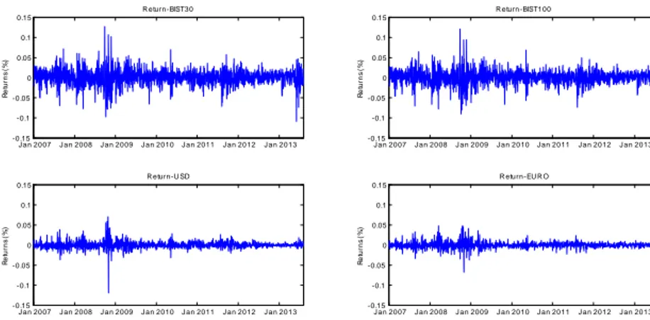
In this study, in order to demonstrate the performance of the copula-GARCH model, 1649 daily stock …nal quotations between January 4, 2007 and August 1, 2013, as well as USD and EURO currency data, were used. Stock …nal quotations were obtained from the website of BIST [20], and USD and EURO currency data were retrieved from the website of the Turkish Central Bank [21]. Daily market returns of BIST30, BIST100, USD and EURO are shown in Figure 1.
When rt indicates the returns, it is given as:
rt= 100 ln Pt Pt 1
Here Ptindicates the index value at t time. The existence of volatility clustering is seen in Figure 1. Therefore, the results are given in Table 2, after quadratic returns that are named as ARCH e¤ects are tested with the Engle test (LM(4), LM(6), LM(8), and LM(10)) to reveal whether there is a relation to the series.
J an 2007 J an 2008J an 2009 J an 2010 J an 2011 J an 2012 J an 2013 -0 .15 -0.1 -0 .05 0 0.05 0.1 0.15 R et ur ns ( % ) R eturn-BIST30 J an 2007 J an 2008 J an 2009 J an 2010J an 2011 J an 2012 J an 2013 -0 .15 -0.1 -0 .05 0 0.05 0.1 0.15 R et ur ns ( % ) R eturn -BIST100 J an 2007 J an 2008J an 2009 J an 2010 J an 2011 J an 2012 J an 2013 -0 .15 -0.1 -0 .05 0 0.05 0.1 0.15 R et ur ns ( % ) R eturn-U SD J an 2007 J an 2008 J an 2009 J an 2010J an 2011 J an 2012 J an 2013 -0 .15 -0.1 -0 .05 0 0.05 0.1 0.15 R et ur ns ( % ) R eturn-EU R O
0 5 10 15 20 -0.2
0 0.2
Lag
Sample Autocorrelation Functions (ACF)
0 5 10 15 20
-0.2 0 0.2
Lag
Sample Partial Autocorrelation Functions (PACF)
Sa m p le Pa rtia l A u to co rr ela ti o n s 0 5 10 15 20 -0.2 0 0.2 Lag S am p le Au to co rr el at io n s BIST30 0 5 10 15 20 -0.2 0 0.2 Lag BIST100 0 5 10 15 20 -0.2 0 0.2 Lag USD 0 5 10 15 20 -0.2 0 0.2 Lag USD 0 5 10 15 20 -0.2 0 0.2 Lag EURO 0 5 10 15 20 -0.2 0 0.2 Lag EURO (a) (b) BIST30 BIST100
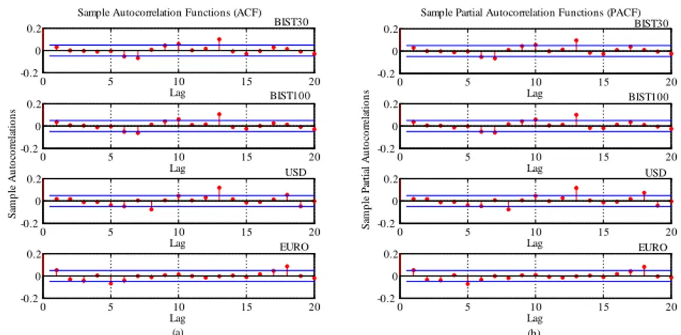
Figure 2. Autocorrelations of BIST30, BIST100, USD and EURO indexes (a) and partial autocorrelation measurements (b)
Table 2. Descriptive statistics and tests
Statistics BIST30 BIST100 USD EURO
Sample Number 1646 1646 1646 1646
Mean 0.000462 0.000479 0.000191 0.000195
Standart deviation 0.0200 0.0185 0.0090 0.0081
Skewness -0.1174 -0.2545 -0.5112 0.2224
Kurtosis 3.7106 4.1608 24.03122 7.4139
Tests Q-stat p-value Q-stat p-value Q-stat p-value Q-stat p-value Jarque-Bera 940.51 0.0010 1195.9 0.0010 39427 0.0010 3756.8 0.0010 LM(4) 118.5178 0.0000 124.0513 0.0000 227.9964 0.0000 191.0501 0.0000 LM(6) 129.5706 0.0000 132.7788 0.0000 228.3458 0.0000 199.3508 0.0000 LM(8) 160.8098 0.0000 152.2154 0.0000 286.3049 0.0000 258.9005 0.0000 LM(10) 166.1320 0.0000 155.6451 0.0000 287.7057 0.0000 268.2120 0.0000
Table 2 consists of summary statistics of …nancial returns and statistical test information in relation to ARCH e¤ects. Thus, it is revealed that BIST30, BIST100, and USD have negative skewness (-0.1174, -0.2545 and -0.5112, respectively), the EURO has a positive skewness (0.2224), and marginal are not distributed normally according to JB statistics (p value < 0:05). It should be looked to the Engle test results to determine whether there is correlation between the data related to each …nancial return. According to the Engle test results, LM statistics indicate that there are ARCH e¤ects (p value < 0:05). Furthermore, the correlations for raw returns in Figure 2 were evaluated with autocorrelation functions (ACF) and partial autocorrelation functions (PACF). Here, it was observed that all autocorrelations are not zero after zero lag. Since …nancial returns are considered to be time series data, their marginal distributions were regarded as GARCH and GJR models to conduct copula estimation. Another result that supports the selection of these
models is that kurtosis coe¢ cients that were computed for each of the …nancial returns were found to be greater than 3. As a consequence, empiric observations in regard to returns have greater leptokurtosis than the normal distribution. Goodness of …t for the distribution with regard to the residual series of each of the …nancial returns (BIST30, BIST100, USD, and EURO) were made for the GARCH and GJR models by selecting Normal and Student-t, respectively.
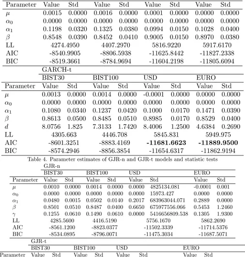
Table 3 and Table 4 respectively show maximum likelihood results, estimated parameter values, AIC (Akaike Information Criterion) and BIC (Bayesian Informa-tion Criterion) values for GARCH and GJR models selecInforma-tion.
In order to determine the model that best explains …nancial returns, minimum AIC and BIC values should be sought in the tables. Table 3 and Table 4 demon-strate that the GJR-t (AIC:-8612.8174,-8895.0195) model can be used for BIST 30 and BIST 100, and the GARCH-t (AIC: -11681.6623, -11889.9500) model can be used for USD and EURO.
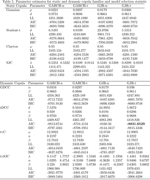
An appropriate copula model was selected by using the estimated parameter val-ues for the identi…ed marginal distributions. Four copula functions were created for the application. The copula selection model was examined in two situations: static (Gaussian, Student-t, Clayton, SJC) and dynamic (GDCC, tDCC, tvC, tvSJC). Table 5 demonstrates the parameter estimation results for the IFM method in re-gard to these situations, and AIC and BIC values. From the table, it is understood that in both situations, the Student-t copula is the best copula model in order to explain the dependency structure of …nancial returns with four variables. When examined separately for static and dynamic situations, the dependency structure of GJR marginal distributions with the minimum AIC (-8831.6529) in a dynamic situation was modeled ideally with tDCC copula.
It was identi…ed that …nancial data marginals that were used …t GJR-t, and joint dependency structure …t the tDCC dynamic copula model. By using the parameter values for selected model, the Monte Carlo simulation was performed 10,000 times, and portfolio optimization was achieved based on CVaR risk measurement. VaR and CVaR risk measurement values for di¤erent con…dence levels, and results in-cluding the weights for each …nancial asset are given in Table 6. Accordingly, mean loss above a certain value, that is, CVAR value would reach the minimum when an investor allocates 35% of his/her assets in BIST30, 15% in BIST100, 30% in USD, and 20% in EURO within a 99% con…dence level.
Table 3. Parameter estimates of GARCH-n and GARCH-t models and statistic tests GARCH-n
BIST30 BIST100 USD EURO
Parameter Value Std Value Std Value Std Value Std
0.0015 0.0000 0.0016 0.0000 0.0001 0.0000 0.0000 0.0000 0 0.0000 0.0000 0.0000 0.0000 0.0000 0.0000 0.0000 0.0000 1 0.1198 0.0320 0.1325 0.0380 0.0994 0.0150 0.1028 0.0400 0.8548 0.0390 0.8452 0.0410 0.9005 0.0150 0.8970 0.0380 LL 4274.4950 4407.2970 5816.9220 5917.6170 AIC -8540.9905 -8806.5938 -11625.8442 -11827.2338 BIC -8519.3661 -8784.9694 -11604.2198 -11805.6094 GARCH-t
BIST30 BIST100 USD EURO
Parameter Value Std Value Std Value Std Value Std
0.0013 0.0000 0.0014 0.0000 -0.0001 0.0000 0.0000 0.0000 0 0.0000 0.0000 0.0000 0.0000 0.0000 0.0000 0.0000 0.0000 1 0.1080 0.0340 0.1237 0.0420 0.1000 0.0170 0.1471 0.0390 0.8613 0.0500 0.8485 0.0510 0.8985 0.0170 0.8529 0.0400 d 8.0756 1.825 7.3133 1.7420 8.4006 1.2500 4.6384 0.2690 LL 4305.663 4446.708 5845.831 5949.975 AIC -8601.3251 -8883.4169 -11681.6623 -11889.9500 BIC -8574.2946 -8856.3854 -11654.6317 -11862.9194
Table 4. Parameter estimates of GJR-n and GJR-t models and statistic tests GJR-n
BIST30 BIST100 USD EURO
Parameter Value Std Value Std Value Std Value Std
0.0010 0.0000 0.0014 0.0000 0.0000 4825134.081 -0.0001 0.001 0 0.0000 0.0000 0.0000 0.0000 0.0000 15973.427 0.0000 0.0000 1 0.0480 0.0015 0.0502 0.0140 0.2017 683963044.071 0.2889 0.0000 0.8501 0.0510 0.8487 0.0400 0.6650 675977556.066 0.5453 1.2460 0.1255 0.0610 0.1490 0.0610 0.0000 5416656809.538 0.1305 1.9300 LL 4285.5600 4416.5190 5756.1670 5862.2690 AIC -8561.1200 -8823.0377 -11502.3339 -11714.5376 BIC -8534.0895 -8796.0071 -11475.3034 -11687.5071 GJR-t
BIST30 BIST100 USD EURO
Parameter Value Std Value Std Value Std Value Std
0.0010 0.0000 0.0011 0.0000 -0.0002 1406475.109 0.0000 28078131.946 0 0.0000 0.0000 0.0000 0.0000 0.0000 8879.443 0.0000 221202.851 1 0.0532 0.0170 0.0618 0.0180 0.3678 276992226.475 0.2539 29560250106.651 0.8371 0.0700 0.8198 0.0610 0.6226 426936136.846 0.7147 2212994007.407 0.1294 0.0800 0.1291 0.0660 0.0000 2473886510.168 0.0003 47746730949.042 d 7.9437 1.5840 7.2247 1.2100 5.2103 5946045507.02 3.9473 13182520678.426 LL 4312.1270 4453.5100 5810.7600 5937.0560 AIC -8612.2540 -8895.0195 -11609.5192 -11862.1122 BIC -8579.8174 -8862.5829 -11577.0826 -11829.6756
Table 5. Parameter estimates for static and dynamic copula families and model selection statistic Static Copula Parameter GARCH-n GARCH-t GJR-n GJR-t
Gaussian 0.0221 0.0297 0.0179 0.0360 d 0.9731 0.9686 0.9664 0.9611 LL 4351.2600 4329.1890 4055.8200 4347.8940 AIC -8704.5208 -8654.3780 -8107.6392 -8691.7872 BIC -8693.7086 -8643.5658 -8096.8270 -8680.9750 Student-t d 6.5491 8.0109 23.9706 5.5313 LL 4290.433 4243.688 3981.715 4330.352 AIC -8578.8664 -8485.9692 -7961.4291 -8658.7042 BIC -8573.4603 -8479.9692 -7956.0230 -8653.2981 Clayton ! 0.85 0.85 0.85 0.85 LL 3103.124 3103.277 2833.643 3101.575 AIC -6204.2483 -6204.5538 -5665.2859 -6201.1500 BIC -6198.8422 -6199.1477 -5659.8798 -6195.7439 SJC 0.5353 0.5322 0.8109 0.8144 0.5348 0.5388 0.8299 0.8319 LL 1413.471 2299.055 1443.225 2424.352 AIC -2822.9424 -4594.1105 -2882.4507 -4844.7030 BIC -2812.1302 -4583.2983 -2871.6385 -4833.8908
Dynamic Copula Parameter GARCH-n GARCH-t GJR-n GJR-t
GDCC 0.0316 0.0297 0.0179 0.036 0.9663 0.9686 0.9663 0.9611 LL 4358.363 4329.189 4055.820 4347.894 AIC -8712.7252 -8654.3780 -8107.6391 -8691.7870 BIC -8701.9130 -8643.5658 -8096.8269 -8680.9748 tDCC d 7.5376 9.5010 24.9955 5.9672 0.028 0.0266 0.0194 0.0286 0.9703 0.9718 0.9684 0.9688 LL 4409.837 4365.207 4083.280 4418.826 AIC -8813.6744 -8724.4134 -8160.56 -8831.6529 BIC -8797.4561 -8708.1951 -8144.3417 -8815.4346 tvC ! 12.8923 12.8913 12.8748 12.8905 0.2197 0.2223 0.2343 0.2222 12.7842 12.7839 12.704 12.7857 LL 2430.023 2433.630 2403.856 2423.371 AIC -4854.0459 -4861.2597 -4801.7120 -4840.7423 BIC -4837.8276 -4845.0414 -4785.4937 -4824.5240 tvSJC 9.1147 1.7757 -2.3995 1.5160 -0.4491 1.1956 1.4481 9.9382 1.0295 8.4754 -8.3109 7.6800 -0.3626 1.2357 9.9486 9.6797 3.228 3.9021 2.9388 5.0730 -0.4471 -0,3567 2.6305 3.0602 LL 1966.988 1706.809 1431.022 1976.633 AIC -3921.9770 -3401.6179 -2850.0436 -3941.2664 BIC -3889.5404 -3369.1812 -2817.6070 -3908.8298
Table 6. The results of portfolio optimization based on CVaR
V aR CV aR x1 BIST30 x2 BIST100 x3 USD x4 EURO
90% 0.0057 0.0102 0.3888 0.1552 0.2676 0.1884
95% 0.0084 0.0136 0.3760 0.1611 0.2715 0.1913
5. CONCLUSION AND DISCUSSION
In this study, the dynamic Copula model was introduced and applied to four di¤erent sets of …nancial data (BIST30, BIST100, USD, EURO) in Turkey. In order to shape the model, …rst, the marginal distributions of the data series were determined as GJR-t, and by using identi…ed marginal distributions, the copula model that established the dependency structure between the data series was se-lected as dynamic t (tDCC). By conducting the simulation, portfolio optimization was achieved based on CVaR risk measurement. Therefore, it can be inferred that investment in BIST30 is the best at each con…dential level in accordance with the portfolio optimization results based on the minimization of CVaR. Other best in-vestments are USD, EURO, and BIST100 respectively.
It is possible to add extreme value theory to the model due to the fat tail of …nancial data. Another possibility is to take into account the change points; we can o¤er di¤erent models for every period. Those will be topics of the future work.
References
[1] Markowitz, H. (1952) ‘Portfolio Selection. Journal of Finance’, vol. 25, pp. 77-91.
[2] Rockafellar, R. T. and Ursayev, S. (2002) ‘Optimization of conditional value at risk’, Journal of Risk, vol. 2, pp. 21-40.
[3] Sklar, A. (1959) ‘Functions De Repartition An Dimensions At Leurs Marges’, Publications De L’¬nstitut De Statistique De L’université De Paris, vol. 8, pp. 229-231.
[4] He, H. and Li, P. (2011) ‘Dynamic Asset Allocation Based on Copula and CVaR’, IEEE. [5] Cherubini, U., Luciano, E. and Vecchiato, W. (2004) Copula Methods in Finance. John Wiley
and Sons, New York.
[6] Joe, H.and Xu, J.J. (1996) The estimation method of inference functions for margins for multivariate models. Technical Report 166. Department of Statistics, University of British Columbia.
[7] Nelsen, R.B. (2006) An Introduction to Copulas, (second ed) Springer, New York.
[8] Emrechts, P., McNeil, A. and Straumann D. (2002). ‘Correlation and dependence in risk management: properties and pitfalls’, In Risk Management Value at Risk and Beyond (Edited by M. Dempster), pp. 176-223, Cambridge University Press.
[9] Rockinger, M. and Jondeau, E. (2006) ‘The Coplua-GARCH model of conditional dependen-cies: An international stock market application’, Journal of International Money and Finance, vol. 25(3), pp. 827-853.
[10] Wei, Y. and Zhang, S. (2007) ‘Multivariate Copula-GARCH Model and Its Applications in Financial Risk Analysis [J].’, Application of Statistics and Management,vol. 3, pp. 008. [11] Ozun, A., Cifter, A. (2007) ‘Portfolio value-at-risk with time-varying copula: Evidence from
the Americans’, Marmara University. MPRA Paper No. 2711.
[12] Huang, J. J., Lee, K. J., Liang, H. and Lin, W.F. (2009) ‘Estimating value at risk of portfolio by conditional copula-GARCH method’, Insurance: Mathematics and Economics, vol. 45, pp. 315- 324.
[13] Wu, Z.X., Chen, M. and Ye, W.Y. (2006) ‘Risk Analysis of Portfolio by Copula-GARCH’, Journal of Systems Engineering Theory and Practice, vol. 2(8), pp. 45–52.
[14] Wang, Z. R., Chen, X. H., Jin, Y. B., Zhou, Y.J. (2010) ‘Estimating risk of foreign exchange portfolio: Using VaR and CVaR based on GARCH-EVT-Copula model’, Physica A, vol. 389, pp. 4918-4928.
[15] Patton, A.J. (2006) ‘Modelling asymmetric exchange rate dependence’, International Eco-nomic Review, vol. 47, pp. 527-556.
[16] Bollerslev, T. (1986) ‘Generalized autoregressive conditional heteroskedasticity’, Journal of econometrics, vol. 31 (3), pp. 307-327.
[17] Akaike, H. (1974) ‘A new look at the statistical model identi…cation’, Automatic Control, IEEE Transactions on, vol. 19, pp. 716–723.
[18] Schwarz, G. (1978) ‘Estimating the dimension of a model’, Annals of Statistics, vol. 6, pp. 461–464.
[19] Cryer, C.D. and Chan, K.S. (2008). Time Series Analysis with Applications in R, (second ed.) Springer, New York.
[20] http://borsaistanbul.com/veriler/verileralt/hisse-senetleri-piyasasi-verileri/endeks-verileri [02.08.2013].
[21] http://evds.tcmb.gov.tr/cbt.html [02.08.2013].
Address : Ankara University, Faculty of Sciences, Department. of Statistics, Ankara, Kirikkale University, Faculty of Arts and Sciences, Department of Actuarial Science, Kirikkale, TURKEY
E-mail : [email protected], [email protected]
0Ba¸sl¬k:Ba¼g¬ml¬ …nansal varl¬klar¬n dinamik ba¼g ve CVaR’a dayal¬ portföy optimizasyonu ile
modellenmesi