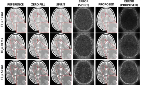
Rapid multi-contrast magnetic resonance imaging and time-of-flight angiography
Tam metin
Şekil


Benzer Belgeler
İnsan serviks kanseri hücre hattında yapılan bir çalışmada; 50µM genistein ile muamele edilen kanserli hücrelerde, HDAC enzim aktivitesinin ve HMT
Gıda endüstrinin gelişmesi, hızlı kentleşmenin sonucunda ev dışında yemek yeme zorunda olan kişilerin tercihleri, kadının iş hayatına atılması sebebiyle yemek
Tablo 3.3: D-Glukozun spektrum eşleştirme yöntemi için kullanılan deneysel- hesapsal özgün absorpsiyon bantları (DF ve TF), absorbans değerleri (DA ve TA)
Until we have demonstrated efficient frequency upconversion using an optical parametric oscillator pumped by a femtosecond Ti:sapphire laser that employ a single
Micro milling experiments were performed on each sample and process outputs such as cutting forces, areal surface texture, built-up edge (BUE) formation, and alterations in
While a few results have been reported on counting series of unlabeled bipartite graphs [ 1 – 4 ], no closed-form expression is known for the exact number of such graphs in
Pamela Bowell, Brian Heap (Bowell & Heap, 2001), this study focuses on parallel elements between Cecily O’Neill’s process drama structures, based on her definition given
AÇILIŞ KONSERİ/OPENING CONCERT CLUJ-NAPOCA FİLARMONİ ORKESTRASI CLUJ-NAPOCA PHILARMONY ORCHESTRA 20.6.1984 Atatürk Kültür Merkezi 21.30 Şef/Conductor: Cristian
