Solution of electromagnetics problems with the equivalence principle algorithm

(1)

SOLUTION OF ELECTROMAGNETICS

PROBLEMS WITH THE EQUIVALENCE

PRINCIPLE ALGORITHM

a thesis

submitted to the department of electrical and

electronics engineering

and the institute of engineering and science

of bilkent university

in partial fulfillment of the requirements

for the degree of

master of science

By

Burak Tiryaki

September 2010

(2)

I certify that I have read this thesis and that in my opinion it is fully adequate, in scope and in quality, as a thesis for the degree of Master of Science.

Prof. Dr. Levent G¨urel (Supervisor)

Prof. Dr. Feza Arıkan

Assoc. Prof. Vakur B. Ert¨urk

Approved for the Institute of Engineering and Sciences:

Prof. Dr. Levent Onural

(3)

ABSTRACT

SOLUTION OF ELECTROMAGNETICS

PROBLEMS WITH THE EQUIVALENCE

PRINCIPLE ALGORITHM

Burak Tiryaki

M.S. in Electrical and Electronics Engineering

Supervisor: Prof. Dr. Levent G¨

urel

September 2010

A domain decomposition scheme based on the equivalence principle for integral equations is studied. This thesis discusses the application of the equivalence principle algorithm (EPA) in solving electromagnetics scattering problems by multiple three-dimensional perfect electric conductor (PEC) objects of arbitrary shapes. The main advantage of EPA is to improve the condition number of the system matrix. This is very important when the matrix equation is solved itera-tively, e.g., with Krylov subspace methods. EPA starts solving electromagnetics problems by separating a large complex structure into basic parts, which may consist of one or more objects with arbitrary shapes. Each one is enclosed by an equivalence surface (ES). Then, the surface equivalence principle operator is used to calculate scattering via equivalent surface, and radiation from one ES to an other can be captured using the translation operators. EPA loses its accuracy if ESs are very close to each other, or if an ES is very close to PEC object. As a remedy of this problem, tangential-EPA (T-EPA) is introduced. Properties of both algorithms are investigated and discussed in detail. Accuracy and the eﬃciency of the methods are compared to those of the multilevel fast multipole

(4)

algorithm.

Keywords: Equivalence principle algorithm, electromagnetic scattering, domain

decomposition method, iterative solution, equivalence principle, method of mo-ments (MoM), Huygens’ principle.

(5)

¨

OZET

ELEKTROMANYET˙IK PROBLEMLER˙IN ES

¸DE ˘

GERL˙IK

PRENS˙IB˙I Y ¨

ONTEM˙IYLE C

¸ ¨

OZ ¨

UMLER˙I

Burak Tiryaki

Elektrik ve Elektronik M¨

uhendisli˘

gi B¨

ol¨

um¨

u Y¨

uksek Lisans

Tez Y¨

oneticisi: Prof. Dr. Levent G¨

urel

Eyl¨

ul 2010

Geli¸sigüzel ¸sekilli ü¸c boyutlu iletken yüzeyleri i¸ceren elektromanyetik sa¸cılım problemlerinin ¸cözümü i¸cin e¸sde˘gerlik prensibi algoritması (EPA) yöntemi

in-celenmi¸stir. EPA y¨ontemi ile elde edilen sistem matrisi, momentler metodu ve

hızlı ¸cok kutup y¨ontemleri gibi geleneksel y¨ontemlerle elde edilen sistem

matri-sine kısayla ¸cok daha iyi ko¸sullu olmaktadır. Bu da, EPA’nın en b¨uy¨uk

avantaj-larından birisidir. Bunun ¨onemi, sistem matrisinin Krylov alt uzay y¨ontemleriyle

iteratif olarak ¸cözümünde ortaya ¸cıkmaktadır. EPA elektromanyetik

problem-lerin ¸cözümüne, büyük ve karma¸sık geometrileri kü¸cük ve basit geometrilere

ayırarak ba¸slar. Elde edilen yeni alt problemlerin her biri e¸sde˘ger y¨uzeylerle

¸cevrelenirler. E¸sde˘ger yüzeylerden meydana gelen sa¸cılım e¸sde˘gerlik prensibi operatörleri kullanılarak, e¸sde˘ger yüzeyler arasındakı etkile¸simler ise öteleme

operat¨orleri kullanılarak hesaplanmaktadır. E¸sde˘ger y¨uzeyler arasındaki veya

e¸sde˘ger y¨uzeyle metal cisim arasındaki mesafenin ¸cok az olması durumunda EPA

ile yapılan ¸cözümün do˘grulu˘gu azalmaktadır. Bu soruna ¸cözüm olarak te˘getsel

EPA (T-EPA) y¨ontemi kullanılmı¸stır. Bu tezde, EPA ve T-EPA’nın ¨ozellikleri

incelenecek ve detaylı bir ¸sekilde tartı¸sılacaktır. Y¨ontemin do˘grulu˘gu ve ver-imlili˘gi ¸cok seviyeli hızlı ¸cok kutup y¨ontemiyle kar¸sıla¸stırılacaktır.

(6)

Anahtar kelimeler: E¸sde˘gerlik prensibi algoritması, elektromanyetik sa¸cılım, it-erative ¸cözücüler, e¸sde˘gerlik prensibi, momentler metodu, Huygens prensibi.

(7)

ACKNOWLEDGMENTS

I would like to thank my supervisor Prof. Levent G¨urel for his supervision,

guid-ance, and suggestions throughout the development of this thesis.

I would to like to thank to Prof. Dr. Feza Arıkan and Assoc. Prof. Vakur B.

Ert¨urk for participating in my thesis committee and for accepting to read and

review this thesis.

Also, I would like to thank former and current researchers of the Bilkent Uni-versity Computational Electromagnetics Research Center (BiLCEM) for their cooperation and accompaniment in my studies.

Last but not least, thanks to Se¸cil Kılın¸c for being in my life, for witnessing every moment of this process, and for motivating me all the time.

◦

This work was supported by the Scientiﬁc and Technical Research Council of Turkey (TUBITAK) through a M.S. scholarship.

(8)

List of Figures

2.1 Stationary boundary surface ∂D between two adjacent domains. . 8

2.2 Original problem. . . 10

2.3 Equivalent problem. . . 11

3.1 Scattering by a PEC object. . . 14

3.2 Discretization by using triangular elements: (a) cube and (b) sphere. 19

3.3 Spatial distribution of RWG functions. . . 20

4.1 Split-ring resonator wall, example of very ﬁne mesh (≈ ₁₀₀λ ). . . . 39

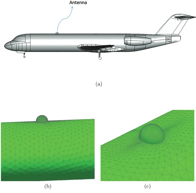
4.2 Antenna mounted on a aircraft, example of structure has small

de-tails on it: (a) aircraft an antenna, (b) mesh, view-1, and (c) mesh, view-2. . . 40

4.3 Huygens’ principle: (a) original problem and (b) tangential

com-ponents of the ﬁelds on the surface. . . 41

4.4 Description of EPA: (a) original problem and (b) decomposed into

(11)

4.5 One-object scattering problem: (a) original problem, (b) outside-inside propagation, (c) solving for current, and (d) outside-inside-outside propagation. . . 44

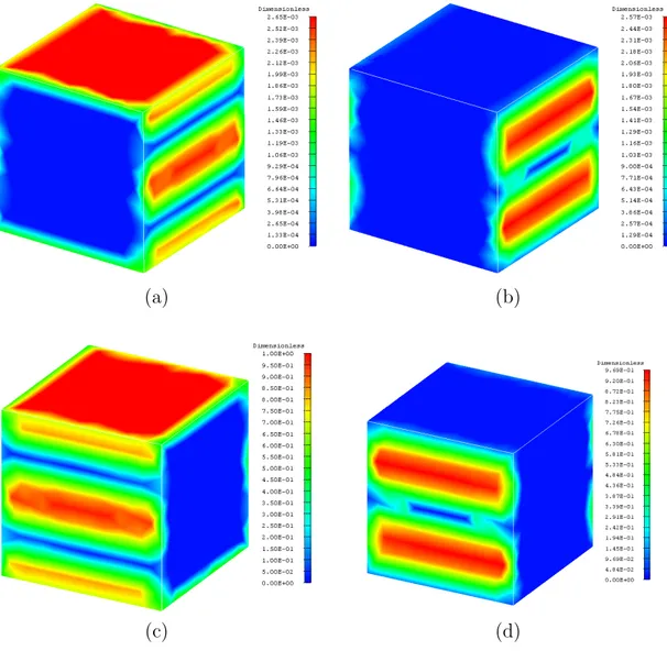
4.6 Example of incident current on a cube with edge length 1λ: (a) real

part of the electric current, (b) imaginary part of the electric cur-rent, (c) real part of the magnetic curcur-rent, and (d) imaginary part

of the magnetic current. . . 46

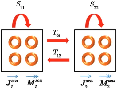
4.7 Example of the interactions among two ESs. . . 52

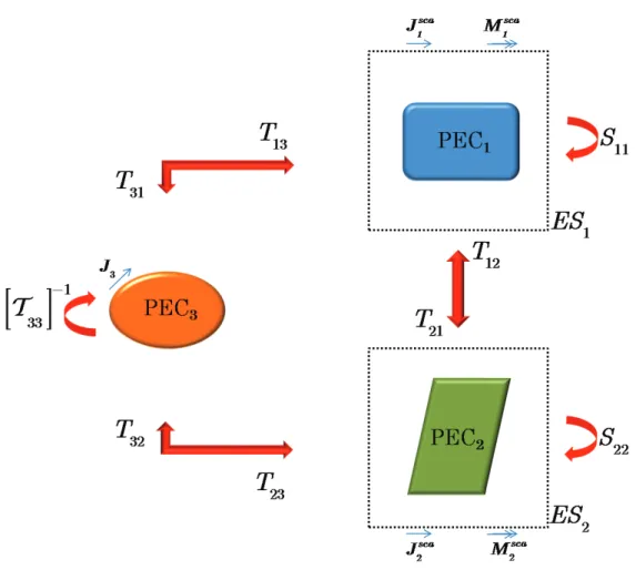
4.8 Example of the interactions among two ESs and one PEC. . . 55

4.9 RCS of PEC sphere: (a) x-y cut, (b) x-z cut, and (c) y-z cut. . . 57

4.10 RCS of PEC cube: (a) x-y cut, (b) x-z cut, and (c) y-z cut. . . . 58

4.11 RCS of two PEC cubes: (a) x-y cut, (b) x-z cut, and (c) y-z cut. 59

4.12 Accuracy test for diﬀerent size of ESs: (a) RCS (x-y cut) of PEC

cube, (b) RCS of PEC cube, and (c) relative error. . . 61

4.13 Accuracy test for diﬀerent size of ESs: (a) RCS of (z-x cut) PEC

4.14 Accuracy test for diﬀerent size of ESs: (a) RSC of (z-y cut) PEC

4.15 Accuracy test for diﬀerent mesh size: (a) RCS (x-y cut) of PEC

4.16 Accuracy test for diﬀerent mesh size: (a) RCS of (z-x cut) PEC

(12)

4.17 Accuracy test for diﬀerent mesh size: (a) RSC of (z-y cut) PEC

4.18 RCS results, distances between ESs is 0.5λ: (a) x-y cut, (b) rel-ative error of x-y cut, (c) z-x cut, (d) relrel-ative error of z-x cut,

(e) z-y cut, and (f) relative error of z-y cut. . . . 67

5.1 Example of the interactions among two ESs. . . 72

5.2 Forward scattered RCS for two PEC cubes as a function of

sub-sections per the sides of ESs. . . 73

5.3 RCS results, when ES is 0.2λ: (a) x-y cut, (b) relative error of

x-y cut, (c) z-x cut, (d) relative error of z-x cut, (e) z-y cut, and

(f) relative error of z-y cut. . . . 75

(f) relative error of z-y cut. . . . 76

(13)

5.6 Accuracy test for diﬀerent mesh size: (a) RCS (x-y cut) of PEC

5.7 Accuracy test for diﬀerent mesh size: (a) RCS (z-x cut) of PEC

5.8 Accuracy test for diﬀerent mesh size: (a) RCS (z-y cut) of PEC

5.9 RCS results, distances between ESs is 0.5λ: (a) x-y cut, (b)

rel-ative error of x-y cut, (c) z-x cut, (d) relrel-ative error of z-x cut,

5.12 Details of the single SRR problem: (a) problem set-up, (b) SRR,

and (c) equivalent surface. . . 85

5.13 Power transmission of single SRR at x = −1.2 mm: (a) power

transmission and (b) relative error. . . 86

5.14 Power transmission of single SRR problem calculated at z = 0 plane for diﬀerent frequencies: (a) 90 GHz, (b) 95 GHz, (c) 97

GHz, (d) 100 GHz, and (e) 105 GHz. . . 87

(14)

5.16 Power transmission of 2× 2 SRR problem calculated at z = 0 plane for diﬀerent frequencies: (a) 90 GHz, (b) 95 GHz, (c) 100

GHz, and (d) 105 GHz. . . 90

5.17 6× 6 SRR wall problem: (a) SRR wall and (b) equivalent surfaces. 91

5.18 Power transmission of 6× 6 SRR problem calculated at z = 0

plane for diﬀerent frequencies: (a) 90 GHz, (b) 95 GHz, (c) 100

GHz, and (d) 105 GHz. . . 92

5.19 10×10 SRR wall problem: (a) SRR wall and (b) equivalent surfaces. 93

5.20 Power transmission of 10× 10 SRR problem calculated at z = 0

plane for diﬀerent frequencies: (a) 90 GHz, (b) 95 GHz, (c) 100

GHz, and (d) 105 GHz. . . 94

5.21 Eﬃciency of the algorithm: (a) number of iterations versus

(15)

To My Family...

Aileme...

(16)

Chapter 1 Introduction

As a general introduction, this chapter describes the relevance of the work, the connection of the existing work and its potential with respect to future applica-tions. We will provide historical context that describes the underlying techniques. Then, we will outline the organization of the thesis.

1.1 Historical Context

In this section, we provide historical overview of computational electromagnetics (CEM). Nowadays, CEM plays very important role in the analysis of the electro-magnetic (EM) phenomena and design of EM systems. With the aid of modern computer technology and numerical algorithms many practical and real-life prob-lems can be modelled and simulated on computers [1].

Among various computational algorithm, method of moments (MoM) is shown to be one of the most versatile and accurate techniques to solve radiation and scattering problems. Nevertheless, the method has some disadvantages. One of the major disadvantage is its high computational cost for memory and time. Due

(17)

to the limited computer capacity, this algorithm usually limited to rather small scale problems [2].

Recently, many researchers focused on developing of efficient fast solvers that ba-sically reduce the computational cost [1]. One of the most successful techniques in this field is fast multipole algorithm (FMA) and its multilevel version mul-tilevel fast multipole algorithm (MLFMA) [3],[4]. These fast solvers are based on iterative solution of matrix equation. Therefore, convergence of an iterative solution is important for the total efficiency of the algorithm. The disadvantage of these fast solvers is convergence of the iterative solvers.

Mainly, if the object has a complicated shape and requires discretization with elements that are very small compared with the wavelength or if the element size varies a lot, convergence of the iterative solvers will be problematic. Feeding structure of the antenna, small antennas mounted on big problems, and metama-terials can be given as examples for these cases. With ﬁrst two real-life problems, some parts of the mesh are much denser than others, which will deteriorate the conditioning of the matrix system, and hence, cause iterative solvers to converge slowly or not converge at all.

Convergence of the iterative solver can be improved by choosing surface inte-gral equation (SIE) formulation properly. Recently, several SIE formulations leading to well-conditioned matrix equation have been developed [3],[5],[6],[7]. Unfortunately, many of these SIE formulations usually lead to a lower solution accuracy [2].

Another way to improve conditioning of the system matrix is preconditioning [8]-[11]. Although effective preconditioners have been developed in recent years, the efficiency of the preconditioner is still problem. Also, preconditioners are for-mulation dependent. Furthermore, it is very difficult to find robust and efficient preconditioner for each problem [12].

(18)

Among various computational algorithms, the domain decomposition method (DDM) is very attractive in solving problems with high complexity. With the capability of dissociation and isolation of the solution of one region from an-other, DDM can be used to facilitate the parallelization of the solution, the reuse of the solution, and also to improve the conditioning of the matrix solu-tion. DDM has been popular with the finite element method [13],[14] and finite difference method [15]-[18]. However, DDM is not popular with the integral equa-tion method. This discrepancy comes from the difficulty of implementing DDM with integral equations. In this thesis, we will present a three-dimensional (3-D) equivalence principle algorithm (EPA) based on DDM and equivalence principle.

1.2 Outline of the Thesis

In this thesis, equivalence principle algorithm is investigated. In Chapter 2, some background information, Maxwell’s equation, boundary conditions, and Huygens’ principle, will be given.

In order to formulate EPA, we will use surface operators. Surface operators and their discretized form are given in Chapter 3 to understand the formulation of EPA. Then, some surface formulations for perfectly electric conductor (PEC), electric-field integral equation (EFIE), magnetic-field integral equation (MFIE), and combined-field integral equation (CFIE) will be given. Also, to discretize the formulations, all necessary tools, MoM and Rao-Wilton-Glisson (RWG) functions will be introduced.

In Chapter 4, we will start with general ideas of EPA. Then using EPA, we will formulate one-object and multi-object scattering problems. At the end of Chapter 4, numerical results will be presented.

(19)

In Chapter 5, tangential-EPA (T-EPA) will be introduced and its accuracy will be compared with EPA.

Finally, in Chapter 6, the main conclusions are drawn of the work that is reported in this thesis and recommendations are given for further development of the EPA method.

(20)

Chapter 2 Background

In the EPA approach, equivalence principle is used to formulate scattering prob-lems in terms of equivalent source distributions. In this chapter, we present the basic theory by which those integral representation may be formulated. Maxwell’s equations, boundary conditions, Huygens’ principle and equivalence principle will be discussed.

2.1 Maxwell’s Equations

The EM ﬁeld is governed by Maxwell’s equations. Together with the constitu-tive relations these equations describe the coupled behavior of the electric and magnetic ﬁeld strengths in space and time.

Faraday’s law of induction:

∇ × E(r, t) = −∂B(r, t)

∂t − M(r, t) (2.1)

Ampere’s circuital law with Maxwell’s extension:

∇ × H(r, t) = ∂D(r, t)

(21)

Gauss’s law:

∇ · D(r, t) = ρe(r, t) (2.3)

Gauss’s Law for magnetism:

∇ · B(r, t) = ρm(r, t) (2.4)

Continuity equation:

∇ · J(r, t) = −∂ρe(r, t)

∂t (2.5)

In the Maxwell’s equations, divergence equations are derivable from curl equa-tions for time varying ﬁelds and current. Hence, there are actually only two equations with four unknown quantities E, H, D, and B, assuming that the driving sources of the system, J and M , are known. The constitutive rela-tions, which describe the material media, have to be invoked to render the above equations solvable.

Constitutive relations:

D(r, t) = ¯ϵ(r)· E(r, t) (2.6)

B(r, t) = ¯µ(r)· H(r, t) (2.7)

Constitutive relations for isotropic medium:

D(r, t) = ϵ(r)E(r, t) (2.8)

B(r, t) = µ(r)H(r, t) (2.9)

Constitutive relations for isotropic and homogeneous medium:

D(r, t) = ϵE(r, t) (2.10)

B(r, t) = µH(r, t) (2.11)

(22)

Linearity of Maxwell’s equations allow us to use Fourier transform and simplify EM equations. F (r, t) = 1 2π ∫ _∞ −∞ dωF (r, ω)e−iωt (2.12)

Substituting (2.12) into the EM equations for the ﬁelds and currents, the equa-tions become independent of time in the Fourier space, but the ﬁelds and currents are now functions of frequency and they are complex valued.

∇ × E(r, ω) = iωµH(r, ω) − M(r, ω) (2.13) ∇ × H(r, ω) = −iωϵE(r, ω) + J(r, ω) (2.14) ∇ · E(r, ω) = 1 ϵρe(r, ω) (2.15) ∇ · H(r, ω) = 1 µρm(r, ω) (2.16)

Similarly, the continuity equation for simple medium in phasor notation can be written as

∇ · J(r, ω) = iωρe(r, ω) (2.17)

2.2 Boundary Conditions

Now, we consider a piecewise smooth stationary interface ∂D, that separates two electromagnetically penetrable regions (region-1 and region-2), as depicted

in Figure 2.1, where the normal ˆn points into region 1. At this interface, a

primary impressed distribution of surface currents, JS and MS, are taken into

account. Boundary conditions are written as

ˆ n× ( E1(r)− E2(r) ) =−MS(r) (2.18) ˆ n× ( H1(r)− H2(r) ) = JS(r) (2.19) ˆ n· ( D1(r)− D2(r) ) = ρe(r) (2.20) ˆ n· ( B1(r)− B2(r) ) =−ρm(r) (2.21)

(23)

Figure 2.1: Stationary boundary surface ∂D between two adjacent domains.

By simplifying the boundary conditions for a PEC surface, we obtain

ˆ n× E1(r) = 0 (2.22) ˆ n× H1(r) = Js(r) (2.23) ˆ n· E1(r) = 1 ϵρes(r) (2.24) ˆ n· H1(r) = 0 (2.25)

2.3 Surface Equivalence Theorem:

Huygens’

Principle

In the analysis of EM problems, sometimes it is easier to form an equivalent problem that yields the same solution within a region of interest. The surface equivalence theorem allows us to replace actual sources with equivalent sources. These ﬁctitious sources are equivalent within the region, because they produce same ﬁelds as actual sources.

(24)

The surface equivalence theorem was introduced in 1963 by Schelkunoﬀ [19], and it is a more rigorous formulation of Huygens’ principle [20], which states [21] that “each point on a primary wavefront can be considered to be a new source of a secondary spherical wave and that a secondary wavefront can be constructed as the envelope of these secondary spherical waves.”

The surface equivalence theorem is based on the uniqueness theorem, which states [22] that “a field in a lossy region is uniquely specified by the sources within the region plus the tangential components of the electric field over the boundary, or the tangential components of the magnetic field over the boundary, or the former over part of the boundary and the latter over the rest of the boundary.” This theorem is also valid for lossless medium. Thus, if the tangential electric and magnetic fields are completely known over a closed surface, the fields in the source-free region can be determined.

Invoking Huygens’ principle, the ﬁeld inside a boundary ∂D that encloses a domain D, may be considered as being generated by an equivalent source distri-bution on that boundary, thereby separating that domain from its environment in an electromagnetic sense.

The associated equivalence source distribution is not unique. To this end, we introduce two distinct equivalence principles, Love’s equivalence principle (LEP) and Schelkunoﬀ’s equivalence principle (SEP). LEP is based on both electric and magnetic equivalent currents. On the other hand, SEP use either electric or magnetic currents. In this thesis, we prefer to use LEP.

Before we introduce an equivalent state, we should ﬁrst deﬁne the corresponding original state. An actual radiating source, which is represented by current

den-sities J1 and M1 is as depicted in Figure 2.2. These original sources radiate and

create EM ﬁelds E1 and H1 everywhere. We want to form an equivalent problem

(25)

Figure 2.2: Original problem.

same ﬁelds outside the closed surface S. The volume within S is denoted by

V1 and outside of S is denoted by V2. An equivalent problem for Figure 2.2 is

shown in Figure 2.3. In Figure 2.3, we assume that there exist ﬁelds E, H inside

S, and ﬁelds E1, H1 outside of S. For these ﬁelds to exist within and outside

S, they must satisfy the boundary conditions about the tangential electric and

magnetic ﬁeld components. Thus, on the imaginary surface S, there must exist

equivalent sources, such that

−ˆn ×(E1(r)− E(r) ) = Ms(r) (2.26) ˆ n× ( H1(r)− H(r) ) = Js(r) (2.27)

These equivalent currents are said to be equivalent within V2, because they will

produce the original ﬁelds only outside of S. Up to this point, we have

intro-duced general form of equivalence theorem. We can also specialize our equivalent

problem by choosing the ﬁelds insideS, appropriately. Fields within S, which is

(26)

are zero, equivalent currents can be rewritten as −ˆn ×(E1(r) ) = Ms(r) (2.28) ˆ n× ( H1(r) ) = Js(r). (2.29)

From these equations, we see that the equivalent currents do not generate any ﬁelds inside V1, while they generate the correct ﬁelds in region V2.

(27)

Chapter 3 Surface Integral Equations

In this chapter, we introduce the SIEs to solve scattering and radiation prob-lems involving 3-D PEC objects having arbitrarily shaped geometries. The SIE method is a versatile numerical technique for solving Maxwell’s equations. Ap-plication of the boundary conditions leads to reduction from a 3-D domain onto its boundary.

In this chapter, we define surface operators, and then we derive EFIE, MFIE and CFIE formulations. For the numerical solution of the problems involving the continuous fields and current density, MoM is introduced. This method expands the current density in terms of known basis functions, and tests the integral equation as many times as the number of unknown coefficients. The result of this method is a linear system to be solved by a suitable technique. Finally, we also provide information about geometry modelling and meshing, triangular basis functions, and discretization of the surface operators.

(28)

3.1 Surface Operators

For surface formulations of scattering and radiation problems, three diﬀerent operators are deﬁned as

T {X}(r) = ik ∫ S dr′ [ X(r′) + 1 k2∇ ′_{· X(r}′₎_∇]_{g(r, r}′₎ _(3.1) K{X}(r) = ∫ S dr′X(r′)× ∇′g(r, r′) (3.2) I{X}(r) = X(r), (3.3)

where S is the closed surface of a 3-D object with an arbitrary shape. In (3.1)–

(3.3), X is either the equivalent electric current (J ), or the equivalent magnetic

current (M ) on the surface, k = ω√µϵ = 2π/λ is the wavenumber, and g(r, r′)

denotes the homogeneous-space Green’s function deﬁned in phasor notation with

the e−iωt convention as

g(r, r′) = exp (ikR) 4πR ( R =|r − r′| ) , (3.4)

where r is observation point, r′ is source point. The operator K is commonly

separated into principal and limit values [23] as

K{X}(r) = KPV{X}(r) − Ωi

4πI

×n_{X}(r), _(3.5)

where 0≤ Ωi ≤ 4π is the internal solid angle, which is nonzero when the

obser-vation point r is on the surface. In (3.5), I×n{X}(r) = ˆn × X(r), where ˆn is

the outward normal unit vector.

Using equivalent surface currents, i.e.,

J (r) = I×n{H}(r) = ˆn × H(r) (3.6)

(29)

secondary (scattered or radiated) electric and magnetic ﬁelds outside the object can be calculated [24] as Esec(r) = ηT {J}(r) − KP V{M}(r) + Ωi 4πI ×n_{M}(r) _(3.8) Hsec(r) = 1 ηT {M}(r) + KP V{J}(r) − Ωi 4πI ×n_{J}(r), _(3.9)

where η =√µ/ϵ is the wave impedance.

3.2 Electric-Field Integral Equation

Scattering from a PEC object is depicted in Figure 3.1. We assume that J

is a current that generates an incident ﬁeld, Einc_{, that impinges on a PEC}

object. Then, electric current will be induced on the PEC object, which in turn radiates to generate the scattered ﬁeld. Applying boundary condition about the

Figure 3.1: Scattering by a PEC object.

tangential component of the electric ﬁeld onS we can derive EFIE as

ˆ

t· Einc(r) + ˆt· Esca(r) = 0, (3.10)

where the observation point r, is located on the surfaceS. As we mentioned

pre-viously, external source or sources generate an incident ﬁeld, Einc_{. The scattered}

electric-ﬁeld, which is represented by Esca can be written as

Esca(r) = iωµ ∫

S′

(30)

where ¯ G(r, r′) = [ I −∇∇ k2 ] g(r, r′). (3.12) ¯

G(r, r′) is the dyadic Green’s function and g(r, r′) is free-space Green’s function

as given in (3.4). By substituting (3.11) into (3.10), EFIE is formed as

ˆ t· ∫ S′ dr′G(r, r¯ ′)· J(r′) = i kηˆt· E inc_(r). _(3.13)

With the aid of surface operators, EFIE can be rewritten as

ˆ

t· ηT {J(r′)} = −ˆt· Einc(r). (3.14)

3.3 Magnetic-Field Integral Equation

In order to derive MFIE, we follow a similar procedure with EFIE. This time we apply the boundary condition about the tangential component of the magnetic ﬁeld on closed surfaces of objects as

ˆ

n× Hinc(r) + ˆn× Hsca(r) = J (r), (3.15)

where the observation point r, approaches the surface S from outside. Similar

to EFIE, external source or sources generates incident ﬁeld Hinc, and Hsca

represents the scattered ﬁeld. The scattered ﬁeld can be written as

Hsca(r) = ∫

S′

dr′J (r′)× ∇′g(r, r′). (3.16)

Then, (3.15) can be rewritten as

J (r)− ˆn ×

∫

S′

dr′J (r′)× ∇′g(r, r′) = ˆn× Hinc(r), (3.17)

which is the general expression for the MFIE. Finally, using K operator and I

operator

(31)

3.4 Combined-Field Integral Equation

Both EFIE and MFIE can be used to solve scattering problems of closed objects. However, both formulations have internal resonance problems at resonance fre-quencies. Internal resonance problem can be avoided by using CFIE [25]. CFIE formulation is basically a linear combination of EFIE and MFIE [25], and can be written as

CFIE = αEFIE + (1− α)MFIE, (3.19)

where α may take values between 0 and 1. Combining (3.13) and (3.17) CFIE can be written as α [ ˆ t· ∫ S′ dr′G(r, r¯ ′)· J(r′) ] + i k(1− α) [ J (r)− ˆn × ∫ S′ dr′J (r′)× ∇′g(r, r′) ] = i k [ α ηˆt· E inc_{(r) + (1}_{− α)ˆn × H}inc_(r) ] , (3.20)

where MFIE part is multiplied by the factor of i/k, in order to balance the equation before linear combination [29].

3.5 Method of Moments

Integral equations introduced in the previous sections can be represented in gen-eral as

L{f(x)} = g(x), (3.21)

whereL is a linear operator, g(x) is known, and f(x) is to be determined. Also,

f (x) and g(x) stands for the current distribution and excitation, respectively. Let f (x) be expanded in a series of functions b1, b2, b3, . . . in the domain ofL,

as f = N ∑ n=1 anbn, (3.22)

(32)

where the an are constants. We shall call the bn expansion functions or basis

functions [26]. We use basis functions to expand the current distribution, so they should be linearly independent and they have to be chosen appropriately.

Substituting (3.22) in (3.21), and using the linearity of L, we have

N

∑

n=1

anL(bn) = g(x). (3.23)

We can deﬁne the residual error as

R(x) =L {∑N n=1 anbn(x) } − g(x) = [∑N n=1 anL{bn(x)} ] − g(x). (3.24)

Then, our aim is to minimize the error in order to solve the problem approxi-mately. Now, we need to deﬁne a set of weighting functions, or testing functions, t1, t2, t3, . . . in the range of L, and take the inner product of (3.23) with each tm. The result is N ∑ n=1 an ⟨ tm(r),L(fn) ⟩ = ⟨ tm(r), g(x) ⟩ (3.25) m = 1,2,3,. . . . This set of equations can be written in matrix form as

¯ Z· a = g. (3.26) ¯ Z =       ⟨ t1(r),L(f1) ⟩ ⟨ t1(r),L(f2) ⟩ . . . ⟨ t2(r),L(f1) ⟩ ⟨ t2(r),L(f2) ⟩ . . . . . . . . . . . .       (3.27) a =      a1 a2 .. .      g =       ⟨ t1(r), g ⟩ ⟨ t2(r), g ⟩ .. .      . (3.28)

We can also deﬁne an inner product as ⟨ a(x), b(x) ⟩ = ∫ dxa(x)· b(x). (3.29)

(33)

So, (3.23) can be tested for m = 1, . . . , N as ∫ dxtm(x)· N ∑ n=1 anL{bn(x)} = ∫ dxtm(x)· g(x). (3.30)

In this step, we can interchange the order of summation and integration. Then, the ﬁnal equation becomes

N ∑ n=1 an ∫ dxtm(x)· L{bn(x)} = ∫ dxtm(x)· g(x), (3.31)

and a linear system can be formed as

N

∑

n=1

anZmn = vm, (3.32)

where the matrix elements are deﬁned as

Zmn =

∫

dxtm(x)· L{bn(x)}, (3.33)

and the vector elements are

vm =

∫

dxtm(x)· g(x). (3.34)

¯

Z is usually called the impedance matrix, and the vector vm is called the

excita-tion vector. An element of the ¯Z matrix at (m, n) is referred to as the interaction

between the mth testing and nth basis functions. The method described above is

called MoM [27]. If the matrix ¯Z is nonsingular, its inverse exists. The

coeﬃ-cients, a, are then given in

a = ¯Z−1v, (3.35)

and the solution for f is given by (3.22). This solution may be exact or

ap-proximate, depending upon the choice of the bn and tm. The particular choice

bn = tm is known as the Galerkin’s method.

3.6 Geometry Modelling and Meshing

Geometries to be solved need to be modelled in the computer environment. After modelling geometries, surfaces of models have to be meshed according to the

(34)

type of basis functions to be used. Figure 3.2 shows triangular meshes applied on sphere and cube models. We use triangular elements for meshing, but it is hard to model the geometry with high accuracy. To reduce the error, we have to decrease the size of elements. However, using small-sized elements lead to large number of triangles or number of unknown coefficients, N [28]. However, it becomes difficult to solve the linear system in (3.26) when N gets larger. So, to solve problem by using MoM both efficiently and accurately, the average size of the elements should be about 1/10 of the wavelength [29].

(a) (b)

Figure 3.2: Discretization by using triangular elements: (a) cube and (b) sphere.

3.7 Triangular Basis Functions

In this thesis, we work with RWG [30] functions, which are linearly varying vector functions deﬁned on planar triangular domains. They have been used as basis and testing functions in MoM applications, because they have some useful properties. RWG functions are deﬁned on two triangles having a common edge

(35)

of length ln. bn(r) =                ln 2A+ n (r− r+_n), r ∈ S_n+ ln 2A−_n(r − n − r), r ∈ Sn− 0, otherwise, (3.36) where A+

n and A−n are areas of the ﬁrst (Sn+) and the second (Sn−) triangles

associated with the edge, respectively. Spatial distribution of RWG functions

are shown in Figure 3.3. So, (3.36) can be rewritten for the function on the nth

Figure 3.3: Spatial distribution of RWG functions.

triangles as

bnb(r) = ± lnb

2An

(r− rnb)δn(r), (3.37)

where δn(r) is used to indicate that the value is one if r is inside the triangle,

and zero otherwise. The alignment of the function on the triangle is represented by the index b = 1, 2, 3. One of the important properties of the RWG functions

(36)

is that their divergence is ﬁnite everywhere. This comes from the fact that there is no discontinuity in the current ﬂow that is crossing the boundaries of the triangles. In general, divergence of the RWG function can be written as

∇ · bn(r) =                ln A+ n , r ∈ S_n+ ln A−_n, r ∈ S − n 0, otherwise. (3.38)

The total charge associated with the function becomes

A+_n ln A+ n − A− n ln A−_n = 0. (3.39)

Implementing EFIE with MoM requires divergence operation on the current den-sity and also requires the divergence of the testing functions. Therefore, it is suitable to use RWG functions as both the basis and the testing functions.

3.8 Discretization of Surface Operators

For numerical solutions of equivalent electric (Jinc) and magnetic (Minc) currents on the equivalent surface, we discretize surfaces by using small planar triangles and employ basis functions to expand unknown surface current densities, i.e.,

Jinc(r) =−ˆn × Hinc(r)≈ N ∑ n=1 aJ_nbn(r) (3.40) Minc(r) = ˆn× Einc(r)≈ N ∑ n=1 aM_n bn(r), (3.41)

where bn represents the nth basis function associated with the nth edge.

Test-ing integral equations on the surface, N× N matrix equations are constructed.

Elements of the system matrix correspond to interactions of basis and testing functions, while excitation vector is obtained by testing the incident ﬁelds. Ma-trix elements involve discretized surface operators depending on the

formula-tion. Considering the nth _{basis function b}

(37)

tangentially-tested and normally-testedK, T , and I operators are discretized as ˆ t· KP V = ∫ Sm drtm(r)· KP V{bn}(r) (3.42) ˆ n× KP V = ∫ Sm drtm(r)· ˆn × KP V{bn}(r) (3.43) ˆ t· T = ∫ Sm drtm(r)· T {bn}(r) (3.44) ˆ n× T = ∫ Sm drtm(r)· ˆn × T {bn}(r) (3.45) ˆ t· I = ∫ Sm drtm(r)· I{bn}(r) (3.46) I×n₌∫ Sm drtm(r)· I{bn}(r) × ˆn. (3.47)

Elements of excitation vectors in (3.34) also depend on the formulation. They involve tangential and normal testing of incident electric and magnetic ﬁelds, i.e.,

v_mE,T = ∫ Sm drtm(r)· Einc(r) (3.48) vE,N_m = ∫ Sm drtm(r)· ˆn × Einc(r) (3.49) v_mH,T = ∫ Sm drtm(r)· Hinc(r) (3.50) v_mH,N = ∫ Sm drtm(r)· ˆn × Hinc(r). (3.51)

Interaction between the mth _{testing function t}

m, and the nth basis function bn

need to be derived for diﬀerent operators (T , K, and I) and for diﬀerent testing

types (tangential and normal). We discretize all operators by employing RWG functions. Then, interactions modiﬁed and divided into smaller basic integrals.

Let’s start with tangentially-testedT operator.

¯ TT[m, n] = ik ∫ Sm drtm(r)· ∫ Sn dr′g(r, r′)bn(r′) + i k ∫ Sm drtm(r)· ∫ Sn dr′∇g(r, r′)∇′· bn(r′) (3.52) Using divergence-conforming functions, such as the RWG functions, and using identity (3.53), the interaction in (3.52) is modiﬁed as

(38)

¯ TT[m, n] = ik ∫ Sm drtm(r)· ∫ Sn dr′g(r, r′)bn(r′) + i k ∫ Sm drtm(r)· ∇ ∫ Sn dr′g(r, r′)∇′· bn(r′) = ik ∫ Sm drtm(r)· ∫ Sn dr′g(r, r′)bn(r′) + i k ∫ Sm dr∇ · { tm(r) ∫ Sn dr′g(r, r′)∇′· bn(r′) } − i k ∫ Sm dr∇ · tm(r) ∫ Sn dr′g(r, r′)∇′· bn(r′) = ik ∫ Sm drtm(r)· ∫ Sn dr′g(r, r′)bn(r′) − i k ∫ Sm dr∇ · tm(r) ∫ Sn dr′g(r, r′)∇′· bn(r′). (3.54) In the second term, we move diﬀerential operator onto the testing function [30],

hence, the hyper-singularity of theT operator is eliminated. Then,

tangentially-tested T operator expression can be rewritten as,

¯ TT[m, n] = ik [ ∫ Sm drtm(r)· ∫ Sn dr′g(r, r′)bn(r′) − 1 k2 ∫ Sm dr∇ · tm(r) ∫ Sn dr′g(r, r′)∇′ · bn(r′) ] . (3.55)

Inserting the RWG functions and their divergences explicitly by using (3.36) and (3.38), ¯ TT[m, n, a, b] = ik [ lma 2Am γma lnb 2An γnb ∫ Sm dr(r− rma)· ∫ Sn dr′g(r, r′)(r′− rnb) − 1 k2 lma Am lnb An γmaγnb ∫ Sm dr ∫ Sn dr′g(r, r′) ] , (3.56)

then, by factoring out common terms,

¯ TT[m, n, a, b] = ikCma,nb [ ∫ Sm dr(r− rma)· ∫ Sn dr′g(r, r′)(r′− rnb) − 4 k2 ∫ Sm dr ∫ Sn dr′g(r, r′) ] , (3.57)

where n and m indicate the interaction is between nth _{and m}th _{triangles, while a}

and b represent the alignment of the basis and testing functions on these triangles.

The coeﬃcient Cma,nb can be written as

Cma,nb=

γmalmaγnblnb

4AmAn

(39)

In the evaluation of these integrals, it obvious that the integrands tend to diverge as the observation point approaches the source point, due to the singularity of the Green’s function. By using singularity extraction method [31], problematic inner integral can be divided into analytical and numerical parts, each of which can be evaluated without any problem [30],[32],[33]. In order to easily evaluate the analytical integrals appearing in the singularity extraction, we apply a coordinate transformation, so that the basis triangle lies on the x-y plane with one of its edges lying on the x-axis [29]. The ﬁrst part of (3.57) can be written as,

∫ Sm dr(r− rma)· ∫ Sn dr′g(r, r′)(r′− rnb) = ∫ Sm dr(x− xma) ∫ Sn dr′g(r, r′)(x′ − xnb) + ∫ Sm dr(y− yma) ∫ Sn dr′g(r, r′)(y′ − ynb) + ∫ Sm dr(z− zma) ∫ Sn dr′g(r, r′)(z′− znb). (3.59) After applying rotation such that,

z′ → 0, znb → 0 (3.60) (3.59) becomes, ∫ Sm dr(r− rma)· ∫ Sn dr′g(r, r′)(r′− rnb) = ∫ Sm dr(x− xma) ∫ Sn dr′g(r, r′)(x′ − xnb) + ∫ Sm dr(y− yma) ∫ Sn dr′g(r, r′)(y′ − ynb). (3.61) two scalar equations in (3.61) can be rewritten as follow:

∫ Sm dr(x− xma) ∫ Sn dr′g(r, r′)(x′− xnb) = ∫ Sm drx ∫ Sn dr′g(r, r′)x′ − xnb ∫ Sm drx ∫ Sn dr′g(r, r′) − xma ∫ Sm dr ∫ Sn dr′g(r, r′)x′ + xnbxma ∫ Sm dr ∫ Sn dr′g(r, r′), (3.62)

(40)

∫ Sm dr(y− yma) ∫ Sn dr′g(r, r′)(y′ − ynb) = ∫ Sm dry ∫ Sn dr′g(r, r′)y′ − ynb ∫ Sm dry ∫ Sn dr′g(r, r′) − yma ∫ Sm dr ∫ Sn dr′g(r, r′)y′ + ymaynb ∫ Sm dr ∫ Sn dr′g(r, r′). (3.63) Now, we can deﬁne three inner integrals as

Iin1 = ∫ Sn dr′g(r, r′), (3.64) Iin2 = ∫ Sn dr′x′g(r, r′), (3.65) Iin3 = ∫ Sn dr′y′g(r, r′). (3.66)

Finally, the tangentially-tested T operator involves seven basic integrals, i.e.,

¯ TT[m, n, a, b] = ikCma,nb [ (xmaxnb+ ymaynb− 4 k2)I1+ I2+ I3− xnbI4

− xmaI5− ynbI6− ymaI7 ] , (3.67) where I1 = ∫ Sm dr′Iin1, I5 = ∫ Sm dr′Iin2, I2 = ∫ Sm dr′xIin2, I6 = ∫ Sm dr′yIin1, I3 = ∫ Sm dr′yIin3, I7 = ∫ Sm dr′Iin3. I4 = ∫ Sm dr′xIin1, (3.68)

After testing T operator tangentially, we divide whole interaction into basic

integrals, so that we can apply similar procedures, for K operator. Substituting

(3.36) and (3.38), into (3.42), ¯ KT[m, n, a, b] = γmaγnb 4AmAn ∫ Sm dr(r− rma)· ∫ Sn dr′(r′ − rnb)× ∇′g(r, r′). (3.69) Then, the gradient of the Green’s function can be written explicitly as,

∇′_{g(r, r}′_{) =} eikR(1− ikR)

4πR3 (r− r

(41)

Using (3.70) and (3.69) becomes, ¯ KT[m, n, a, b] = γmaγnb 4AmAn ∫ Sm dr(r− rma)· ∫ Sn dr′(r′− rnb) ×eikR(1− ikR) 4πR3 (r− r ′_), _(3.71) ¯ KT[m, n, a, b] = γmaγnb 16πAmAn ∫ Sm dr(r− rma)· ∫ Sn dr′(r′− rnb) ×(r − r′₎eikR(1− ikR) R3 . (3.72)

By using identity showed in (3.73), we obtain the ﬁnal form of (3.69) as

(r′− rnb)× (r − r′) = −(r − rnb)× (r′ − r), (3.73) ¯ KT[m, n, a, b] =− γmaγnb 16πAmAn ∫ Sm dr(r− rma)· (r − rnb) × ∫ Sn dr′(r′− r)e ikR₍₁_{− ikR)} R3 . (3.74)

Next, (3.74) is decomposed into three scalar equations as follows: ∫ Sn dr′(r′− r)e ikR₍₁_{− ikR)} R3 = ˆx ∫ Sn dr′(x′ − x)e ikR₍₁_{− ikR)} R3 + ˆy ∫ Sn dr′(y′− y)e ikR₍₁_{− ikR)} R3 + ˆz ∫ Sn dr′(z′− z)e ikR₍₁− ikR) R3 . (3.75)

Similarly, for K operator, applying rotation such that,

z′ → 0 (3.76) (3.75) becomes; ∫ Sn dr′(r′− r)e ikR₍₁_{− ikR)} R3 = ˆx ∫ Sn dr′(x′− x)e ikR₍₁_{− ikR)} R3 + ˆy ∫ Sn dr′(y′ − y)e ikR₍₁− ikR) R3 − ˆz ∫ Sn dr′ze ikR₍₁_{− ikR)} R3 . (3.77)

(42)

Deﬁning three inner integrals as Iin1 = ∫ Sn dr′(x′− x)e ikR₍₁_{− ikR)} R3 , (3.78) Iin2 = ∫ Sn dr′(y′− y)e ikR₍₁_{− ikR)} R3 , (3.79) Iin3 = ∫ Sn dr′ze ikR₍₁_{− ikR)} R3 , (3.80)

and taking curl operation with some modiﬁcations we obtain

(r− rnb)× (ˆxIin1+ ˆyIin2+ ˆzIin3) = ˆx

[

− (y − ynb)Iin3− zIin2)

] + ˆy [ (x− xnb)Iin3+ zIin1) ] + ˆz [

(x− xnb)Iin2− (y − ynb)Iin1)

] , (3.81) ¯ KT[m, n, a, b] =− γmaγnb 16πAmAn ∫ Sm dr(x− xma) [

− (y − ynb)Iin3− zIin2)

] + (y− yma) [ (x− xnb)Iin3+ zIin1) ] + (z− zma) [

(x− xnb)Iin2− (y − ynb)Iin1)

]

. (3.82)

Finally, we end-up with the following equation

¯ KT[m, n, a, b] =− γmaγnb 16πAmAn ∫ Sm dr [

− xyIin3+ xynbIin3− xzIin2 + yxmaIin3 − ynbxmaIin3+ zxmaIin3+ yzIin1+ xyIin3− yxnbIin3 − zymaIin1 − xymaIin1+ ymaxnbIin3+ zxIin2− zxnbIin2− xzmaIin2+ zmaxnbIin2 − yzIin1+ zxnbIin1

]

. (3.83)

As a result, tangentially-tested K operator involves nine basic integrals, i.e.,

¯ KT[m, n, a, b] =− γmaγnb 16πAmAn [ (ynb− yma)I1+ zmaI2 − zmaynbI3+ (xma− xnb)I4 − zmaI5+ zmaxnbI6+ (ynb− yma)I7+ (xma− xnb)I8 + (ymaxnb− xmaynb)I9

]

(43)

where I1 = ∫ Sm dr′zIin1, I4 = ∫ Sm dr′zIin2, I7 = ∫ Sm dr′xIin3, I2 = ∫ Sm dr′yIin1, I5 = ∫ Sm dr′xIin2, I8 = ∫ Sm dr′yIin3, I3 = ∫ Sm dr′Iin1, I6 = ∫ Sm dr′Iin2, I9 = ∫ Sm dr′Iin3. (3.85)

The next operator is normally-testedT operator, which can be written as,

ˆ n× T = ∫ Sm drtm(r)· ˆn × T {bn}(r). (3.86) Substituting (3.1) into (3.86) ¯ TN[m, n] = ik ∫ Sm drtm(r)· ˆn × ∫ Sn dr′g(r, r′)bn(r′) + i k ∫ Sm drtm(r)· ˆn × ∫ Sn dr′∇g(r, r′)∇′ · bn(r′). (3.87) Then, using (3.36) and (3.38) we obtain

¯ TN[m, n, a, b] = ik lma 2Am γma lnb 2An γnb ∫ Sm dr(r− rma)· ˆn × ∫ Sn dr′g(r, r′)(r′− rnb) + i k ∫ Sm dr lma 2Am γma(r− rma)· ˆn × ∫ Sn dr′∇g(r, r′)lnb Anγnb, (3.88) where Cma,nb= γmalmaγnblnb 4AmAn . (3.89) Finally, we obtain, ¯ TN[m, n, a, b] = ikCma,nb [ ∫ Sm dr(r− rma)· ˆn × ∫ Sn dr′g(r, r′)(r′ − rnb) + 2 k2 ∫ Sm dr(r− rma)· ˆn × ∫ Sn dr′∇g(r, r′) ] . (3.90)

Furthermore, gradient of Green’s function with respect to unprimed coordinates can be calculated as

∇g(r, r′_{) =} eikR(1− ikR)

4πR3 (r

(44)

Then, we obtain ¯ TN[m, n, a, b] = ikCma,nb [ ∫ Sm dr(r− rma)· ∫ Sn dr′g(r, r′)ˆn× (r′ − rnb) + 2 k2 ∫ Sm dr(r− rma)· ˆn × ∫ Sn dr′e ikR₍₁_{− ikR)} 4πR3 (r ′_{− r)} ] . (3.92) As we have done previously, we decompose (3.92) into three scalar equations,

∫ Sn dr′(r′− r)e ikR₍₁_{− ikR)} R3 = ˆx ∫ Sn dr′(x′ − x)e ikR₍₁_{− ikR)} R3 + ˆy ∫ Sn dr′(y′− y)e ikR₍₁− ikR) R3 + ˆz ∫ Sn dr′(z′− z)e ikR₍₁_{− ikR)} R3 . (3.93) By applying rotation as z′ → 0 (3.94) we obtain ∫ Sn dr′(r′− r)e ikR₍₁− ikR) R3 = ˆx ∫ Sm dr′(x′− x)e ikR₍₁− ikR) R3 + ˆy ∫ Sn dr′(y′− y)e ikR₍₁_{− ikR)} R3 − ˆz ∫ Sn dr′ze ikR₍₁_{− ikR)} R3 . (3.95)

If we deﬁne inner integrals as

Iin1 = ∫ Sn dr′(x′ − x)e ikR₍₁_{− ikR)} R3 (3.96) Iin2 = ∫ Sn dr′(y′− y)e ikR₍₁− ikR) R3 (3.97) Iin3 = ∫ Sn dr′e ikR₍₁− ikR) R3 , (3.98) ¯ TN[m, n, a, b] = ikCma,nb [ ∫ Sm dr(r− rma)· ∫ Sn dr′g(r, r′)ˆn× (r′ − rnb) + 2 k2 ∫ Sm

dr(r− rma)· ˆn × (Iin1+ Iin2+ Iin3)

]

(45)

and if we calculate the curl of second part and apply dot product, 2

k2 ∫

Sm

dr(r− rma)· ˆn × (Iin1+ Iin2 + Iin3)

= 2 k2 ∫ Sm dr [

xnyIin3− xnzIin2 − xnbnyIin3+ xnbnzIin2+ ynzIin1 − ynxIin3 − ynbnzIin1+ ynbnxIin3+ znxIin2− znyIin1− znbnxIin2+ znbnyIin1

]

.

(3.100) We apply similar procedure to the ﬁrst part of the equation. Due to rotation,

z′ → 0, znb → 0 (3.101) Iin4 = ∫ Sn dr′e ikR 4πR (3.102) Iin5 = ∫ Sn dr′x′e ikR 4πR (3.103) Iin6 = ∫ Sn dr′y′e ikR 4πR. (3.104) Then, we obtain ∫ Sm dr(r− rma)· ∫ Sn dr′g(r, r′)ˆn× (r′− rnb) = ∫ Sm dr [

− nzxIin6 + ymanzxIin4+ xnbnzIin6− xnbymanzIin4 + nzyIin5 − xmanzyIin4− ynbnzIin5+ ynbxmanzIin4+ znxIin6− zymanxIin4− zIin5ny

+ zxmanyIin4− znbIin6nx+ znbymanxIin4+ znbIin5ny − znbxmanyIin4

]

.

(3.105)

By combining the ﬁrst and second parts of the equation, the normally-tested T

operator involves 19 basic integrals, i.e.,

¯ TN[m, n, a, b] = ikCma,nb ([ (ymaxnbnz− xmaynbnz+ zmaynbnx− zmaxnbny)I10 + (zmany− ymanz)I14+ (xmanz− zmanx)I17+ ynbnzI11+ nzI5 − xnbnzI4− nzI18+ nxI19− nyI16+ (xnbny − ynbnx)I13 ] + 2 k2 [ nyI8 − nzI5+ nzI2 − nxI9+ nxI6 − nyI3+ (zmany − ymanz)I1 + (xmanz− zmanx)I4+ (ymanx− xmany)I7 ]) , (3.106)

(46)

where I1 = ∫ Sm dr′Iin1, I8 = ∫ Sm dr′xIin3, I15= ∫ Sm dr′yIin5, I2 = ∫ Sm dr′yIin1, I9 = ∫ Sm dr′yIin3, I16 = ∫ Sm dr′zIin5, I3 = ∫ Sm dr′zIin1, I10= ∫ Sm dr′Iin4, I17= ∫ Sm dr′Iin6, I4 = ∫ Sm dr′1Iin2, I11 = ∫ Sm dr′xIin4, I18= ∫ Sm dr′xIin6, I5 = ∫ Sm dr′xIin2, I12= ∫ Sm dr′yIin4, I19= ∫ Sm dr′zIin6. I6 = ∫ Sm dr′zIin2, I13= ∫ Sm dr′zIin4, I7 = ∫ Sm dr′Iin3, I14= ∫ Sm dr′Iin5, (3.107)

The next operator is normally-testedK operator deﬁned as

ˆ n× KP V = ∫ Sm drtm(r)· ˆn × KP V{bn}(r) (3.108) ¯ KN[m, n] = ∫ Sm drtm(r)· ˆn × ∫ Sn dr′bn(r′)× ∇′g(r, r′) (3.109) ¯ KN[m, n, a, b] = γmaγnb 4AmAn ∫ Sm dr(r− rma)· ˆn × ∫ Sn dr′(r′ − rnb) ×eikR(1− ikR) 4πR3 (r− r ′_). _(3.110)

By using identity (3.73) and (3.110) can be rewritten as

¯ KN[m, n, a, b] = γmaγnb 16πAmAn ∫ Sm dr(r− rma)· ˆn × (rnb− r) × ∫ Sn dr′(r′− r)e ikR₍₁_{− ikR)} R3 . (3.111)

Further, by using (3.75), (4.30) and result of (3.81), calculating the curl of the

(47)

obtain ¯ KN[m, n, a, b] = γmaγnb 16πAmAn [ (nxzma− xmanz)I4+ (ynbnz+ ymanz − zmany)I19 + nxI13− (ymaynbnx+ xmaynbny)I1+ (ymanx+ ynbnx− xmany)I3 − nxI7+ (xnbny+ xmany− ymanx)I10− (xmaxnbny+ ymaxnbnx)I9

− nyI15− nxI8+ nzI6+ nzI14− nxxnbI11− nyI16− nyynbI2 + (zmaxnbnx+ zmaynbny− xmaxnbnz− ymaynbnz)I17− nzI23 + (nyzma− ymanz)I12+ (xnbnz+ xmanz− zmanx)I18− nzI24 − (nxxnb+ ynbny)I20+ nyI21+ nyI22nyI5 ] , (3.112) where I1 = ∫ Sm dr′Iin1, I9 = ∫ Sm dr′Iin2, I17= ∫ Sm dr′Iin3, I2 = ∫ Sm dr′xIin1, I10= ∫ Sm dr′xIin2, I18 = ∫ Sm dr′xIin3, I3 = ∫ Sm dr′yIin1, I11 = ∫ Sm dr′yIin2, I19= ∫ Sm dr′yIin3, I4 = ∫ Sm dr′zIin1, I12= ∫ Sm dr′zIin2, I20 = ∫ Sm dr′zIin3, I5 = ∫ Sm dr′xyIin1, I13= ∫ Sm dr′xzIin2, I21 = ∫ Sm dr′xzIin3, I6 = ∫ Sm dr′xzIin1, I14 = ∫ Sm dr′yzIin2, I22 = ∫ Sm dr′yzIin3, I7 = ∫ Sm dr′y2Iin1, I15= ∫ Sm dr′x2Iin2, I23= ∫ Sm dr′x2Iin3, I8 = ∫ Sm dr′z2Iin1, I16= ∫ Sm dr′y2Iin2, I24= ∫ Sm dr′y2Iin3. (3.113) The last operator isI operator. In order to discretize this operator, we will start

with tangentially-testedI. By using (3.36)

ˆ t· I = ∫ Sm drtm(r)· I{bn}(r) (3.114) ¯ IT[n, n, a, b] = ∫ Sn drtn(r)· bn(r) = γnγna lnb 2An lna 2An ∫ Sn dr(r− rnb)· (r − rna) (3.115)

(48)

The integrand of the (3.115) can be written explicitly as

(r− rnb)· (r − rna) = x2+ y2+ z2− xxna− yyna− zzna− xxxb

− yynb− zznb+ xnaxnb+ ynaynb+ znaznb. (3.116)

Substituting (3.116) into (3.115) we obtain

¯ IT[n, n, a, b] = γnbγna lnblna 4A2 n ∫ Sn dr [

x2+ y2+ z2− xxna− yyna − zzna

− xxxb− yynb− zznb+ xnaxnb+ ynaynb+ znaznb

]

. (3.117)

Then, we can separate whole integral into basic integrals, such that,

I1 = ∫ Sn dr′x2, I5 = ∫ Sn dr′z2, I2 = ∫ Sn dr′x, I6 = ∫ Sn dr′z, I3 = ∫ Sn dr′y2, I7 = ∫ Sn dr′. I4 = ∫ Sn dr′y, (3.118)

By using basic integrals, (3.114) will result,

¯ IT[n, n, a, b] = γnbγna lnblna 4A2 n [ I1− (xnb+ xna)I2+ I3− (ynb+ yna)I4 + I5− (znb+ zna)I6+ (xnaxnb+ ynaynb+ znaznb)I7 ] . (3.119)

Finally, normally-testedI operator is examined.

¯ IN[n, n] = ∫ Sn drtn(r)· I{bn}(r) × ˆn, (3.120) ¯ IN[n, n, a, b] = γnbγna lnb 2An lna 2An ∫ Sn dr(r− rnb)· (r − rna)× ˆn,

(49)

where

(r− rnb)· (r − rna)× ˆn = [

(xy− xyna− xnby + xnbyna)nz − (zx − zxnb− znax + znaxnb)ny

+ (zy− zynb− znay + znaynb)nx − (xy − xynb− xnay + xnaynb)nz

+ (yz− yznb− ynaz + ynaznb)nx − (xz − xznb− xnaz + xnaznb)ny

]

. (3.121)

Substituting (3.121) into (3.120) we obtain

¯ IN[n, n, a, b] = γnbγna lnblna 4A2 n ∫ Sn dr [ (xnbynanz− znaxnbny+ znaynbnx+ ynaznbnx − xnaznbny− xnaynbnz)I1− 2nyI6+ (nx+ ny)I5+ (xnbny − ynbnx − ynanx+ xnany)I4+ (znbny− ynanz+ znany+ ynbnx)I2+ (xnanz − xnbnz − znanx− znbnx)I3 ] , (3.122) where I1 = ∫ Sn dr′, I4 = ∫ Sn dr′z, I2 = ∫ Sn dr′x, I5 = ∫ Sn dr′yz, I3 = ∫ Sn dr′y, I6 = ∫ Sn dr′zx. (3.123)

After discretizing operators on the left-hand-side (LHS), we discretize the possi-ble right-hand-side (RHS) of the matrix equation as

vE,T[m] = ∫ Sm drtm(r)· Einc(r) (3.124) vE,N[m] = ∫ Sm drtm(r)· ˆn × Einc(r) (3.125) vH,T[m] = ∫ Sm drtm(r)· Hinc(r) (3.126) vH,N[m] = ∫ Sm drtm(r)· ˆn × Hinc(r). (3.127)

Solution of electromagnetics problems with the equivalence principle algorithm

SOLUTION OF ELECTROMAGNETICS

PROBLEMS WITH THE EQUIVALENCE

PRINCIPLE ALGORITHM

a thesis

submitted to the department of electrical and

electronics engineering

and the institute of engineering and science

of bilkent university

in partial fulfillment of the requirements

for the degree of

master of science

By

Burak Tiryaki

September 2010

ABSTRACT

SOLUTION OF ELECTROMAGNETICS

PROBLEMS WITH THE EQUIVALENCE

PRINCIPLE ALGORITHM

Burak Tiryaki

M.S. in Electrical and Electronics Engineering

Supervisor: Prof. Dr. Levent G¨

urel

September 2010

¨

OZET

ELEKTROMANYET˙IK PROBLEMLER˙IN ES

¸DE ˘

GERL˙IK

PRENS˙IB˙I Y ¨

ONTEM˙IYLE C

¸ ¨

OZ ¨

UMLER˙I

Burak Tiryaki

Elektrik ve Elektronik M¨

uhendisli˘

gi B¨

ol¨

um¨

u Y¨

uksek Lisans

Tez Y¨

oneticisi: Prof. Dr. Levent G¨

urel

Eyl¨

ul 2010

ACKNOWLEDGMENTS

Contents

List of Figures

To My Family...

Aileme...

Chapter 1

Introduction

1.1

Historical Context

1.2

Outline of the Thesis

Chapter 2

Background

2.1

Maxwell’s Equations

2.2

Boundary Conditions

2.3

Surface Equivalence Theorem:

Huygens’

Principle

Chapter 3

Surface Integral Equations

3.1

Surface Operators

3.2

Electric-Field Integral Equation

3.3

Magnetic-Field Integral Equation

3.4

Combined-Field Integral Equation

3.5

Method of Moments