A new load balancing heuristic using self-organizing maps

(1)

(2)

A NEW LOAD BALANCING HEURISTIC USING

SELF-ORGANIZING MAPS

A THESIS

SUBMITTED TO THE DEPARTMENT OF COMPUTER

ENGINEERING AND INFORMATION SCIENCE

AND THE INSTITUTE OF ENGINEERING AND SCIENCE

OF BILKENT UNIVERSITY

IN PARTIAL FULFILLMENT OF THE REQUIREMENTS

FOR THE DEGREE OF

MASTER OF SCIENCE

By

Murat Atım

September, 1999

(3)

Z t ^ 6 1 ’ 'ü 5 ^ o £6 \

(4)

I certify that I have read this thesis and that in my opin ion it is fully adequate, in scope and in quality, as a thesis for the degree of Master of Science.

AsshMProh A tt iû ^ upervisor)

iir ÜİUSC

Ai»oc. Prof. Özgür Ülusoy

Cevdet Aykanat

Approved for the Institute of Engineering and Science:

Prof. Mehn^^rjaray

(5)

ABSTRACT

A NEW LOAD BALANCING HEURISTIC USING

SELF-ORGANIZING MAPS

Murat Atun

M. S. in Computer Engineering and Information Science

Supervisor: Asst. Prof. Attila Gürsoy

September, 1999

In order to have an optimal performance during an execution of a parallel program, the tasks of the parallel computation must be mapped to processors such that the computational load is distributed as evenly as possible while highly communicating tasks are placed closely. We describe a new algorithm for static load balancing problem based on Kohonen Self-Organizing Maps (SOM) which preserves the neighborhood relationship of tasks. We define the input space of the SOM algorithm to be a unit square and divide it into “number of processors” regions. The tasks are represented by the neurons which are mapped to the regions randomly. We enforce load balancing by selecting training input from the region of the least loaded processor. We e.xamine the impact of various input selection strategies and neighborhood functions on the accuracy of the mapping. The results show that our algorithm outperforms the other task mapping algorithms implemented with SOMs.

Key words: Neural networks, Self-Organizing Maps, Kohonen, tcisk map ping, load balancing.

(6)

ÖZET

KENDİNDEN DÜZENLENEN HARİTALAR ALGORİTMASI

KULLANAN YENİ BİR SEZGİSEL YÜK DENGELEME

ALGORİTMASI

Murat Atım

Bilgisayar ve Enformatik Mühendisliği Bölümü Yüksek Lisans

Tez Yöneticisi; Yrd. Doç. Attila Gürsoy

Eylül, 1999

Koşut bir programın çalışması sırasında en iyi başarımın elde edilebilmesi için, görevlerin yüklerinin mümkün olduğu kadar eşit dağıtılması aynı zamanda yüksek oranlı iletişimde bulunan görevlerin de göreceli olarak yakın işlemcilere atanmaları gerekmektedir. Bu çalışmada, durgun yük dağıtımı için “Kendin den Düzenlenen Haritalar” algoritmasının yeni bir gerçekleştirimini sunduk. Kohonen’nin bu algoritması bilindiği üzere topolojik özellikleri koruyan bir al goritmadır. Biz girdi uzayını, birim kare olarak tanımladık ve bu uzayı, işlemci sayısı kadar parçaya böldük. Her seferinde Kohonen algoritmasının girdisini en az yüke sahip işlemcinin bölgesinden seçerek, algoritmaya eşit yük dağıtım özelliğini entegre ettik. Girdi seçimi, komşuluk çapı işlevi ve çalışma adım sayısı işlevlerinin varyasyonları incelenerek en iyi sonucu verenler tespit edildi. Sonuçlar, algoritmamızın. Kendinden Düzenlenen Haritalar algoritması kul lanılarak gerçekleştirilmiş diğer algoritmalardan çok daha iyi sonuçlar verdiğini göstermektedir.

Anahtar Kelimeler: Sinir ağları. Kendinden Düzenlenen Haritalar, Koho nen, görev atama, yük dengeleme.

(7)

(8)

Acknowledgement

First of all, I would like to express my deepest gratitude to my advisor Asst. Prof. Attila Gürsoy for his great supervision, guidance and patience for the development of this thesis.

I would like to thank to committee members Özgür Ulusoy and Cevdet Aykanat for reading the thesis and for their constructive comments.

I also would like to thank to my fiancée Yeşim for her great patience and advices, my friends Emek and İlker for their invaluable friendship and finally to my family for their moral support.

(9)

List of Figures

3.1 Typiccil Som A lgorithm ... 11

3.2 Sample Execution of S O M ... ' ... 13

4.1 Input S p a c e ... 15

4.2 Input and Output S p a c e ... 15

4.3 Subregions of processor regions 17 4.4 Gaussian Neighbourhood Function 20 4.5 Execution states for a simple graph at steps 0, 50 and 400 22 4.6 Execution states for a simple graph at steps 3200, 5200 and 20000 22 5.1 Subregion selection by “Gaussian Distribution with Distance In formation” ... 26

5.2 Subregion selection by “Gaussian Distribution with Region In formation” ... 27

6.1 A twisted mapping (a) and Expected mapping ( b ) ... 37

7.1 Sample mapping for ..lagmesh for steps 1000,2000 and 4000 48 7.2 Sample mapping for .Jagmesh for steps 8000,12000 and 16000 . . 48

(12)

7.3 Trend Line Chart for 16 processors 52 7.4 Trend Line Chart for 32 processors 52

7.5 Trend Line Chart for Coefficient a ... 53

7.6 Trend Line Chart for Coefficient b ... 53

8.1 Sample mapping of Whitaker on 16 p rocessors... 61

8.2 Sample mcipping of L on 8 p rocessors... 61

8.3 Sample mapping of StufelO on 8 processors... 62

A-1 Chaco Input File F orm a t... 72

C-1 Whole Execution results for 128 processors (Steps Impact) 76 C-2 Whole Execution results for 64 processors (Steps Impact) . . . . 77

C-3 Whole Execution results for 32 proces,sors (Steps Impact) . . . . 78

C-4 Whole Execution results for 16 processors (Steps Impact) . . . . 79 C-5 Whole Execution results for 8 processors (Steps Impact) 80

(13)

List of Tables

5.1 Load Imbalance results for 16 processors(%) 29 5.2 Load Imbalance results for 32 processors(%) 29 5.3 Load Imbalance results for PRO-DLL (%)(16 processors) . . . . 31 5.4 Communication Cost results for PRO-DLL (xl0000)(16 proces

sors) ... 31 5.5 Load Imbalance results for PRO-DLL (%)(32 processors) . . . . 32

5.6 Communication Cost results for PRO-DLL (xl0000)(32 proces

sors) 32

5.7 Grouped Load Imbalance results for PRO-DLL (%)(16 processors) 33 5.8 Grouped Communication Cost results for PRO-DLL (16 proces

sors) ... 33 5.9 Grouped Load Imbalance results for PRO-DLL (%)(32 processors) 34 5.10 Grouped Communication Cost results for PRO-DLL (32 proces

sors) 34

6.1 Load Imbalance results (%)(Diameter Irnpcict)... 39 6.2 Communication Cost results (.xl000)(Diameter I m p a c t )... 40 6.3 Execution Time results (xlOO)(seconds)(Diameter Impact) 41

(14)

6.4 Relative execution result,s for 16 processors (Diameter impact) . 42 6.5 Relative execution results for 32 processors (Diameter Impact) . 42 7.1 Load Imbalance results (%)(Steps I m p a c t ) ... 46 7.2 Communication Cost results (xlOOOO)(Steps Impact) 47 7.3 Execution time results (xlO)(seconds)(Steps Impact) 47 8.1 Execution results of Heiss-Dormanns algorithm 56 8.2 Execution results of our algorithm ... 56 8.3 Execution results for FEM/Grid Graphs 58

8.4 More execution results for our algorithm 58 B-1 Test G r a p h s ... 75

(15)

Chapter 1 Introduction

The increase of multi-computer systems in accordance to demand to solve large problems rapidly has brought many advantages with also some new problems. One of such problems is the assignment of parallel programs tasks (tasks) to the processors of multi-computer system (processors), which is also known as load balancing or task mapping problem. The general form of load balanc ing or task mapping is called as mapping. Within the concept of this thesis, hereafter we will use the term mapping to refer task mapping which is one of the most important problems for parallel computing and which tries to find a compromise between load balancing and communication time.

.A.ccording to their time of execution, mappings are thought in two cate gories: “Static” and “Dynamic” . Static mapping only deals with the assign ment of tasks to processor at startup. On the other hand dynajnic mapping requires changes on mapping (which is also called task migration) during the execution according to states of processors.

Self-Organizing Maps (SOM) algorithm is a stochastic optimization algo rithm firstly introduced by Tuevo Kohonen [1] [2] in 1982. The idea of SOM algorithm is originated from the organizational structure of human brain cuid the learning mechanism of biological neurons. It is based on training a set of neurons with a set of inputs during a period. During this training, the neurons organize themselves according to given inputs and according to signals Ironi

(16)

Introduction

other neurons. After training, some neurons with a set of ones surrounding them become sensitive to particular inputs. This sensitivity forms a topologi cal relation (ordering) between the inputs and neurons. That is after training, the neurons become organized in such a way that their ordering reflect the topo logical properties of inputs. So during the execution, SOM algorithm forces neurons to be topologically ordered according to given inputs which is one of the most important properties of SOM algorithm.

In this work we discuss a static mapping heuristic based on Kohonen’s self-organizing map (SOM) for a class of parallel programs where the commu nication between tasks are localized, that is the communication pattern has a spatial clustering. Many real-life parallel computing applications have this kind of communication patterns from molecular dynamics to finite element analysis.

Up to now, many different algorithms/heuristics designed to solve the map ping problem [7] like genetic algorithms [10] [11], simulated annealing [12] [13] [14], mean field annealing [15], greedy approaches [8] [9], Kernighan-Lin heuris tic [27] [28] etc. Additionally many multilevel algorithms/tools are also de signed using the above algorithms/approaches inluding MeTiS [33] [34] [35], Chaco [29] [31], Jostle [36] [37]. SOM is also another algorithm which is irsed to solve the mapping problem where the latest implementations belong to I-Ieiss-Dorrnanns [18] [19] [20] and Quittek [22] [23]. Apart from all other algorithms/heuristics applying Kohonen SOM algorithm to this problem is advantageous from a few points. First of all, SOM preserve neighborhood re lations. As we will show that the neighborhood preservation of SOM approach satisfies the communication time reduce requirement of mapping. Secondly, by its nature the algorithm is highly parallelizable and finally although computa tionally intensive it is a simple algorithm. However, in order to use for mapping problem, the algorithm should be forced to distribute the loads balanced. In this work, we incorporate load balancing into the SOM algorithm.

The rest of the thesis is organized as follows; Бог being a stand alone thesis purposes in Chapter 2 we describe the mapping problem and give models tor processor and task representations and in Chapter 3, we introduce the Koho nen SOM algorithm. In Chapter 4, a static mapping algorithm using SOM is presented where several alternative approaches are discussed in Chapteis o, 6

(17)

Introduction

and 7. Chapter 8 presents the perfornicince analysis and comparison results with other SOM implementations which are reported and discussed in Chap ter 9. Following conclusion in Chapter 10, we explain the Chaco input file format in Appendix A, which we use in our implementation. In Appendix B, we present the input files we use and finally in Appendix C some execution results are given which are too lengthy to give in related chapter.

(18)

Chapter 2 Mapping Problem

2.1 Mapping

One oi the most complex problems in parallel computing is the mapping prob lem. The efficiency of a parallel program composed of tasks is highly related with the quality of the assignment. Such an assignment is defined to be op timal if the total execution time (computation time) of a parallel program on the multi-computer system is minimal. Computation time is directly related to load balancing which is the main aim in most parallel computing applica tions. In the ideal case the total computation load of a parallel program is distributed to p processors where each processor gets the ^th pcirt of the totcil load. Distributing equal load to each processor decreases the time difference between the job completion time of processors which reduces the total execu tion time. However, during the execution of a parallel program the processors require a time consuming interprocessor communication in order to exchange data. This communication time may highly increase the total e.xecution time of the pai'cdlel program. An assignment (of tasks to processors) that just con siders communication time would assign all tasks to a single processor leading no communication time which is the worst case from the point of load balanc ing. .So mapping problem addresses to find an optimal compromise between load balancing and communication time which are generally contrary goals. Mapping problem is known to be NP-complete and many heuristics developed

(19)

Mapping Problem

in oi’der to solve this problem.

2.2 Models for Representing Processors and

Tasks

The efficiency of the solution produced by the mapping highly related with the representation of processors and tasks. In order to solve the mapping problem efficiently, processors and tasks must be represented by suitable models that exploit the features of the architecture of the multi-computer and properties of parallel program tasks. Processor Connection Graph (PCG) is a commonly used model for this purpose. A PCG, is an undirected graph Gp{ Vp, Ep) such that:

• each V G Vp represents a processor,

• each (ii,u) G Ep represents the physical communication link between processors u and v.

In order to allow dilferent architectures, a weight can be assigned to each vertex indicating the speed of that processor and a weight to each edge repre senting the bandwidth of the communication link between processors.

In distributed memory circhitectures, parallel program tasks are genercilly thought be a limited number of command lines to be executed sequentially with interchanging sequences of computation and communication phases. This definition allows the tasks to be executed at different processors at one time (no precedence constraint between tasks), exposing the advantage of distributed architectures and forms a way of assigning a load to each task. The load ot a task, then, is the average computation time between successive communication phases. With these thoughts in mind we represent the parallel program tasks by Task Interaction Graph (TIG), where TIG is a weighted undirected graph

Gt{Vj iE'p) such that;

(20)

• each (ii,u) 6 Ex represents the data exchange between tasks u and v.

Similarly, a weight can be assigned to each vertex indicating the load of that task and a weight to each edge (u ,v) representing the communication between tasks li and v.

Now with the above representation, mapping problem is to partition the vertices of a graph G't into \ Vp\ roughly equal parts (load balancing) such that

the number of edges connecting vertices of G j in different parts are minimized (minimize communication). That is;

Given a TIG G't(Vt, Et) and PCG Gp{ Vp, Ep), we want to find a partition

P : Vr ^ Vp such that the differences between loads of processors are mini mized:

Mapping Problem

6

1 TpI

AvgLoad = - X load{i) P i=i

MaxLoad = rnax loadii)

¿=1

MaxLoad - AvgLoad

Loadimbalance = --- -— ;---- ;--- x 100 AvgLoacl

while keeping the total interprocessor communication low:

CommunicationCost — ^ ci{hj) * d{(f>{i), <^(j))^

In the above formulae;

• load{i) is the total load of processor f,

• a{x,y) is the weight of edge between vertices x and y in TIG, • (¡)(x) is the processor that task x is assigned in PCG,

(21)

Mapping Problem

The load of a processor is the sum of loads of all tasks assigned to that processor. From the formula we can see that the communication cost would be minimal if all the tasks are assigned to a single processor. But on the other hand this will lead to highest load imbalance. Decreasing load imbcilance means distributing the loads over processor but also means increasing communication cost. So as we mentioned, mapping problem is to find an optimal compromise between these two.

(22)

Chapter 3 Kohonen SOM

3.1 Biological Background

The humans’ curiosity on the inircistructure and behaviour of brain began more than a hundred years ago. As a result of technical insufhciency firstly the research was done on animcil brains and human brain with defects. The research on animal brain (especially on monkeys) gave very important ideas but the more important ones came after the discovery that the action on brain is controlled with only electric pulses. Later on, the research continued with tools thcit can record the change on electric pulses and the finally the organizational view and structure of brain was discovered. According to this organizational view today we know that our cortex contains six layers of neurons with various type and density. Within all, the “cerebral cortex” is much more interesting to researchers. Although the whole brain is too complex on a microscopic view, it includes a well organized uniform structure on a macroscopic view. Especially in higher animals including human, the various cortices in cell mass of brain seem to contain niciny kinds of maps. Some of these maps, especially those in the primary sensory areas are ordered according to some feature dimensions of the sensory signals. An example is the so-Ccilled “ tonotonic map” in auditory cortex, where neighboring neurons respond to similar sound frequencies in a line orientcition sequence from high pitch to low pitch levels. Another example is the “somatotopic map” which contains a representation of our body. Adjacent

(23)

Kohonen SOM

to it “motor map” takes place which controls the actions of our body. It is so interesting that the groups of neighboring neurons in “motor map” control the neighbouring parts of our body. That is the neurons controlling the actions of cirms and actions of hands are neighbors in the motor map.

On the deepest microscopic level our brain is composed of billions of bi ological neurons, which are organized in a well structured, hierarchical way. A biological neuron consists of a cell body and links connecting it to other neurons. The “dendrite” is the connection where input pulses received and “ci.xon” is the way that neuron sends its respond through. The “synapse” is not an actual linkage rather it is temporary chemical structure. If the magni tude of the incoming electrical pulse received over dendrite e.xceeds a threshold value, specific to that neuron, a response is send over axon. .After each in put pulse according to its magnitude, a change occurs on the internal and/or external structure of the biological neuron. Internal change may occur as a change on neuron’s response to incoming signals, while changes may effect the connections of neuron. That is according to the magnitude and type of input signal, the connections of neuron can be broken, weaken or strengthen. Or a non-existing connection can be created. Such changes on the internal and/or external structures of neuron are called “learning” .

The organization of brain cind learning mechanism told above, attracted a few guys’ attention. VVillshaw and von der Malsburg [5] [6] were the leader and they tried to explain neurobiological details with computer science. But their model was specialized to mappings where the dimension of input and output spaces were equal. The second model was introduced by Kohonen [1] [2]. Rather than biological details Kohonen’s model tried to capture the essential features of computational maps in the brain.

Based on his model, Kohonen developed his algorithm of self-building topo graphic maps. Kohonen’s model and algorithm received much more attention than VVillshaw-von der Malsburg model, from many disciplines including chem istry, physics, molecular biology, electronics and computer science. Up to now a huge number of research and work done on Kohonen algorithm, where in 1998 a survey was done which only addressed the papers about Kohonen’s algorithm [24]. The survey contains 3343 references but it is interesting that

(24)

Kohonen SOM

10

only a few ones are directly related with load balancing and/ or mapping.

3.2 Algorithm

The Kohonen Network is a special type of Artificial Neural Network (ANN) with un-supervised training. It has the property of effectively creating spatially- organized “internal representations” of various input vectors. The basic archi tecture of Kohonen network is n neurons and its main motivation is training these neurons with a set of input vectors, enough number of times. During the e.Kecution only one neuron is activated in order to respond to current in put. After creation of several inputs, the responses tend to become organized according to the inputs. The spatial response of a set of neurons then corre sponds to a particular domain of input patterns. The neuron to be activated is selected after a competition among neurons which also forms the “competitive learning” mechanism. The neuron that wins the competition is generally called as “ Best Matching Unit (BM U)” or “excitation center” . Hereafter we will use the term “excitation center” . SOM has two layers, where, d-dimensionally con nected neurons act as output layer and the inputs form the input layer. Each neuron in the output layer is connected to every unit in the input space. A weight vector W'i is associated with each neuron i. These weight vectors store the learned e.xemplar patterns which are also called “feature vectors” . At each step, an input vector, / , which is chosen uniformly is forwarded to the neuron layer. Every neuron calculates the difference of its weight vector with this in put. The one with the smallest difference wins the competition and is selected to be the excitation center c:

After the determinatition of excitation center, the weight vectors of neurons are updated according to a learning function by which the neurons organize themselves. The learning function of SOM algorithm is generally lorrnulated

(25)

Kohonen SOM

11

VK/+' = Wl + * h{c, i, t) * ||/' - VF/II In the above formula;

• Wf and are the weight vectors of neuron i at time, t and t + 1

respectively,

• P is the input vector forwarded to output layer at time f, • h{c, i,t) is the neighborhood function,

• is the learning rate at time t.

Neighborhood function mainly defines the neurons to be effected and the ratio of this effect for current input at each step. The neurons to be effected at each step are specified by neighborhood diameter function 6 which is generally embedded into the definition of neighbourhood function. It is mostly an expo nential function and decreases with increasing time step. Generally speaking, it defines the vicinity of an excitation center at each step. As can be seen from the formula together; learning rate, neighbourhood function and the difference between weight vector and input vector at time ¿, determine at what ratio the weight vector of a neuron should be updated.

Initialize Weight Vectors Initialize Input Vectors for (i —0; i< Piaxi iT T ) {

Select an input

Determine excitation center

for (j=0; j< NumberjOf.Neurons] j-f-t-)

if (neuron j is inside the vicinity of input vector) Update neuron j

}

(26)

Kohonen SOM

12

In Figure 3.1, a typical Kohorien algorithm is given. The steps in the figure; selecting an input, determining e.xcitation center and weight vector update are repeated until an ordered map formation is complete. The stopping criteria is generally a predetermined number of steps or the result of an error function whose value is expected to become less than a ¡^redetermined threshold value.

Kohonen algorithm simply maps the output space to input space. In other words, with chosen input and output spaces, the algorithm iteratively organizes the output space such that the neurons in the output space reflect the properties of the input patterns at the end of the execution. So, Kohonen algorithm flnds a topological mapping that preserves the neighbourhood [2] [3] [16] [17] [18].

In Figure 3.2, a typical execution of Kohonen algorithm is illustrated. In Figure 3.2-a, a regularly distributed square grid is displayed which forms the output space. Each junction point is a.ssumed to be a neuron making totally 16 neurons. The input space is assumed to be a square which bounds the output space. In the next figure (Figure 3.2-b), an input is forwarded to output space and the excitation center is determined. For this example, the vicinity of input is accepted to be two edges distance from the excitation center. Finally in Figure 3.2-c the neurons in the vicinity of input are updated and become closer to excitation center.

Up to now although the behaviour of SOM is clear and although many implementations have been done, no one expressed the dynamic properties of SOM from the point of rnathematiccil theorems yet. The mathematical analysis only exists for low dimensional or restricted cases even they are also too lengthy [16] [17] [26].

(27)

Kohonen SOM

/

t

///

•

\

////

/

\\\\

Excitatio

Center

a

'\

Input

(a) (b)

(c)

(28)

Chapter 4 Solving the Mapping Problem

with SOM

As we mentioned at the end of Section 3.2, although the basic properties are set, SOM algorithm has a lot of dynamic structures which are waiting to be optimized while applying to different disciplines. The neighbourhood function, learning rate and stopping condition are some of these dynamics. In order to implement a SOM algorithm efficiently, these dynamics should be Ccvrefully identified. For example; Kohonen identifies the properties of neighbourhood function [4] [3], but he lefts the choice of the function to the implementer. The same thing holds generally for the whole of the algorithm. Up to now many implementations of SOM algorithm were done from many disciplines and all implementations (as far as we realized) use different parameters. In this chapter we introduce our algorithm. Later on, we discuss the impact of alternative structures on the accuracy of the algorithm in Chapters 5, 6 and 7.

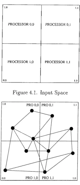
After modeling the tasks and processors,^ in order to apply the SOM al gorithm to find a mapping from ff'IG to PCG, the input and output spaces should be determined. We define S — [0 ,1]^ unit square to be the input space of our self-organizing map. We divide S into p regions (as shown in f ig ure 4.1 for p = 2 X 2) where p = Px x Py is the number of processors. Every

processor Pij has a region of coordinates, which is a subset of .5', bounded by

iX widths.., 7X widthy and (i + 1 ) x width^., (7 + 1 ) x widthy where widths. = l/p,,·

(29)

Solving the Mapping Problem with SOM

15

PROCESSOR 0,0

PROCESSOR 1,0

PROCESSOR 0,1

PROCESSOR 1,1

Figure 4.1. Input Space

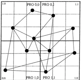
Figure 4.2. Input and Output Space

and widthy = l/z^i/· We define ta.sks to be the output space as neurons. The weight vectors of these neurons are selected to be positions on the unit square S like input vectors. That is, each weight vector, W = (x,y), and each input vector, / = (,'r, y) correspond to points in S. A task, i, is mapped to a processor

Pij if the weight of the neuron f, Wi, is in the region of Pij. Figure 4.2 shows a 4-processors space where some tasks are distributed over the processors.

Choosing TIG as output space means selecting the inputs from the unit square which represents the processors and organizing the tasks according to the selected input patterns. There is also another possibility: to select the TIG as input space and processor region (or processors) as output space [18] [19] [20],

(30)

16

but such a choice has some drawbacks which are explained by Quittek in de tail [22] .

initially all the tasks are randomly distributed over processor area. Then at ecxch successive step, weights of neurons evolve to cover the range of input space as follows:

1. Initialize all weight vectors, kk'°, randomly, (i.e., distribute tasks ran domly over processor area).

2. For t = 1 to tmax ■

(a) Select an input, P — (a;,?/) G S'.

Generally, uniformly distributed input selection (equal probability) models are used for SOM algorithms. This is the exact point where we force the algorithm to do load balancing. Rather than uniformly, we choose an input nearby the region of least loaded processor. Such a selection schema forces the algorithm to update the weight vectors of neurons to be close to the input, or in other words to the least loaded processor. Thus by this way, the load of the least loaded processor is increased. But on the other hand, how exactly the input P is chosen has an important impact on the performance of the algorithm. Should the input directly be chosen from the inside region of least loaded processor or should another method be used? In Chapter 5, we answer this question and discuss several alternative methods for selecting an input nearby the least loaded processor region. As a result of this analysis, we determine that' selecting the input directly from the region of the least processor performs best. (b) Determine excitation center c such that:

liv q -/‘ll = nijn||vq-/'

The input vector represents a coordinate information and it lies within the region of a processor area as mentioned in the above part. After the input is selected a neuron whose weight vector’s dif ference with the input is minimum should be determined. Since our

(31)

17

vectors determine a point in S, finding the excitation center corre sponds to finding the nearest neuron to the input in S. For a given input vector (coordinate) in order to find the closest neuron, all ver tices of TIG should be scanned beginning from the processor region that owns the input vector which is a very high-cost operation. In order to eliminate this drawback, we divide every processor region into grid connected subregions (Figure 4.3). By this way for a given input vector, in order to find the excitation center, beginning from the subregion that owns the input vector all surrounding subregions are scanned until the nearest neuron is found. This method is also known as “grid method” under the concept of range searching al gorithms in the literature. With this kind of an implementation we find the excitation center more quickly than the other way.

Figure 4.3. Subregions of processor regions (c) Update weights.

According to SOM algorithm we update the weight vectors of neu rons with:

^yt + l ^ pjyi ^ X ||/i _ p,/i||

where ||/* —kU/|| is the Euclidean distance between the weight vector of neuron i and input vector P.

Weight vector update section is the heart ol the algorithm. In the below section we take a closer look on the functions used in weight vector update.

(32)

18

i. Learning Rate Function: corresponds to the learning rate at time t. It determines the learning ratio of neurons at each step of the algorithm. Mostly it is a small value varying between i and 0. As Kohonen himself suggests [4] it may be any decreasing function with increasing time step. At the initial steps of the algorithm e is closer to 1, which means learning rate is high and neurons are highly affected from selected inputs. At later steps, as the value of it decreases so the learning rate ot neurons is and at final steps where e is closer to 0, the learning rate of neurons become minimal and only minor changes occur on weight vectors of neurons which also means the convergence of the algorithm. In our algorithm we use the below formula for e with 0.8 and 0.2 as initial and final values, which we decide to set after a few tests.

e* = epsilonlnitial x ( epsilonFinal ^ t

epsilon Initial tmax

2. Neighbourhood and Diameter; As we mentioned in Section 3.2, the di ameter function (i9) determines the neurons to be effected according to the selected input vector and it is generally embedded into the definition of neighbourhood function. It mainly defines the vicinity of input vector and is centered around the excitation center. Related to the definition of SOM algorithm and its biological background, the neurons in the vicinity of an input should be effected from the input, while the others should left intact. In our algorithm, the neurons to be effected from the input vector are the ones which are within 0 number of edges distant to the excitation center. In other words, if the number of edges on the shortest path between a neuron and the excitation center is less than or equal to

0 at that step, this means the neuron is in the vicinity of input vector and should be updated. Such a mechanism forms a way to preserve the topology and so neighbourhood relations.

Up to now, many different functions were used as neighbourhood diam eter function, in different applications. But the most common ones are, as Kohonen suggests [4], exponentially decreasing functions with respect to increasing time steps. In other words it is generally preferred to begin with a wide neighbourhood which makes all neurons effected from the input vector and so establishes a rough global order. At each successive

(33)

19

step, the diameter value decreases exponentially, where it becomes too small at final step and improves spatial resolution. However if the neigh bourhood is too small to start with, Kohonen says that the map will not be ordered globally,, rather mosaic-like parcellations would be seen. On the other hand if the neighbourhood is too large to start, unnecessary e.xecution time would be spent in order to have an ordered map. In our algorithm, we use the below function lor neighbourhood diameter where initial and final values are specified externally.

nt r 1 , the ta F in a P, t

0 — thetalmtial x (---— ) ' --- )

thetalnitial t,nax

Since the diameter function has a significant effect on the performance of the iilgorithm, its initial and final values should be determined carefully. In Chapter 6, we analyse the effect of variuos initial and final values in detail.

The point where neighbourhood diameter function, 0, effects the execu tion of SOM algorithm lies in the definition of neighbourhood function. Since only the neurons within the vicinity of the excitation center should be updated and others should be left intact, the neighbourhood function determines of rate the neurons in the vicinity should be effected from the current input pattern.

Schulten et. al [17] analysed the SOM algorithm from the point of con vergence and stability in detciil. According to their analysis for per fect ordering and stability the neighbourhood function should be convex, where they proved that concave neighbourhood functions always produce non-ordered maps. They also proved, under certain circumstances only Gaussian function produces acceptable results. Such circumstances in clude restrictions on neighbourhood diameter function, which we review in Chapter 6. The Gaussian neighbourhood function is also the one sug gested by Kohonen. The property that makes Gaussian a suita.ble choice is that it forces the neurons closer to excitation center highly eflected while the ones closer to the vicinity borders of an input vector less. In its Gaussian form, neighbourhood function(Figure 4.4) is generally lor- mulated as:

(34)

Solving the Mcipping Problem with

20

Figure 4.4. Gaussian Neighbourhood Function

0 outside neighbourhood (outside vicinity)

i^ ^ —d f c , ()

e within neighbourhood (inside vicinity)

where c/(c, i) is the number of edges in the output space between the neu ron i and excitation center c. So SOM cilgorithm recpiires the length of shortest path distances between excitation center and all other neurons. Since it is impossible to know which neurons would be selected as excita tion centers during the execution, we need to all shortest path distances between each pair of neurons. One way of obtaining this information is “all pairs shortest paths” algorithm which is applied by Heiss-Dormanss. Rather we design a simple algorithm which iteratively finds cind updates the weight vectors of neurons. That is, initially the excitation center is updated with distance 0. After that, the incident neighbours which are

distance + l far from the updated neuron are found and added to a queue. At each successive step one neuron is removed from the queue, updated and its nearest neighbours which are not updated are added to queue with necessary distance information until neighbourhood boundaries are reached. By this way we hnd and update the neurons in an ’’ expanding wave” manner efficiently.

As can be seen from the formula, neighbourhood function produces a maximum value, 1, for the excitation center (distance=0) and decreases exponentially with increasing distance from the excitcition center. So, ac cording to the definition of neighbourhood function the closer the neuron to excitation center, the higher the update ixitio.

(35)

21

According to weight update rule, two neurons which are awciy by same number of edges from excitation center at time t, have the same weight update ratio from the point of neighbourhood function. But since the formula contains the Euclidean difference ||/‘ - W^\\, the actual coordi nates of these neurons at time t, effect the ratio and the one which is more far away has a higher update ratio increasing with increasing Euclidean distance.

it is important to mention that during weight update, we do not take into account the communication loads of tasks. That is we do not apply a mechanism that updates the weight vectors of neurons according to some function of communication loads. Rather we prefer to use the orginal mechanism of SOM algorithm. However such a method is applied by Quittek which we discuss in Section 9.2 [21].

The definition and effect of neighbourhood function divides the execution of algorithm into two phases. The first phase can be ncimed as “ordering pha.se” . In this phase mainly the topological ordei'ing of weight vectors takes place. The second phase is “convergence phase” which is relatively much more longer than the former during which fine tunning of weight vectors is performed.

3. Number of Steps: Finally, we have to speak about the tmax parameter. According to Kohonen [4] for good statisticcil analysis ¿„xoi- value should be at least 500 times the number of neurons. But he also mention that for the tests he perform the number of steps do not exceed 100000 steps. This makes at most 200 nodes. On the other hand the test graphs used by researchers working on mapping generally have at least 10000 nodes. According to Kohonen this means 5000000 steps. But with such a param eter the execution of SOM, would probably take too much time. We think that the way Kohonen suggests the number ol steps possibly depends on perfect mapping. Because he also suggests that tor “fast learning” 10000 steps may be enough. For our problem we recdize that “fast learning” can be applicable, since we do not need an optimum solution for load balancing. A suboptimal solution within the 5% of the optimum solution is well accepted in many practical parallel applications. Of course the interprocessor communication should be kept low, but as we mentioned.

(36)

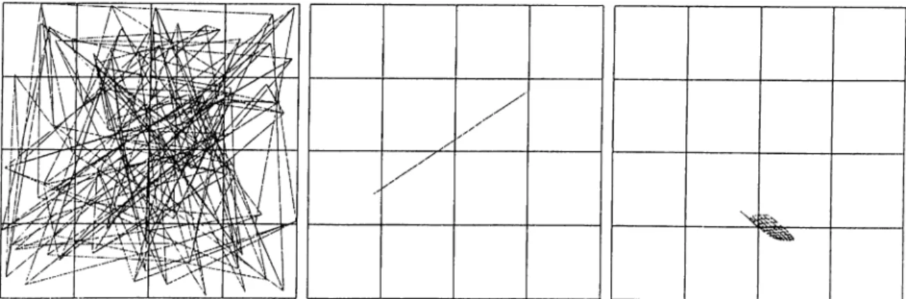
F'igure 4.5. E.xecution state.s for a .simple graph at steps 0, 50 and 400

Figure 4.6. Execution states for a simple graph at steps 3200, 5200 and 20000 reducing communication cost directly depends on neighbourhood preser vation, which SOM solves naturally. So more attention should be paid on load balancing. In order to satisfy equal load distribution the map may not be fully globally ordered. Rather a point in the “convergence phase” where the loads are nearly equally distributed is enough for us. Determining a number of steps value for each input TIG is meaningless and unnecessary. Rather we try to extract the number of steps value depending on the number of neurons. The analysis and its results can be found in Chapter 7.

In Figures 4.5 and 4.6, we represent a sanq^le execution ol our algorithm with an input graph of 100 nodes with grid connectivity. Initially, all the tasks are jxmdomly distributed over processor regions. Since the initial distribution is random, after 50 steps the vertices of the graph become closer which can be seen as preparation for further expands. The third figure represents the

(37)

23

situation at step 400. At step 3200 the graph began to e.xpand to fit the whole input space of processors. At step 5200, the graph represents the properties of input graph and it continues to e.xpand. The final figure shows the situation at step 20000 where all the vertices fit the proce.ssor area in a bcilanced load fashion.

(38)

Chapter 5 Study of Input Selection

In this chapter, we examine the impact of various input selection strategies on the ciccuracy of the algorithm. In order to test the performance of different methods we use most of the graphs listed in Table B-1 in Appendix B. For this analysis we perform assignments on 16 and 32 processors. Each execution in each test repeated 3 times for both 16 and 32 processors and average results are calculated and displa.yed. For each execution, we use uniformly distributed random numbers between 0 and 10 as computation and communication loads. The (speed of) processors and their communication liirk bandwidths are ac cepted to be identical. In Chapter 7, we discuss the effect of number of steps parcimeter so until that analysis we fix the number of steps value chcuiging between 5000 and 20000 according to the properties of input graphs.

For this and all other analysis in the rest of this thesis we use, the formulae given in Section 2.2 for load imbalance and communication cost calculation. VVe calculate execution time in seconds disccirding the time spent for input file reading. For input files we use Chaco format [29] [30] for compatibility purposes with other tools, since it is the most common used one. The Chaco file format is explained in Appendix A in detail.

Please note that just for the sake of display simplicity purposes, in some tables we abbreviate “Load Imbalance” as LI and “ Communication Cost” as “CC” or “ Comm. Cost” .

(39)

Study of Input Selection _2d

In the next section we present our alternative input selection methods and analyse their effect in Section 5.2.

5.1 Input Selection and Load Balancing

As we mentioned before, SOM algorithm satisfies the second requirement of mapping - neighbourhood preservation. That is Kohonen algorithm tries to place neighbouring neurons closer and this is exactly what a mapping should satisfy (placing neighbouring tasks closer). But there is the need to explic itly force the algorithm to take C cire of load imbalance. Generally, uniformly

distributed input selection models are used in SOM algorithms. This type of selection forces the SOM algorithm to distribute equal number of tasks to pro cessors without taking into account of task loads. But such a distribution is not a desired criteria for load balancing. So, SOM algorithm should be forced to distribute the loads of the tasks to processors in a balanced way. This can be achieved by selecting inputs from the regions closer to least loaded processor. By this way, such an input will probably force the algorithm to shift the tasks towards to least loaded processor which means assignment of more tasks to that processor, thus minimizing the load imbalance. During input selection, least loaded processor information can be directly used and an input within the region of the lecist loaded processor may be chosen or such an information can be used to determine another processor. In either case the possibility of selecting the least loaded processor should be high. A Gaussian distribution function identifying processor selection probabilities can be used as cin indirect method, still keeping in mind that least loaded processor has the maximum probability. Such a function usually chooses the least loaded processor or an other region closer to the least loaded with high probabilities, which satisfies our rec^uirements.

(40)

Study of Input Selection ₂₆

5.1.1 Processor Selection Strategies

VVe study the following alternative selection methods to determine the proces sor area for input selection;

• PRO-DLL: For this case, we directly select the input from the region of the least loaded processor.

• PRO-GASD: For this case, we select the input with high probability from the region of the least loaded processor. With decreasing probabil ities, the input is selected from neighbouring regions of the least loaded processors. In PRO-GASD strategy we define sets (or GASD levels) of processors around the least loaded processor. The first one of these sets is the least loaded processor. The next set contains the north,south, east and west neighbours of the least loaded processor. That is the ones that we can reach with one hop in any four directions (distance 1). The third set contains the ones that can be reached in two hops (distance 2) and so on as shown in Figure 5.1. The determination of GASD levels uses “edge- adjacency” strategy. In order to select a processor with this strategy, first of all, the processors which are in the same GASD level are determined and a probability value is assigned to each level according to Gaussian distribution function, where the least loaded processor has the maximum probability. Afterwards, one of the processors in the determined GASD level is selected with uniform probability.

□

Least Loaded Processor I [ Distance 5 Cells r . ' Distance 4 Cells

Distance 3 Cells Distance 2 Cells Distance 1 Cells

Figure 5.1. Subregion selection by “ Gaussian Distribution with Distance In formation”

(41)

Study of Input Selection

27

• PRO-GASR: This method is very similar to PRO-GASD. The only differ ence with PRO-GASD is the definition of levels. Here during the deter mination of GASR levels both “edge-adjacency” and “corner-adjacency” strategies are used as shown in Figure 5.2.

□

Least Loaded Processor

I I Levels Cells

Level 2 Cells Level 1 Cells

Figure 5.2. Subregion selection by “ Gaussian Distribution with Region Infor mation”

After we determine the processor region we need to determine an input vector within that region. The next section discusses alternative ways to select the input.

5.1.2 Subregion Selection Strategies

For fast computation of determining the nearest neuron to an input, the proces sor regions are divided into subregions. Following the similiar strategies that we apply for processor selection, we try different methods to select a region within the processor than an input within the region.

VVe apply the same functions used for processor selection. But since least loaded .selection is not as important as in processor selection for subregions from the point of load imbalance, we also test two other alternative methods which are “ Uniform” and “ Center” which are explained below.

Center (Cent): In this case, we directly choose the subregion in the cen ter of the processor region. In the case of even number of subregions

(42)

28

existance, there would be four subregions in the center. This time, we select one ot the four subregions randomly.

• Uniform (Uni): A uniformly distributed random number is used to de termine the subregion.

• Least Loaded (Dll): For this strategy the subregion whose load is mini mum within the determined processor is selected.

• Gaussian with Distance (Gasd): This is the same method as PRO-GASD applied for subregions within the selected processor region.

• Gaussian with Region (Gasr): This is the same method as PRO-GASR applied for subregions within the selected processor region.

5.2 Effect of Input Selection Strategies on Load

Balance

In order to determine the most suitable processor and subregion for input selection, we test all subregion selection strategies for each processor selection strcitegy with all other parameters fixed.

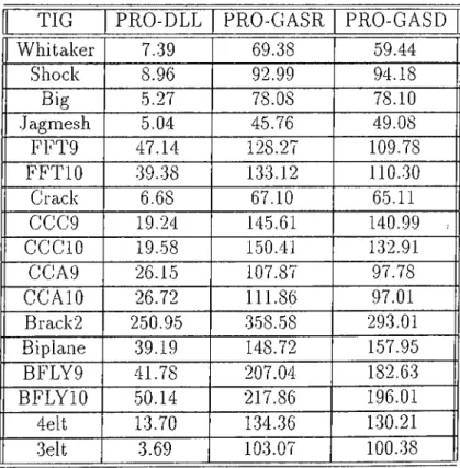
In Tables 5.1 and 5.2, we present the load imbalance values for the three processor selection strategies on 16 and 32 processors respectively. For the sake of display simplicity the tables do not include subregion selection strate gies. Rather we take average values of five subregion selection strategies for each graph and processor selection strategy. What we have is an average load imbalance related to each processor selection strategy.

According to the tables it is clear that for both 16 and 32 processors PRO- DLL outperforms the other methods PRO-GASR and PRO-GASD Irorn the point load imbalance lor all input graphs. So, we select PRO-DLL as processor selection strategy. That is forcing SOM algorithm to select the inputs always from the least loaded processor enables distributing the loads in a more bal anced fashion. Now we go one step further and analyse the subregion selection strategies with PRO-DLL as a processor selection strategy.

(43)

29

TIG PRO-DLL PRO-GASR PRO-GAS D Whitaker 0.99 45.38 36.70 Shock 0.58 50.52 50.62 Big 0.47 33.21 33.98 .Jagmesh 2.42 14.26 22.63 FFT9 10.28 74.09 61.56 FFTIO 13.54 79.96 55.41 Crack 1.01 36.05 .33.02 CCC9 13..39 107.43 92.42 CCCIO 21.12 121.31 98.73 CCA9 4.76 r 82.14 58.01 CCAIO 10.62 86.12 63.67 Brack2 64.56 129.09 144.80 Biplane 2.44 74.47 67.09 BFLY9 44.13 148.89 127.99 BFLYIO 54.18 123.58 156.53 4elt 0.80 69.95 64.68 3elt 0.56 54.43 52.16 Table 5.1. Load Imbalance results for 16 processors(%)

TIG PRO-DLL PRO-GASR PRO-GASD Whitaker 7.39 69.38 59.44 Shock 8.96 92.99 94.18 Big 5.27 78.08 78.10 Jagmesh 5.04 45.76 49.08 FFT9 47.14 128.27 109.78 FFTIO 39.38 133.12 110.30 Crack 6.68 67.10 65.11 CCC9 19.24 145.61 140.99 : CCCIO 19.58 150.41 132.91 CCA9 26.15 107.87 97.78 CCAIO 26.72 111.86 97.01 Brack2 250.95 •358.58 293.01 Biplane 39.19 148.72 157.95 BFLY9 41.78 207.04 182.63 BFLYIO 50.14 217.86 196.01 4elt 13.70 1.34..36 130.21 3elt 3.69 103.07 100.38

(44)

30

In Tables 5.3, 5.4, 5.5 and 5.6, we give execution results related to PRO- DLL for both five subregion selection strategies. Tables 5.3 and 5.4 correspond to execution results for 16 processors for load imbalance and communication cost respectively. The values displayed in Tables 5.5 and 5.6 organized in the same manner to represent the execution results for 32 processors.

When the values in the tables are analysed it can be seen that it is really hard to determine the best subregion selection strategy. So the values are analysed in another way. Since in SOM algorithm the connection schema of neurons are important, we group the results according to types of graphs. That is we calculate an average value for graphs of the same class. Since we have seven different class of input graphs for this analysis, we obtain seven values for each subregion selection strategy. The Tables 5.7 - 5.8 and 5.9 - 5.10 present these grouped average values for 16 and 32 processors respectively. The first ones in each pair present load imbalance results where second ones present communication cost results.

Before commenting on the grouped values according to graph type, one point should be mentioned that we are searching a method which shows best performance on the average for all graph types. It is not a desired criteria that a method performs best for one graph and/or graph class and worst for any other. Additionally since SOM works probably better for geometric graphs, the method we choose should i^erforrn well for graph types like Grid or FEM too. In order to easily comment on results we calculate the number of times that these strategies found maximum and minimum values. According to this calculation from the point of load imbalance; •

• Cent found 7 rninimums and 10 maximums, • Dll found 10 minimums and 5 maximums, • Uni found 7 minimums and 12 maximums, • Gasd found 7 minimums and 3 maximums. Gasr found 3 minimums and 4 maximums.

(45)

31

Subregion Selection Strategies Graph Cent Dll Uni Gas cl Gasr Whitaker 0.90 0.59 0.61 1.05 1.82 Shock 0.46 0.67 0.17 1.38 0.24 Big 0.84 0.60 0.12 0.35 0.45 Jagmesh 2.28 2.13 2.42 3.03 2.23 FFT9 1.44 19.32 6.44 4..38 19.85 FFTIO 24.98 17.54 5.63 10.60 8.96 Crack 2.30 0.85 0.86 0..35 0.69 CCC9 14.17 3.99 24.05 12.72 12.03 CCCIO 20.88 12.23 41.17 19.06 12.27 CCA9 0.67 2.54 15.97 1.74 2.87 CCAIO 6.66 9.24 23.62 10..32 3.26 Brack2 116.83 28.33 64.93 46.49 66.20 Biplane 3.53 1.71 2.93 0.79 3.26 BFLY9 53.87 17.05 67.83 49.63 32.24 BFLYIO 63.11 16.95 73.33 58.84 •58.67 4elt 0.83 0.36 1.80 0.27 0.75 3elt 0.59 0.58 0.73 0.44 0.48

Table 5.3. Load Imbalance results for PRO-DLL (%)(16 processors) Subregion Selection Strcitegies

Graph Cent Dll Uni Gasd Gasr Whitaker 0.79 0.78 0.75 0.79 0.75 Shock 1.47 1.58 1.53 1.68 1..59 Big 0.97 0.98 0.91 0.92 0.96 .Jagmesh 0.19 0.20 0.18 0.19 0.20 FFT9 2.27 2.39 2.07 2.14 2.11 FFTIO 4.74 5.11 4.22 4.64 4..54 Crack 0.86 0.84 0.77 0.76 0.79 CCC9 1.97 2.01 1.88 1.90 1.98 CCCTO 4..34 4.39 4.07 4.18 4.28 CCA9 1.32 1.27 1.25 1.22 1.18 CCAIO 2.80 2.80 2.76 2.61 2.69 Brack2 20.78 23.63 18.31 18.62 19.73 Biplane 1.02 1.20 1.09 1.22 1.09 BFLY9 3.88 3.82 3..53 3..53 3.64 BFLYIO 8.14 8.50 7.68 7.88 8.06 4elt 0.97 1.23 1.09 1.05 1.14 3elt 0.48 0.63 0..52 0.56 0.56

Table 5.4. C

j (xl0000)(16 processors)

(46)

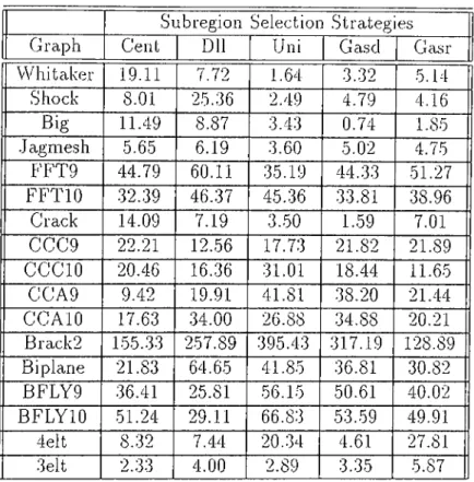
32

Subregion Selection Strategies Graph Cent Dll Uni Gas cl Gasr VVhitake.r 19.11 7.72 1.64 3.32 5.14 Shock 8.01 25.36 2.49 4.79 4.16 Big 11.49 8.87 3.43 0.74 1.85 .Jagmesh 5.65 6.19 3.60 5.02 4.75 FFT9 44.79 60.11 35.19 44.33 51.27 FFTIO .32.39 46.37 45.36 33.81 38.96 Crack 14.09 7.19 3.50 1.59 7.01 CCC9 22.21 12.56 17.73 21.82 21.89 CCCIO 20.46 16.36 31.01 18.44 11.65 CCA9 9.42 19.91 41.81 38.20 21.44 CCAIO 17.63 34.00 26.88 34.88 20.21 Brack2 L55..33 257.89 395.43 317.19 128.89 Biplane 21.83 64.65 41.85 36.81 30.82 BFLY9 36.41 25.81 56.15 50.61 40.02 BFLYIO 51.24 29.11 66.83 53.59 49.91 4elt 8.32 7.44 20.34 4.61 27.81 3elt 2.33 4.00 2.89 3.35 5.87

Table 5.5. Load Imbalance results for PRO-DLL (%)(32 processors) Subregion Selection Strategies

Graph Cent Dll Uni Gascl Gasr Whitaker 1.04 1.06 1.02 1.02 1.02 Shock 2.00 2.41 2.11 2.18 2.21 Big 1.80 1.62 1.42 1.43 1.39 .Jagmesh 0.31 0.36 0.32 0.31 0.31 FFT9 3.62 3.91 3.37 3.31 3.45 FFTIO 7.38 7.76 6.73 7.23 7.41 CRACK 1.33 1.30 1.26 1..30 1.29 CCC9 3.16 3.24 2.94 3.01 2.95 CCCIO 6.97 6.86 6.46 6.46 6.49 CCA9 2.14 2.13 1.94 1.95 1.92 CCAIO 4.70 4.49 4.19 4.09 4.06 Brack2 34.30 31.06 27.51 29.50 32.57 Biplane 1.97 1.88 1.87 1.81 1.86 BFLY9 6.23 6.25 5.44 5.85 5.75 BFLYIO 13.71 13.93 12.28 12.21 12.75 4elt 1.67 1.94 1.72 1.67 1.78 3elt 0.81 1.01 0.85 0.81 0.88

(47)

33

Subregion Selection Strategies Graph Cent Dll Uni Gasd Gasr FEM(2) 1.09 0.60 0.82 0.49 0.84 FEM(3) 116.83 28.33 64.93 46.49 66.20 HB 2.28 2.13 2.42 3.03 2.23 Butterfly 35.85 17.71 38.31 30.86 29.93 CCC 17..53 8.11 32.61 15.89 12.15 Grid 2.00 1.19 1..55 1.08 1.75 CCA 3.67 5.89 19.79 6.03 3.07

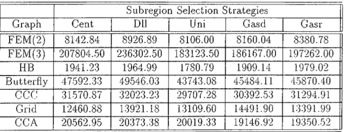
Table 5.7. Grouped Load Imbalance results for PRO-DLL (%)(16 processors) Subregion Selection Strategies

Graph Cent Dll Uni Gasd Gasr FEM(2) 8142.84 8926.89 8106.00 8160.04 8380.78 FEM(3) 207804.50 236302.50 183123.50 186167.00 197262.00 HB 1941.23 1964.99 1780.79 1909.14 1979.02 Butterfly 47592.33 49.546.03 43743.08 4.5484.11 45870.40 CCC 31570.87 32023.23 29707.28 30392.53 31294.91 Grid 12460.88 13921.18 13109.60 14491.90 13391.99 CCA 20562.95 20.373.38 20019.33 19146.92 193.50..52 Table 5.8. Grouped Cornmuniccition Cost results for PRO-DLL (16 processors)

According to average values and number of minimums and maximums we can easily eliminiite “ Cent” and “Uniform” . When we take into account num ber of maximums, we see that “Dll” produced 7 minimums and 0 mciximurns for 16 processors. However it produces 3 minimums and 5 maximums for 32 processors. So, increasing number of processors significantly effects the per formance of “ Dll” . Although it performs best for 16 proces.sors, it is also one of the worst methods for 32 processors. So we can cilso eliminate the “ DU” strategy. What left is the strategies depend on Gaussian formulation. The load imbalance values produced with these methods look close except tor the one produced for “ Brack2” lor 32 processors. It we omit load imbalance results of “Brack2” and consider them as exceptional cases, the sum ot load imbalance values for these two methods become “221.417” and “226.273” tor 16 processors and “355.908” and “.342.770” for 32 processors. If we just take into account

(48)

Study ot Input Selection

34

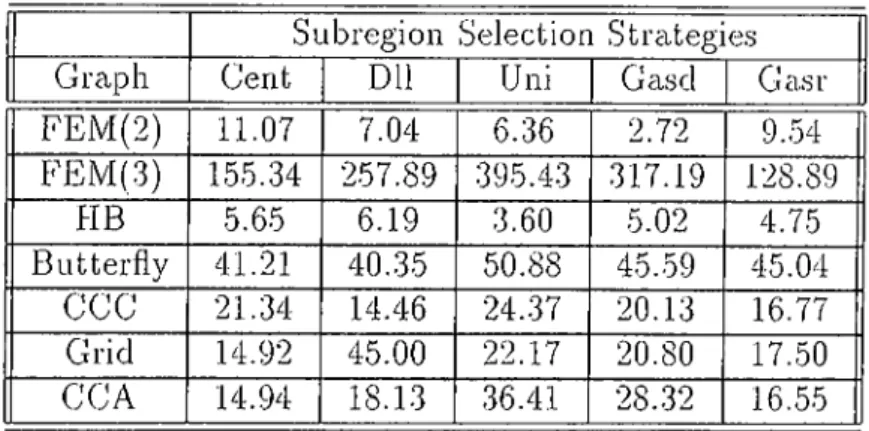
Subregion Selection Strategies Graph Cent Dll Uni Gasd GclSr FEM(2) 11.07 7.04 6.36 2.72 9..54 FEM(3) 155.34 257.89 395.43 317.19 128.89 PIB 5.65 6.19 3.60 5.02 4.75 Butterfly 41.21 40..35 50.88 45.-59 45.04 CGC 21.34 14.46 24.37 20.13 16.77 Grid 14.92 45.00 22.17 20.80 17.50 CCA 14.94 18.13 .36.41 28..32 16.55

Table 5.9. Grouped Load Imbalance re.sult.s for PRO-DLL (%)(32 proces.sor.s) Subregion Selection Strategie.s

Graph Cent Dll Uni Gasd Gasr FEM(2) 13293.47 13856.63 12537.14 12451.75 12729.07 FEM(3) 342950.50 310561.00 275089.50 295047.50 325701..50 HB 1941.23 1964.99 1780.79 1909.14 1979.02 Butterfly 77.352.45 79640.28 69569.68 71489.23 7.3411..57 CGC 50667.32 .50516.83 47031.46 47335.08 47218.57 Grid 19829.66 21482.67 19928.47 19944.07 20374.64 CCA 34178.73 33103.57 30636.82 30192.63 29899.68 Table 5.10. Grouped Communication Cost results for PRO-DLL (32 proces sors)

these values although they are really close, it seems that “Gasr” is better. But if we also take into account the calculations related to minimums and maxi mums, since “ Gasd” produced more minimums and less maximums and since the average load imbalance values are close we prefer “ Gasd” as the subregion selection strategy.

Choosing the best subregion selection method is not as straightforward ¿is proces.sor selection. But it seems “ Gasd” performs better. That is, the values are not best all the time, but on the average this method produces stable results. For all graph types and processor selection strategies, the maximum load imbalance value produced by this method is 58%, while all other methods produced at least one value over 64%. As a result PRO-DLL combined with “ Gasd” subregion selection strategy distributes loads more balanced than the

(49)

35

other combinations. So for the analysis hereafter we use “ PRO-DLL, Glasd” pair for input selection.

(50)

Chapter 6 Impact of Neighbourhood

Diameter on Load Balance

In this chapter, we examine the impact of neighbourhood diameter function on the accuracy of the algorithm. In order to test different diameter values we use test graphs selected from the list in Table B-1 in Appendix B. I'or this analysis we perform assignments on 16 and 32 processors. Each e.xecution in each test repeated 3 times for both 16 and 32 processors and average results are calculated and displayed. For each execution, we use unilormly distributed random numbers between 0 and 10 as computation and communication loads. The (speed of) processors сшс1 their communication link bciridwidths cire ac cepted to be identical. In Chapter 7, we discuss the effect of number of steps parameter, so within this section we fix the number of steps value changing between 5000 and 20000 according to the properties of input grciphs.

.As we mentioned in Chapter 4, specicil attention should be paid on neigh bourhood diameter function’s initial cind final values. Schulten et. al [17] advice that the initial value of 9 should be in the orders of number of neurons. Koho- nen advices the initial value of 9 should be larger than the half of the diameter of the output spcice [4]. He also advices the final value of 9 should be equal to unit distance in order to include just the nearest neighbours of excitation center for finer refinements. In a similar implementation [18] Heiss-Dormanns use and 0.45 as initial and final values respectively. On the

A new load balancing heuristic using self-organizing maps

A NEW LOAD BALANCING HEURISTIC USING

SELF-ORGANIZING MAPS

A THESIS

SUBMITTED TO THE DEPARTMENT OF COMPUTER

ENGINEERING AND INFORMATION SCIENCE

AND THE INSTITUTE OF ENGINEERING AND SCIENCE

OF BILKENT UNIVERSITY

IN PARTIAL FULFILLMENT OF THE REQUIREMENTS

FOR THE DEGREE OF

MASTER OF SCIENCE

By

Murat Atım

September, 1999

ABSTRACT

A NEW LOAD BALANCING HEURISTIC USING

SELF-ORGANIZING MAPS

Murat Atun

M. S. in Computer Engineering and Information Science

Supervisor: Asst. Prof. Attila Gürsoy

September, 1999

ÖZET

KENDİNDEN DÜZENLENEN HARİTALAR ALGORİTMASI

KULLANAN YENİ BİR SEZGİSEL YÜK DENGELEME

ALGORİTMASI

Murat Atım

Bilgisayar ve Enformatik Mühendisliği Bölümü Yüksek Lisans

Tez Yöneticisi; Yrd. Doç. Attila Gürsoy

Eylül, 1999

Acknowledgement

Contents

List of Figures

List of Tables

Chapter 1

Introduction

Chapter 2

Mapping Problem

2.1

Mapping

2.2

Models for Representing Processors and

Tasks

6

Chapter 3

Kohonen SOM

3.1

Biological Background

10

3.2

Algorithm

11

12

/

/

///

•

\

////

/

\\\\

Excitatio

Center

'\

Input

(c)

Chapter 4

Solving the Mapping Problem

with SOM

15

16

liv q -/‘ll = nijn||vq-/'

17

18

19

20

21

23

Chapter 5

Study of Input Selection

5.1