GPU-Based FFT Computation for Multi-Gigabit WirelessHD Baseband Processing
Tam metin
Şekil


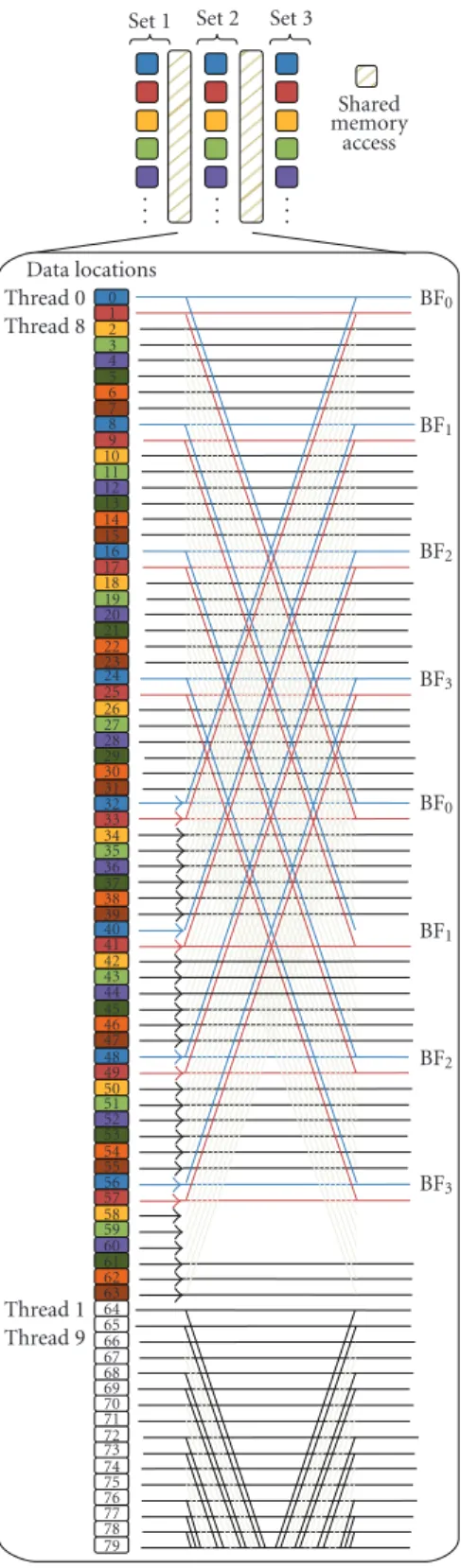

![Figure 13: The CUDA FFT code [ 24 ] with explanation of its execution.](https://thumb-eu.123doks.com/thumbv2/9libnet/3618869.21239/11.900.83.821.88.1077/figure-cuda-fft-code-explanation-execution.webp)
Benzer Belgeler
Çakmak taşından yapılmış âletlere gelince, büyük eklalarla muttasıf Musteriyen aletlerini,ekseriya uzun ve dar ve çok ince işlenmiş olan lam tekniği takip
In order to estimate the nominal subsidy rates in the tradeable sectors of the Turkish economy, we first consider the sum total of sectoral subsidies
sion in the previously published large signal equivalent cir- cuit model for a circular capacitive micromachined ultrasonic transducer (CMUT) cell.. The force model is rederived
[r]
Kad›n tarihi ya da feminist tarih alan›nda Bat›l› tarihçilerin yapt›klar› çal›flmalar, ta- rihe kaydedilmemifl dolay›s›yla tarihyaz›m›na konu olmam›fl ve
Güven Bölgeleri ve Kitle Ortalama Vektörünün Bileşenlerinin Eşanlı Karşılaştırılması Çok değişkenli bir örneklemden sonuç çıkarımı yapmak için, tek
A nearly crack-free surface was achieved on sample B with a 700 nm AlGaN graded interlayer and 400 nm HT-AlN layers GaN grown on the silicon substrate.. This indicates that the
Using this technique, we have cut the number of intermediate frames by half and re-generated them using image morphing during the rendering phase to save an extra space from
