A multi-objective and multi-period model to design a strategic development program for biodiesel fuels

(1)

Contents lists available atScienceDirect

Sustainable Energy Technologies and Assessments

journal homepage:www.elsevier.com/locate/seta

A multi-objective and multi-period model to design a strategic development

program for biodiesel fuels

Ramin Hosseinalizadeh

a

, Alireza Arshadi Khamseh

b,⁎

, Mohammad Mahdi Akhlaghi

c

a_{Industrial Engineering Department, Faculty of Engineering, Kharazmi University, Tehran, Iran}

b_{Associate Professor Department of International Logistics and Transportation, Faculty of Economics Administration and Social Sciences, Istanbul Gelisim University,} Turkey

c_{Niroo Research Institute, Renewable Energy Department, Tehran, Iran}

A R T I C L E I N F O Keywords: Biodiesel Supply chain Development planning Environmental eﬀects A B S T R A C T

The air pollution of conventional fuels, increases the tendency to alternative cleaner fuels like biodiesel fuels. Biodiesel is an expensive fuel and can be used as an additive to reduce levels of particulates, carbon monoxide, and other pollutants released from diesel fuel. The proportion of biodiesel in the produced fuel can be planned and controlled according to the conditions. This study forms a comprehensive multi-objective-period model for designing a biodiesel development program and compares different biodiesel blends and primary resources. The study considers B5, B10, B20, B40, and B100 along with diesel as the candidate fuels for demand fulfillment; furthermore, model considers waste cooking oil, soya, sunflower, and rapeseed as the primary resources. The objectives are the facilities' implementation costs and environmental effects minimization. The decision vari-ables are the capacity planning and the facility location varivari-ables. The exact Pareto set is obtained by using the augmented e-constraint method. The study considers economic and environment objectives interactions. Based on the results, B5 and B40 are the most appropriate options in the exact Pareto set; moreover, the results show the advantages of this approach to select the most appropriate fuels and primary resources according to different conditions during the studied period.

Introduction and literature review

Due to the value of non-energy uses of fossil fuel products in in-dustries (for example petrochemical inin-dustries that produce various and valuable products by reforming methane and propane) along with the high price of crude oil and global environmental problems, focusing on new energy resources have been increasing across the world. Moreover, the air pollution of fossil fuels, especially in urban areas, raises the tendency to alternative fuels such as biodiesel. Biodiesel can be used as a fuel in the pure form; however, due to its cost, it is usually used as a diesel additive to reduce levels of particulates, carbon monoxide, and hydrocarbons derived from diesel-powered vehicles [1]. The use of biodiesel-diesel blends in CI engines has been proven to lead to a great decrease in particulate matter, hydrocarbon, and carbon monoxide compared to diesel fuel. There are diﬀerent ideas about nitrogen oxides. Some researches show an increase [2], and some others show a de-crease in the quantity of nitrogen oxide [3]. Many researches were conducted on the life cycle assessment (LCA) of biofuels to specify the environmental impacts of them and compare them with conventional

fuels[4–7]. Altamirano et al.[8]tracked CO2 emissions, energy e ﬃ-ciency, water and resources consumption, and environmental impacts of two biodiesel production chains.

Biodiesel is produced using transesterification. Feedstocks for bio-diesel include animal fats, vegetable oils, soy, rapeseed, jatropha, sunflower, palm oil, field pennycress, algae, waste cooking oil, etc. Thus, biofuel is a renewable fuel since its feedstocks are always avail-able;

Furthermore, some of the feedstocks are municipal, industrial, or agriculture waste. Therefore, using these feedstocks for producing biofuel, in addition to reducing pollution, also helps to manage wastes. Cambero et al.[9]and Zhong et al.[10]considered some social and environmental advantages of bioenergy and biofuel supply chains.

In recent years, the biofuel industry has become complicated which make it increasingly diﬃcult to be analyzed and optimized[11]. The high cost of such fuels restricts their application; an approach to dealing with this problem is studying and optimizing their supply chains. For this purpose, many studies were carried out that consider diﬀerent as-pects. Ghaderi et al.[12]reviewed 146 papers on the supply chains of

https://doi.org/10.1016/j.seta.2019.100545

Received 27 December 2018; Received in revised form 26 August 2019; Accepted 12 September 2019 ⁎_{Corresponding author.}

E-mail addresses:Ramin.h_alizadeh@yahoo.com(R. Hosseinalizadeh),akhamseh@gelisim.edu.tr(A. Arshadi Khamseh),Makhlaghi@nri.ac.ir(M.M. Akhlaghi).

(2)

the biomass-based energy systems. Furthermore, Atashbar et al.[13] present a classiﬁcation of optimization methods and models developed for biomass supply chains.

An economic model was developed by Whalley et al.[14]to esti-mate the delivery cost of biomass chips to a biorefinery. Zhang et al. [15]developed a new multi-agent feedstock supply model specifically for China. Senna et al. [16]presented a comparison between a two-stage model and a multitwo-stage stochastic model to optimize the biodiesel supply chain. Golecha et al. [17]suggested a cost model for biomass transportation from afield to a conversion facility. Hao Hu et al.[18] have considered a cyber GIS approach to optimize biomass supply chains under uncertainties. A mathematical model was presented by Mirkouei et al.[19]for determining the optimal combination and lo-cation of refineries for a known quantity of woody biomass. An RDEA-based algorithm was proposed by Grigoroudis et al.[20]for the optimal design of supply chain networks. Ivanov et al.[21]addressed the op-timal design and location facility of biodiesel supply chains under economic and environmental criteria. Azadeh et al.[22]analyzed the challenges of supplying biomass to biorefineries and shipping biofuel to demand centers. Yazan et al.[23]compared different second-genera-tion biomass supply chain designs focusing on mobile pyrolysis plants and centralized versus a decentralized collection of biomass regarding economic and environmental sustainability. Osorio-Tejada et al.[24] compared biodiesel and liquefied natural gas as alternative fuels in transport systems. A stochastic bi-objective Mixed Integer Problem model was presented by Cáceres[25]to optimize biodiesel supply chain networks.

Some other studies considered similar subjects in other areas. For example, the grid design and optimal allocation of wind and biomass resources for renewable electricity supply chains are studied by Osmani et al.[26]. Tan et al.[27]focused on the fuel supply chain of biomass direct-fired power generation. Their objectives comprise profit and social welfare maximization. Xiaojing et al.[28]studied improving the efficiency of biogas feedback supply chain. Woo et al.[29]presented a new optimization-based approach for the design and operation of a renewable hydrogen system from various types of biomass. Moreover a similar study was carried out by Guillén et al.[30]. They addressed the design of hydrogen supply chains for vehicle use with economic and environmental concerns. Jeong et al.[31]developed a mixed-integer linear programming model associated with a geographic information system to optimize a supply chain for biodiesel produced from camelina oilseed.

Laporte et al. [32] assessed the supply of switchgrass and mis-canthus in Canada, under different biomass prices and supply chain structures, using an integrated economic, biophysical and GIS model, to assess bioenergy policy. Lainez-Aguirre et al.[33]presented aflexible supply chain superstructure to deal with issues on economic and en-vironmental benefits achievable by integrating biomass-coal plants, and CO2capture and utilization plants.

Table 1shows a review of some other related works carried out in recent years. Most of these researches selected just one fuel such as B5 and studied its economic, environmental, or technical aspects. But it is important why the fuel is selected, and which fuel is the best according to the conditions. Since biodiesel can be used as an additive to con-ventional fuels and the share of it in the new fuel is effective on the released pollution, the volume of required biodiesel, and the cost of the new fuel, it is necessary to know which fuel and when should be pro-duced. It might be possible and effective to use several biodiesel blends simultaneously in different periods instead of using only one fuel. This can lead to a decrease in costs and can help the government to accel-erate the development of these kinds of fuels. These studies haven’t discussed this statement and have failed to suggest development plans for these kinds of fuels. This study aims to propose a mathematical framework to investigate the best blends of biodiesel fuel. In the fol-lowing, the contribution of the paper has been demonstrated in detail. Considering the high cost of biodiesel, it seems that the blends of

biodiesel and conventional hydrocarbon-based diesel could be more economical since the cost is an obstacle in the way of widespread use of these fuels. Therefore, these blends (B40, B20, B10, and B5) are the most common fuels in the retail diesel fuel market and have different price and released pollutant. Mentioned studies have focused on various aspects of biofuels supply chains. Primary resources, produced fuels, and objectives are different among the studies. As mentioned, most of the related researches investigate solely one fuel or consider only one resource as a feedstock which may not be optimum. On the other hand, it is difficult to choose the best biodiesel blends and resources among the candidates. Therefore, in this study, a comprehensive multi-objec-tive and multi-period MIP model is proposed to compare these fuels and select one or more of them to fulfill fuel demand in the study period. This model also suggests the best primary resources for each year of the studied period.

The proposed biofuel supply chain includes different facilities such as oil extraction plants, waste oil refineries, biodiesel and fuel blending plants and different products such as biodiesel blends and glycerin as well. For this purpose, B5, B10, B20, B40, and B100 are considered as the candidate blends and waste cooking oil, soya, sunflower, and ra-peseed as the primary resources. Based on the results of this model, the capacity of facilities will be determined in the model’s horizon. Furthermore, the type of fuels that the decision-makers should con-centrate on will be chosen. This information can be used for designing a development plan for biodiesel fuels in countries and big cities.

The rest of this paper consists of two main sections. In theﬁrst section, the model is described. This section discusses the proposed supply chain and then presents the mathematical model’s objectives and constraints, respectively. The results obtained after running the model for a case study are presented in the second section. In this section, the results of the running and some sensitivity analyses for some parameters are brought in the form of several trends, tables, and ﬁgures.

Model

Proposed supply chain

Different kinds of crops are suitable as a primary resource for pro-ducing biodiesel. The proposed model considers waste cooking oil and three crops, namely soya, sunflower, and rapeseed. The oil of crops is extracted in extraction plants, and the waste cooking oil is refined in waste oil refineries. Then, they are transported to biodiesel refineries and transformed into biodiesel and glycerin. Biodiesel and glycerin are produced according to the transesterification process as shown below [34].

+ → +

Oil Methanol Biodiesel Glycerin (1)

Next, produced glycerin is transported to glycerin distributor and then to glycerin demand centers. Additionally, the produced biodiesel is delivered to blending plants along with diesel fuel; in each candidate region, all biodiesel blends, namely B5, B10, B20, B40, and B100 can be produced. Afterward, these fuels are sent to demand centers. Furthermore, the proposed model considers the import of oil, biodiesel, and crops from outside of the study area.Fig. 1shows the diagram of this process.

Some factors like cetane number, oxidation stability, iodine number are necessary for blending diesel and biodiesel from diﬀerent sources. However, this study ignores them because of simpliﬁcation.

Mathematical model

This section explains the mathematical model of the proposed supply chain. First, the objective functions, and then, the constraints are mentioned.Table 2shows the nomenclature of the model.

(3)

Table 1 Literature review. Ref Year Subject Resource Fuel Model & Solving method [42] 2018 Environmental and techno-economic considerations Frying oil Biodiesel – [43] 2018 Techno-economic analysis Palm oil Biodiesel Techno-economic analysis Simulation [44] 2018 design biodiesel supply chain Jatropha, waste oil cooking and microalgae biodiesel MILP [45] 2018 Scale-up and economic analysis Recycled grease trap waste Biodiesel Economic feasibility Simulation [11] 2017 To quantify and control the impact of biomass quality variability on supply chain related decisions and technology selection Biomass Biofuel An L-shaped and a multicut L-shaped method [46] 2017 To design a sustainable multi-period supply chain 2th generation biomass Bioethanol Augmented ε-constraint method [47] 2017 The strategic design of biodiesel supply chain network Jatropha, curcas, waste cooking oil Biodiesel DEA & MILP [48] 2017 Supply chain network design Jatropha seeds, waste cooking oil Biodiesel MILP [49] 2017 Finding the optimal production and investment plan for a biogas supply chain Straw, sugar beet and manure Natural gas, heat, and electricity MIP [50] 2017 A novel biore fi nery concept for lignocellulosic biomass Black liquor, Sawdust, Straw Biofuel – [51] 2017 The fuel supply chain of biomass direct-fi red power generation Biomass Biomass – [52] 2016 An Overview on Production, Properties, Performance and Emission Analysis – B20, B100, E10, M10 Overview [53] 2016 Proposing a sustainable supply chain model capable of revealing opportunities and limitations Microalgae Biofuel biofuel [54] 2016 Design and plan a supply chain from fi elds to consumption markets Biomass Biodiesel System dynamics-MIP [55] 2016 Locating biofuel facilities and designing a supply chain to minimize the overall cost Woody biomass Biofuel MILP [56] 2016 A two-stage model for the design and planning of a microalgae-based supply chain. Microalgae Biodiesel Robust mixed-integer linear programming [57] 2016 The optimal design of supply chains considering all policy instruments of European regulations. Lignocellulosic biomass Biofuel – [58] 2016 Maximizing the supply chain of a forest-based biomass power plant Forest-based biomass electricity MILP-Robust optimization [59] 2016 An optimization by considering all the dimension of the sustainable development 1th and 2th generation biomass Bio-ethanol MILP [60] 2016 the design of an integrated biodiesel-petroleum diesel blends system sun fl ower, rape and other oil seed crops B100 MILP [39] 2016 The performance and emission of diesel engine with soybean and waste oil biodiesel fuels – B5, B10, B15, B20 and B50 Experiment [61] 2015 Studying of the optimal conditions of the supply chain biodiesel via the techno-economic and environmental analysis. Oil palm crop B20 MOMILP [40] 2015 Eff ect of di ff erent percentages of biodiesel –diesel blends on a diesel engine – B5, B10, B15, B20, B25, B50 and B100 Experiment [62] 2015 the best biodiesel blend selection – B20, B40, B60, B80, B100 and Diesel MCDM [63] 2015 Strategic planning design of a supply chain network Microalgae Biodiesel MILP [64] 2015 Supply chain design and planning for biomass to electricity Residual forestry biomass Bioelectricity MILP [65] 2015 Determine the optimal supply chain design and operation, under uncertainty. Wastes or lignocellulosic feedstocks Biofuel MILP [66] 2014 A life cycle assessment (LCA) based supply chain model Biomass Bio-ethanol, Bio-methanol, Bio-diesel MOMILP [67] 2014 Analyzing of The production chain of biofuels from agricultural residues Agricultural residues Biofuel MILP This study To design a strategic development program Waste cooking oil, Soya, Sun fl ower, and Rapeseed B5, B10, B20, B40, B100 MOMILP

(4)

Farms

Waste cooking oil production

centers

Oil collectors & producers Waste oil refineries BioDiesel refineries Oil import Glycerin Suppliers Glycerin Demands B10 Producers B20 Producers B40 Producers B100 Producers Fuel Demands Diesel supplier BioDiesel Import Crops import B5 Producers

Fig. 1. Proposedﬂowchart for biodiesel supply chain.

Table 2 Nomenclature.

Indexes

G Farm gli Glycerin

T Optimization period GL Glycerin distributor locations

P Crops GLD Glycerin demand centers

O Oil extraction plant locations WP Waste cooking oil producer centers

B Biodiesel production plant locations W Waste cooking oil reﬁnery locations

F Fuel production plant locations D Diesel

K Type of Biodiesel fuel C Fuel demand centers

Parameters

I Real interest rate (percent) DGLD T, Demand for glycerin at time T αP G, Yielded crop P in farm G (Tonne per hectare) M A big number

αP O, Eﬃciency of oil extraction plant O for crop P sK Share of biodiesel in each fuel (5% for B5,…, 100% for B100)

αW Eﬃciency of waste cooking oil reﬁnery (percent) WorthGLI Price of Glycerin

αB Eﬃciency of biodiesel production plant (percent) EmB Emission from biodiesel

αgli Eﬃciency of glycerin production plant (percent) EmD Emission from diesel

DC T, Demand for fuel in demand center C at time T

Decision variables

Continues variables SW B T, , Quantity of transmitted reﬁned oil from plant W to plant B at time T HP G T, , Harvested crop P from farm G at time T SO B T, , Quantity of transmitted oil from plant O to plant B at time T AP G T, , Area of used farm for harvesting crop P in place G SB F T, , Quantity of transmitted biodiesel from plant B to plant F at time T

FOP O T, , Quantity of Crop P received by plant O at time T SF K C T, , , Quantity of transmitted Fuel type K from plant F to demand center C at time T IPP O T, , Imported crop P at time T for plant O SB GL T, , Quantity of transmitted glycerin from plant B to distributor GL at time T POO T, Produced oil in plant O at time T SGL GLD T, , Quantity of transmitted glycerin from distributor GL to demand center GLD at

time T

WOWP T, Quantity of waste cooking oil collected from producer WP at time T COO T, Added capacity of oil extraction Plant O at Time T FWOW T, Quantity of waste cooking oil received by plant W at time T CBB T, Added capacity of biodiesel reﬁnery B at Time T

PRWW T, Refined waste cooking oil in plant W at time T CBB Gli T, , Added capacity of biodiesel refinery B for glycerin at Time T FBB T, Quantity of oil received by plant B at time T CWW T, Added capacity of waste cooking oil refinery Plant W at Time T IOB T, Quantity of imported oil received by plant B at time T CFF T, Added capacity of Fuel Plant F for fuel K at Time T

PBB T, Produced biodiesel in plant B at time T CGLGL T, Added capacity of glycerin distributor at Time T FFF T, Quantity of biodiesel received by plant F for fuel K at time T Ob1 First objective function (cost)

IBF T, Quantity of imported biodiesel received by plant F at time T Ob2 Second objective function (pollution)

PFK F T, , Produced fuel K in plant F at time T Binary variables

GOSK F T, , Consumed diesel for fuel K in plant F at time T YAP G T, , When farm G is assigned for harvesting crop P at time T equals 1 and else equal 0 SDF T, Quantity of transmitted diesel to plant F at time T YO T, When plant O is constructed or expanded at time T equals 1 end else equal 0 GDC T, Consumed diesel for satisfying fuel demand YW T, When plant W is constructed or expanded at time T equals 1 end else equal 0 PGLB T, Produced glycerin in plant B at time T YB T, When plant B is constructed or expanded at time T equals 1 end else equal 0 FGLGL T, Quantity of glycerin received by distributor GL at time T YF T, When plant F for Fuel K is constructed or expanded at time T equals 1 end else

equal 0

IGLGLD T, Quantity of imported glycerin received by demand center GLD at time

T

VK F T, , When produced fuel K at time T greater than 0 this variable is equal 1 and

otherwise is equal 0.

SP G O T, , , Quantity of transmitted crop P from farm G to plant O at time T YGL T, When distributor GL is constructed or expanded at time T equals 1 end else equal

0

SWP W T, , Quantity of transmitted waste cooking oil from producer WP to plant

(5)

Objective functions

For a comprehensive study of the biofuels supply chain, different objectives, e.g. cost, environmental effects, and social goals can be re-garded. The minimization of costs and environmental effects are the objective functions in this study.

The cost objective function (Eq.(2)) includes theﬁxed and variable cost of facilities, primary resources, conversion, importing, transpor-tation, diesel, and incomes.

=

+ + +

+ +

+ −

Min Ob Fixed iable costs of facilities refining and collecting waste oil and crops bio refineries blending plants

glycerin suppliers land t t of cultivation Transportation t Diesel for demand refining and producing t crops waste oil oil glycerin biodiesel

fuel importing t oil biodiesel diesel crops glycerin glycerin sell income & var ( , , , cos ) cos cos cos ( , , , , , ) cos ( , , , , ) 1 (2) The second objective (Eq.(3)) considers emission from fuels con-sumption.

∑ ∑

= × + ⎛ ⎝ ⎜ × ⎞ ⎠ ⎟ Min Ob (GDC T EmD) Em S T K K F C F K C T 2 , , , , (3) The emission of each type of biodiesel fuel is calculated with the following equation (Eq.(4)):

= × + − ×

EmK sK EmB (1 sK) EmD (4)

wheresKis the share of biodiesel in the consumed fuel.

Constraints

This section presents the constraints of the model. These constraints are divided into three classes. Theﬁrst class is about the conversion and balance of material in facilities. The second class is about the capacity planning and facility location and the third class shows materialﬂows between facilities. The following equations explain these constraints.

∑

≤ × ∀ HP G T A α P G T, , T P G T P G , , , , , (5) ≤ × ∀ AP G T, , M YAP G T, , P G T, , (6)

Eq.(5)shows the calculation of the volume of harvesting crops. This equation conveys that the harvested crops should be lower than the capacity of available farms. Moreover, Eq.(6)explains the relationship betweenYAP G T, , and the area of the farms.YAP G T, , and other binary variables in this study have been used in the cost objective function for the calculation of theﬁxed cost of facilities.

∑

S ≤H ∀ P G T, , O P G O T, , , P G T, , (7)

∑ ∑

≤ ×

∑

∀ = − S M Y O T, P G P G O T t T O T , , , 0 1 , (8) Eqs.(7) and (8) show relationships among the transported, har-vested and imported crops. Eq.(7)states theﬂow of harvested crops from a region to diﬀerent oil extraction plants. Furthermore, Eq. (8) shows the existence of the capacity of the oil extraction plant. This constraint conveys that crops are sent to a region if there is an oil Table 3

The intended values for the indexes.

Index Value Remark

G 3 regions Assumption T 20 years Assumption P 3 crops Assumption O 3 regions Assumption B 3 regions Assumption F 3 regions Assumption GLD 2 regions Assumption W 3 regions Assumption GL 2 regions Assumption C 2 regions Assumption WP 3 regions Assumption K B5, B10, B20, B40, B100 Assumption Table 4

The intended values for the parameters.

Name Unit Value Reference

I Percent 5% [68] αP G, (for p) Tonne/Hectare (4, 45, 4.3, 3.98) Expert αgli Percent 1− αB [47] αB(crop) Percent 83% [47]

αB(waste oil) Percent 90% [69]

αW Percent 95% [47]

αP O, (for P) Percent (35%, 45%,

35%)

Expert

VCtP G T, , $/Tonne 15.44 [55]

Time dependent transportation cost

Truckload/Hour 32 [54]

Distance dependent transportation cost

Truckload/Mile 1.3 [54]

Truck capacity (Bulk solid) Wet Tonne 25 [54]

Truck capacity (liquid) gallon (25 Tonne oil)

8000 [54]

VCtD T, $/liter 0.25 Expert

Carbon residue (Biodiesel) Percent 0.33% [41]

Carbon residue (Commercial diesel fuel)

Percent 0.4% [41]

Glycerin price $/Kg 0.79 [41]

VOCtO P T, , $/Tonne 600 Expert

VOCtW T, $/Tonne 450 Expert

VOCtB T, $/Tonne 600 Expert

VCtgli T, $/Tonne 200 Expert VOCtF K T, , (for K) $/Tonne (600, 600,

600, 600, 100)

Expert

VOCtGL T, $/Tonne 100 Expert

VCtW T, $/Tonne 50 Expert

VCtIMP P T, , $/Tonne 100 Expert

VCtB T, $/Tonne 60 Expert

VCtgli T, $/Tonne 30 Expert VCtO P T, , (for P) $/Tonne (20, 22, 24) Expert

VCtWP T, $/Tonne 100 Assumption

VCtG T, $/Hectare 1500 Assumption

VCtF K T, , (for K) $/Tonne (60, 60, 60,

60, 30)

Assumption

Fixed costs $ 10 Assumption

(6)

extraction plant available in that region.

∑

≤ + ∀ FOP O T IPP O T S P O T, , G P G O T , , , , , , , (9) The volume of received crops in an oil extraction plant must be lower than the total transported crops from diﬀerent farms to that plant and imported crops for that plant. Eq.(9)presents this relationship. Eq. (10)shows the relationship between received crops and produced oil in an oil extraction plant at time T.

∑

≤ × ∀ POO T α FO O T, P P O P O T , , , , (10) The sum of waste oil that is sent from a region to different waste oil refinery plants must be lower than collected waste oil in that region. Eq. (11)presents this concept. Eqs.(12) and (13)mention the relationship between the transported waste oil from different regions and received waste oil in a refinery plant.

∑

≥ ∀ WOWP T S WP T, W WP W T , , , (11)

∑

≤ ∀ FWOW T S W T, WP WP W T , , , (12)

∑

≤ ×

∑

∀ = − S M Y W T, WP WP W T t T W T , , 0 1 , (13) Eq.(14)shows the relationship between reﬁned waste oil and waste

cooking oil.

≤ × ∀

PRWW T, αW FWOW T, W T, (14)

The restrictions of transported oil from waste oil refineries and oil extraction plants to biodiesel refineries are presented in Eqs.(15) and (16). Based on Eq.(15), refined cooking oil in a refinery should be higher than the sum of refined oil that is sent from that refinery to different biodiesel plants. The similar concept for extracted oil from crops is explained in Eq.(16).

∑

≥ ∀ PRWW T S W T, B W B T , , , (15)

∑

≥ ∀ POO T S O T, B O B T , , , (16) The received oil in biodiesel refineries is calculated by Eqs.(17) and (18). Eq.(17)conveys that received oil in a biodiesel production plant is lower than the sum of the imported oil, refined cooking oil, and ex-tracted oil that is sent from different plants to that biodiesel plant. Furthermore, Eq.(18)shows that the imported oil, refined cooking oil, and extracted oil are sent to a biodiesel plant in place B if there is available capacity.

∑

≤ + + ∀ FBB T IOB T S S B T, W W B T O O B T , , , , , , (17)

∑

+ + ≤ × ∀ = − IOB T S S M Y B T, W W B T O O B T t T B T , , , , , 0 1 , (18) Eq.(19)presents the quantity of produced biodiesel.

≤ × ∀

PBB T, αB FBB T, B T, (19)

Eqs.(20) and (21)show theflow of biodiesel from biodiesel plants to fuel blending plants. Eq. (20) states that produced biodiesel in a biodiesel plant should be higher than the sum of biodiesel that is sent to different fuel blending plants from that biodiesel plant. Moreover, the sum of imported biodiesel for a fuel blending plant and transported biodiesel from different biodiesel refineries to the fuel blending plants should be lower than the received biodiesel in that blending plant (Eq. (21)). Eq.(22)shows the relationship between the existence of a ca-pacity for fuel blending in a region and receiving biodiesel in that re-gion.

∑

≥ ∀ PBB T S B T, F B F T , , , (20)

∑

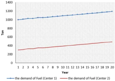
≤ + ∀ FFF T IBF T S F T, B B F T , , , , (21) Fig. 3. The demand for fuel.

(7)

∑

∑ ∑

+ ≤ × ∀ = − IBF T S M Y F T, B B F T t T K F K T , , , 0 1 , , (22) As previously mentioned, fuel blending plants can produce diﬀerent biodiesel blends. For this purpose, this study considers ﬁve fuels,

namely B5, B10, B20, B40, and B100. The maximum possible quantity of produced fuels, with received biodiesel in fuel blending plant, is presented by the following equations. Based on this equation, the sum of biodiesel used for producing diﬀerent biodiesel blends in a blending plant should be lower than the available biodiesel in that blending Fig. 5. The capacity of produced fuels in (Z1 = 6778417, Z2 = 16031586).

Fig. 6. Required agricultural farm area in (Z1 = 6778417, Z2 = 16031586).

(8)

plant. × + × + × + × + ≤ ∀ PF PF PF PF P F FF F T 0.05 0.1 0.2 0.4 , B F T B F T B F T B F T B F T F T 5, , 10, , 20, , 40, , 100, , , (23)

It is assumed that at any time and in any fuel blending plants, only one of biodiesel blends can be produced at the same time; Eqs.(24) and (25)explain this concept.

≤ × ∀ PFK F T, , M VK F T, , K T F, , (24)

∑

V ≤1 ∀T F, K K F T, , (25) Eqs.(27) to (31)calculate the quantity of consumed diesel to pro-duce each biodiesel blend. Eq.(27)conveys that for producing one liter B5, there is a need for 0.95 L diesel. Eqs. (28)–(30) explain similar concepts for B10, B20, and B40. Moreover, Eq.(31)calculates the total diesel which is needed for producing these blends.

≥ × = ∀ GOSK F T, , 0.95 PFK F T, , K B5, T F, (27) ≥ × = ∀ GOSK F T, , 0.9 PFK F T, , K B10, T F, (28) ≥ × = ∀ GOSK F T, , 0.8 PFK F T, , K B20, T F, (29) ≥ × = ∀ GOSK F T, , 0.6 PFK F T, , K B40, T F, (30)

∑

≥ ∀ SDF T GOS T F, K K F T , , , (31) Actually, according to the mentioned equations, the cost of biodiesel blends is calculated by the concept in the following equation.

= ×

+ ×

Biodiesel Blend Cost

Biodiesel blends share Biodiesel Cost Diesel share Diesel Cost

_ _

[( _ _ _ )

( _ _ )] (32)

The relationship between the produced and the transported bio-diesel blends to demand centers presented in Eq.(33). This equation conveys that the amount of fuel type K that is produced in a blending plant should be higher than the sum of fuel that is sent from that plant to different demand centers. Furthermore, Eq.(34) shows the ful fill-ment of demands by biodiesel fuels and diesel. Based on this equation, the demand in a center should be fulfilled by different biodiesel blends that are sent to that center from different blending plants and con-ventional diesel.

∑

≥ ∀ PFK F T S F K T, , C F K C T , , , , , (33)

∑ ∑

+ ≥ ∀ GDC T S D C T, F K F K C T C T , , , , , (34) In the following, similar concepts have been presented for the produced glycerin in the process. The produced glycerin in each bio-diesel reﬁnery is calculated by Eq.(35).

≤ × ∀

PGLB T, αgli FBB T, B T, (35)

Eqs.(36)–(39)show relationships among the produced glycerin, the imported glycerin and the transported glycerin from each biodiesel reﬁnery to demand center.

∑

≥ ∀ PGLB T S B T, GL B GL T , , , (36)

∑

≤ ∀ FGLGL T S GL T, B B GL T , , , (37)

∑

≥ ∀ FGLGL T S GL T, GLD GL GLD T , , , (38)

∑

S +IGL ≥D ∀ T GLD, GL GL GLD T, , GLD T, GLD T, (39) The capacities of facilities have been presented in Eqs.(40)–(51). The refined waste oil, oil, biodiesel, glycerin, and fuel must be pro-portional to the available capacities of related facilities. Eqs.(40) and (41)are about produced oil and the capacity of oil extraction plants. Eqs.(42) and (43)show the relationships between produced biodiesel and the capacity of the biodiesel refineries. Eqs.(44) and (45)consider relationships between produced glycerin and the capacity of the bio-diesel refineries. Eqs.(46) and (47)are about refined waste oil and the capacity of the waste oil refineries. The flow of glycerin to demand centers and the capacity of glycerin distributor are presented by Eqs. (48) and (49). The relationships between biodiesel blends and the fuel blending plants are calculated by Eqs.(50) and (51).

∑

≤ ∀ POO T CO O T, T O T , , (40) ≤ × ∀ COO T, M YO T, O T, (41)

∑

≤ ∀ PBB T CB B T, T B T , , (42) ≤ × ∀ CBB T, M YB T, B T, (43)

∑

≤ ∀ PGLB T CB B T, T B Gli T , , , (44) ≤ × ∀ CBB Gli T, , M YB T, B T, (45)

(9)

∑

≤ ∀ PRWW T CW W T, T W T , , (46) ≤ × ∀ CWW T, M YW T, W T, (47)

∑

S ≤

∑

CGL ∀GL T, B B GL T T GL T , , , (48) ≤ × ∀ CGLGL T, M YGL T, GL T, (49)

∑

≤

∑

∀ = PF CF F T, K K F T t T F T , , 0 , (50) ≤ × ∀ CFF T, M YF T, F T, (51) Numerical example

In this section, an example based on a real case study has been created and solved using an augmentedε-constraint method that it is explained by Mavrotas and Florios [35]. This method improves the conventional ε-constraint method for generating the Pareto optimal solutions. This method addresses some weak points of the conventional ε-constraint, namely, the guarantee of Pareto optimality of the obtained solution in the payoﬀ table as well as in the generation process and the increased solution time for problems with several objective functions.

In the conventional ε-constraint method, one of the objective functions is optimized using the other objective functions as constraints, incorporating them in the constraint part of the model. In this method by parametrical variation in the RHS (e1, e2,…, ep) of the constrained

objective functions, the eﬃcient solutions of the problem are obtained [36]. But this method may produce weakly Pareto optimal solutions. The augmentedε-constraint method is a method that tries to avoid this problem and accelerate the whole process. The new model for the augmentedε-constraint method becomes:

In this model, S2,… , Spare the surplus variables of the constraints

andε is an adequately small number between 10-6and 10-3[36]. In this study, this method has been implemented in the GAMS environment using CPLEX solver.Table 2shows the considered value for the indexes andTable 3shows the value of the parameters (Table 4).

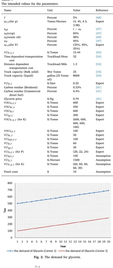
The input in this study is gathered with the help of experts in Renewable Energy and Energy Eﬃciency Organization (SATBA)[37] and Niroo Research Institute (NRI)[38].Figs. 2 and 3show the con-sidered demands of fuel and glycerin in demand centers. It is assumed that the demands are increasing with steady gradients.

Furthermore, to calculate second objective function, there is some study that considered the emission of biodiesel and their blends [39,40]. This study uses the information of a study by Budzaky et al. [41].

Results and discussion

This section presents the model implementation results for this ex-ample.Fig. 4shows an exact Pareto set which consists of ten points. In theε-constraint method, diﬀerent values were examined and ﬁnally, the value of 10-3_{was chosen for}_{ε since it led to the biggest penalty and}

better results. Each of these points is an exact solution for the model, and decision-makers can select their own desired point among them. As can be seen, the eﬀorts to reduce the value of the second objective lead to exponential growth in cost objective.

As an example, one of the solutions, namely (Z1= 6778417,

Z2= 16031586), and its results are described in the following.Fig. 5

presents the cumulative capacity of produced diesel blends. In this so-lution, B5 is produced in region 2, and B40 is produced in region 1 and region 3.

Among the crops and waste oil, the second crop, namely sunﬂower is the best resource for oil producing.Fig. 6shows the required farm’s area in each region. Moreover,Fig. 7presents the capacity of the oil extraction plant in each location.

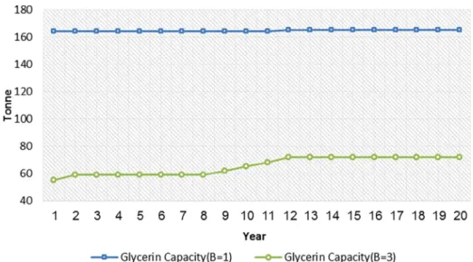
Fig. 8shows the capacities of glycerin production facilities during the optimization period.

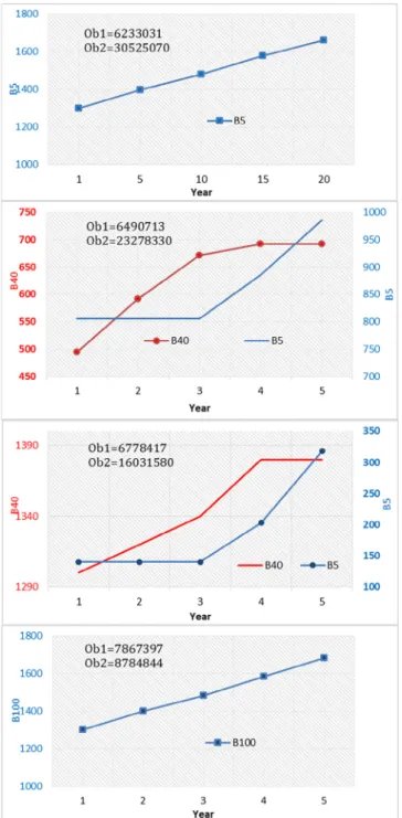
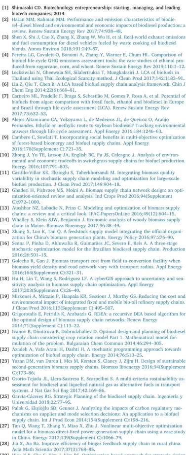
Furthermore,Fig. 9indicates the optimum blends of fuels for four solutions in the exact Pareto set.

According to the results, a decrease in the second objective (en-vironmental eﬀects objective) leads to a higher proportion of biodiesel in the produced fuels. When (Z1 = 6233031, Z2 = 30525070) the fuel is B5. In (Z1 = 6490713, Z2 = 23278330) B40 and B5 are the best fuels, and in (Z1 = 6778417, Z2 = 16031580) B40, and B5 are se-lected. However, the share of B40 is more than (Z1 = 6490713, Z2 = 23278330) in this solution. Moreover, in (Z1 = 7867397, Fig. 9. The best biodiesel blends for four solutions of pareto set.

(10)

Z2 = 8784844), B100 is considered as the best fuel according to con-ditions by the model. As it is seen inFig. 9andTable 7, B5 and B40 are the best biodiesel blends which are reasonable in the majority points of the Pareto set; consequently, these fuels should be considered for the gradual development of the biodiesels.

Table 5shows the value of the decision variables. The capacity of the waste oil refinery in all solutions, except the fourth solution, is approximately zero. In other words, based on the input data, in the production of biodiesel, using crops is more economical than using waste oil; the used diesel to fulfill the considered demands is also ap-proximately zero. Therefore, biodiesel blends fulfill most of the

demands. As mentioned before, a decrease in environmental effects causes an increase in costs. Furthermore, this decrease leads to a higher proportion of biodiesel in biodiesel blends. Thus, the capacities of fa-cilities, namely oil plant, glycerin plant, and biodiesel refinery, etc. are increased. In the fourth solution, the dimension of the farm is de-creased, and the capacity of the waste oil refinery is more than other solutions.

Sensitivity analysis

This section surveys the sensitivity analysis of the results. For this Table 5

The value of diﬀerent variables for four solutions of Pareto set in the base model.

No. Objectives Variables Year

1 5 10 15 20

1 Z1 = 6233031

Z2 = 30525070

Farm usage (Cumulative) (Hectare) 20 21 22 23 24

Capacity of oil plant (Cumulative) (Tonne) 78 84 89 95 97

Capacity of Glycerin (Cumulative) (Tonne) 27 29 30.5 33 33.5

Capacity of Waste oil reﬁnery (Cumulative) (Tonne) 0 0 0 0 1.3

Capacity of Glycerin supplier (Cumulative) (Tonne) 23 23 23 23 23 Capacity of Biodiesel reﬁnery (Cumulative) (Tonne) 65 70 74 79 82

Used Diesel at Demand Center (Tonne/Year) 0 0 0 0 19.5

Imported Biodiesel (Tonne/Year) 0 0 0 0 0

2 Z1 = 6490713

Z2 = 23278330

Capacity of Glycerin (Cumulative) (Tonne) 100 117 130 135 136

Capacity of Waste oil reﬁnery (Cumulative) (Tonne) 0 0 0 0 0

Capacity of Glycerin supplier (Cumulative) (Tonne) 100 116 116 116 116 Capacity of Biodiesel reﬁnery (Cumulative) (Tonne) 238 277 309 321 323

Used Diesel at Demand Center (Tonne/Year) 0 0 0 0 0

3 Z1 = 6778417

Z2 = 16031580

Capacity of oil plant (Cumulative) (Ton) 626 636 654 666 666

Capacity of Glycerin (Cumulative) (Ton) 219 222 228 235 235

Capacity of Waste oil reﬁnery (Cumulative) (Ton) 0 0 0 0 5

Capacity of Glycerin supplier (Cumulative) (Ton) 164 164 164 164 164 Capacity of Biodiesel reﬁnery (Cumulative) (Tonne) 520 528 543 561 561

4 Z1 = 7867397

Z2 = 8784844

Capacity of Glycerin (Cumulative) (Tonne) 548 589 624 668 676

Capacity of Waste oil reﬁnery (Cumulative) (Tonne) 628 746 844 1036 1036 Capacity of Glycerin supplier (Cumulative) (Tonne) 426 442 442 442 442 Capacity of Biodiesel reﬁnery (Cumulative) (Tonne) 1300 1398 1480 1580 1640

(11)

Fig. 11. The value of objectives in exact pareto set for 20% decrease in diesel price.

Fig. 12. The value of objectives in exact pareto set for 20% increase in diesel price.

Table 6

The value of the objective functions for the base model and three sensitivity analyses.

Base Interest rate (10%) Diesel price (−20%) Diesel price (+20%)

First Solution Z1 = 6233031 Z1 = 4414921 Z1 = 5370001 Z1 = 14390780 Z2 = 30525070 Z2 = 30525070 Z2 = 30525010 Z2 = 6841668 Second Solution Z1 = 6316395 Z1 = 4476965 Z1 = 5487716 Z1 = 14792750 Z2 = 28109490 Z2 = 28109470 Z2 = 28109430 Z2 = 6794427 Third Solution Z1 = 6403566 Z1 = 4564246 Z1 = 5622534 Z1 = 15214450 Z2 = 25693910 Z2 = 25693890 Z2 = 25693860 Z2 = 6747187 Fourth Solution Z1 = 6490713 Z1 = 4653036 Z1 = 5758570 Z1 = 15674870 Z2 = 23278330 Z2 = 23278330 Z2 = 23278290 Z2 = 6699946 Fifth Solution Z1 = 6577613 Z1 = 4742181 Z1 = 5894627 Z1 = 16197250 Z2 = 20862750 Z2 = 20862740 Z2 = 20862710 Z2 = 6652706 Sixth Solution Z1 = 6664502 Z1 = 4831490 Z1 = 6030116 Z1 = 16770480 Z2 = 18447170 Z2 = 18447160 Z2 = 18447140 Z2 = 6605466 Seventh Solution Z1 = 6778417 Z1 = 4920858 Z1 = 6166085 Z1 = 17416950 Z2 = 16031580 Z2 = 16031580 Z2 = 16031560 Z2 = 6558225 Eighth Solution Z1 = 6856997 Z1 = 5023027 Z1 = 6333143 Z1 = 18173990 Z2 = 13616000 Z2 = 13616000 Z2 = 13615990 Z2 = 6510985 Ninth solution Z1 = 7038972 Z1 = 5313880 Z1 = 6806396 Z1 = 19049670 Z2 = 11200420 Z2 = 11200420 Z2 = 11200410 Z2 = 6463744 Tenth Solution Z1 = 7867397 Z1 = 5874861 Z1 = 7821783 Z1 = 19936240 Z2 = 8784844 Z2 = 8784844 Z2 = 8784838 Z2 = 6416504

(12)

purpose, the eﬀects of changes in the interest rate and diesel price are considered.Fig. 10shows the sensitivity analysis of the results for the interest rate. Results show that an increase in the interest rate to 10% causes a decrease in theﬁrst objective in comparison to 5% interest rate.

Figs. 11 and 12 show the sensitivity analysis of exact Pareto set concerning diesel price.

Table 6shows a summary of these exact Pareto sets.

Table 7presents the produced biodiesel fuels for each of the solu-tions.

Based on the results of the sensitivity analysis, a decrease in the diesel price and an increase in the interest rate, do not cause any change in the combination of produced fuels; however, a 20% increase in diesel price leads to the production of B100.

Conclusion

In this paper, a comprehensive study is carried out with the aim of biodiesel development using a multi-objective and multi-period MIP model. The objectives of the model are the minimization of costs and environmental effects, and the study uses an augmented e-constraint method to get the exact Pareto set. The main aims of this study are to select the best primary resources among waste oil and different crops as well as the best fuels among B5, B10, B20, B40, B100, and diesel to fulfill fuel demands during an optimization period. The model selects the best fuels and the capacities of facilities according to the conditions. The results show that the objectives are in conflict with each other and a reduction in environmental effects leads to an increase in costs. Furthermore, it causes the use of a higher biodiesel proportion in the produced fuels. For example, in the best value for environmental ef-fects, B100 is selected, but in the worst value, B5 is considered as the best fuel. Moreover, at the midpoints of exact Pareto set, the combi-nation of several biodiesel blends are selected; for instance, in the point of (Z1 = 6778417, Z2 = 16031580) B40 and B5 are selected as the best fuels by the model. All in all, the results demonstrate that B5 and B40 are the best biodiesel blends that are reasonable in most of the points. Consequently, these fuels should be considered for the gradual devel-opment of the biodiesels.

The biodiesel is more expensive than conventional fuels like fossil fuels in most countries; therefore, replacing conventional fuels with biodiesel blends is diﬃcult. However, fuels with a higher biodiesel proportion release less pollution. On the other hand, due to climate change and global warming and its international commitments, a gra-dual tendency towards cleaner fuels seems a rational decision. Based on the obtained results through this study, the presented model can help decision-makers for designing a development plan considering the fu-ture requirements and restrictions.

Appendix A. Supplementary data

Supplementary data to this article can be found online athttps:// doi.org/10.1016/j.seta.2019.100545.

References

[1] Shimasaki CD. Biotechnology entrepreneurship: starting, managing, and leading biotech companies; 2014.

[2] Hasan MM, Rahman MM. Performance and emission characteristics of biodie-sel–diesel blend and environmental and economic impacts of biodiesel production: a review. Renew Sustain Energy Rev 2017;74:938–48.

[3] Shen X, Shi J, Cao X, Zhang X, Zhang W, Wu H, et al. Real-world exhaust emissions and fuel consumption for diesel vehicles fueled by waste cooking oil biodiesel blends. Atmos Environ 2018;191:249–57.

[4] Pereira LG, Cavalett O, Bonomi A, Zhang Y, Warner E, Chum HL. Comparison of biofuel life-cycle GHG emissions assessment tools: the case studies of ethanol pro-duced from sugarcane, corn, and wheat. Renew Sustain Energy Rev 2019;110:1–12. [5] Lecksiwilai N, Gheewala SH, Silalertruksa T, Mungkalasiri J. LCA of biofuels in

Thailand using Thai Ecological Scarcity method. J Clean Prod 2017;142:1183–91. [6] Liu Z, Qiu T, Chen B. A LCA based biofuel supply chain analysis framework. Chin J

Chem Eng 2014;22(6):669–81.

[7] Carneiro ML, Pradelle F, Braga S, Sebastião M, Gomes P, Rosa A, et al. Potential of biofuels from algae: comparison with fossil fuels, ethanol and biodiesel in Europe and Brazil through life cycle assessment (LCA). Renew Sustain Energy Rev 2017;73:632–53.

[8] Alejos Altamirano CA, Yokoyama L, de Medeiros JL, de Queiroz O, Araújo Fernandes. Ethylic or methylic route to soybean biodiesel? Tracking environmental answers through life cycle assessment. Appl Energy 2016;184:1246–63. [9] Cambero C, Sowlati T. Incorporating social beneﬁts in multi-objective optimization

of forest-based bioenergy and biofuel supply chains. Appl Energy 2016;178(Supplement C):721–35.

[10] Zhong J, Yu TE, Larson JA, English BC, Fu JS, Calcagno J. Analysis of environ-mental and economic tradeoﬀs in switchgrass supply chains for biofuel production. Energy 2016;107:791–803.

[11] Castillo-Villar KK, Eksioglu S, Taherkhorsandi M. Integrating biomass quality variability in stochastic supply chain modeling and optimization for large-scale biofuel production. J Clean Prod 2017;149:904–18.

[12] Ghaderi H, Pishvaee MS, Moini A. Biomass supply chain network design: an opti-mization-oriented review and analysis. Ind Crops Prod 2016;94(Supplement C):972–1000.

[13] Atashbar NZ, Labadie N, Prins C. Modeling and optimization of biomass supply chains: a review and a critical look. IFAC-PapersOnLine 2016;49(12):604–15. [14] Whalley S, Klein SJW, Benjamin J. Economic analysis of woody biomass supply

chain in Maine. Biomass Bioenergy 2017;96:38–49.

[15] Zhang X, Luo K, Tan Q. A feedstock supply model integrating the oﬃcial organi-zation for China's biomass generation plants. Energy Policy 2016;97:276–90. [16] Senna P, Pinha D, Ahluwalia R, Guimarães JC, Severo E, Reis A. A three-stage

stochastic optimization model for the Brazilian biodiesel supply chain. Production 2016;26:501–15.

[17] Golecha R, Gan J. Biomass transport cost fromﬁeld to conversion facility when biomass yield density and road network vary with transport radius. Appl Energy 2016;164(Supplement C):321–31.

[18] Hu H, Lin T, Wang S, Rodriguez LF. A cyberGIS approach to uncertainty and sen-sitivity analysis in biomass supply chain optimization. Appl Energy

2017;203(Supplement C):26–40.

[19] Mirkouei A, Mirzaie P, Haapala KR, Sessions J, Murthy GS. Reducing the cost and environmental impact of integratedﬁxed and mobile bio-oil reﬁnery supply chains. J Clean Prod 2016;113(Supplement C):495–507.

[20] Grigoroudis E, Petridis K, Arabatzis G. RDEA: a recursive DEA based algorithm for the optimal design of biomass supply chain networks. Renew Energy

2014;71(Supplement C):113–22.

[21] Ivanov B, Dimitrova B, Dobrudzhaliev D. Optimal design and planning of biodiesel supply chain considering crop rotation model Part 1. Mathematical model for-mulation of the problem. Bulgaraian Chem Commun 2014;46:294–305. [22] Azadeh A, Vafa Arani H, Dashti H. A stochastic programming approach towards

optimization of biofuel supply chain. Energy 2014;76:513–25.

[23] Yazan DM, van Duren I, Mes M, Kersten S, Clancy J, Zijm H. Design of sustainable second-generation biomass supply chains. Biomass Bioenergy 2016;94(Supplement C):173–86.

[24] Osorio-Tejada JL, Llera-Sastresa E, Scarpellini S. A multi-criteria sustainability as-sessment for biodiesel and liqueﬁed natural gas as alternative fuels in transport systems. J Nat Gas Sci Eng 2017;42:169–86.

[25] García-Cáceres RG. Strategic Planning of the biodiesel supply chain. Ingeniería y Universidad 2018;22:77–95.

[26] Palak G, Ekşioğlu SD, Geunes J. Analyzing the impacts of carbon regulatory me-chanisms on supplier and mode selection decisions: An application to a biofuel supply chain. Int J Prod Econ 2014;154(Supplement C):198–216.

[27] Tan Q, Wang T, Zhang Y, Miao X, Zhu J. Nonlinear multi-objective optimization model for a biomass direct-ﬁred power generation supply chain using a case study in China. Energy 2017;139(Supplement C):1066–79.

[28] Jia X, Jia Ra. Improve eﬃciency of biogas feedback supply chain in rural china. Acta Math Scientia 2017;37(3):768–85.

[29] Woo Y-B, Cho S, Kim J, Kim BS. Optimization-based approach for strategic design

Table 7

The best biodiesel blends for the base model and three sensitivity analyses. Base Interest rate

(10%) Diesel price (−20%) Diesel price (+20%) First Solution B5 B5 B5 B100 Second Solution B5, B40 B5, B40 B5, B40 B100 Third Solution B5, B40 B5, B40 B5, B20, B40 B100 Fourth Solution B5, B40 B5, B40 B5, B40 B100 Fifth Solution B5, B40 B5, B40 B5, B40 B100 Sixth Solution B5, B40 B5, B40 B5, B40 B100 Seventh Solution B5, B40 B5, B40 B5, B40 B100 Eighth Solution B40, B100 B40, B100 B40, B100 B100 Ninth solution B40, B100 B40, B100 B40, B100 B100 Tenth Solution B100 B100 B100 B100

(13)

and operation of a biomass-to-hydrogen supply chain. Int J Hydrogen Energy 2016;41(12):5405–18.

[30] Guillén-Gosálbez G, Mele FD, Grossmann IE. A bi-criterion optimization approach for the design and planning of hydrogen supply chains for vehicle use. AIChE J 2010;56(3):650–67.

[31] Jeong H, Sieverding H, Stone J. Biodiesel supply chain optimization modeled with geographical information system (GIS) and mixed-integer linear programming (MILP) for the Northern Great Plains Region. Bioenergy Res 2018;12:1–5. [32] De Laporte AV, Weersink AJ, McKenney DW. Eﬀects of supply chain structure and

biomass prices on bioenergy feedstock supply. Appl Energy 2016;183(Supplement C):1053–64.

[33] Lainez-Aguirre JM, Pérez-Fortes M, Puigjaner L. Economic evaluation of bio-based supply chains with CO2 capture and utilisation. Comput Chem Eng

2017;102(Supplement C):213–25.

[34] Fukuda H, Kondo A, Noda H. Biodiesel fuel production by transesteriﬁcation of oils. J Biosci Bioeng 2001;92(5):405–16.

[35] Mavrotas G, Florios K. An improved version of the augmentedε-constraint method (AUGMECON2) forﬁnding the exact pareto set in multi-objective integer pro-gramming problems. Appl Math Comput 2013;219(18):9652–69.

[36] Mavrotas G. Eﬀective implementation of the ε-constraint method in Multi-Objective Mathematical Programming problems. Appl Math Comput 2009;213(2):455–65. [37] Organization, R.E.a.E.E., 2019. Available from:http://www.satba.gov.ir/en/home. [38] Institute, N.R.

[39] Azad K, Rasul M, Giannangelo B, Islam R. Comparative study of diesel engine performance and emission with soybean and waste oil biodiesel fuels. Int J Autom Mech Eng 2016;12:2866–81.

[40] Lahane S, Subramanian KA. Eﬀect of diﬀerent percentages of biodiesel–diesel blends on injection, spray, combustion, performance, and emission characteristics of a diesel engine. Fuel 2015;139:537–45.

[41] Budžaki S, Miljić G, Tišma M, Sundaram S, Hessel V. Is there a future for enzymatic biodiesel industrial production in microreactors? Appl Energy

2017;201(Supplement C):124–34.

[42] Silva Filho SCd, et al. Environmental and techno-economic considerations on bio-diesel production from waste frying oil in São Paulo city. J Clean Prod 2018;183:1034–42.

[43] Sakdasri W, Sawangkeaw R, Ngamprasertsith S. Techno-economic analysis of bio-diesel production from palm oil with supercritical methanol at a low molar ratio. Energy 2018;152:144–53.

[44] Ezzati F, Babazadeh R, Donyavi A. Optimization of multimodal, multi-period and complex biodiesel supply chain systems: case study. Renew Energy Focus 2018;26:81–92.

[45] Tran NN, et al. Scale-up and economic analysis of biodiesel production from re-cycled grease trap waste. Appl Energy 2018;229:142–50.

[46] Osmani A, Zhang J. Multi-period stochastic optimization of a sustainable multi-feedstock second generation bioethanol supply chain− a logistic case study in Midwestern United States. Land Use Policy 2017;61(Supplement C):420–50. [47] Babazadeh R, et al. An integrated data envelopment analysis–mathematical

pro-gramming approach to strategic biodiesel supply chain network design problem. J Clean Prod 2017;147(Supplement C):694–707.

[48] Babazadeh R. Optimal design and planning of biodiesel supply chain considering non-edible feedstock. Renew Sustain Energy Rev 2017;75:1089–100.

[49] Jensen IG, Münster M, Pisinger D. Optimizing the supply chain of biomass and biogas for a single plant considering mass and energy losses. Eur J Oper Res 2017;262(2):744–58.

[50] Özdenkçi K, et al. A novel bioreﬁnery integration concept for lignocellulosic bio-mass. Energy Convers Manage 2017;149(Supplement C):974–87.

[51] Tan Q, et al. Nonlinear multi-objective optimization model for a biomass direct-ﬁred power generation supply chain using a case study in China. Energy 2017;139(Supplement C):1066–79.

[52] Madiwale S, Bhojwani V. An overview on production, properties, performance and emission analysis of blends of biodiesel. Procedia Technol 2016;25:963–73. [53] Mohseni S, Pishvaee MS. A robust programming approach towards design and

optimization of microalgae-based biofuel supply chain. Comput Ind Eng 2016;100(Supplement C):58–71.

[54] Azadeh A, Vafa Arani H. Biodiesel supply chain optimization via a hybrid system dynamics-mathematical programming approach. Renew Energy

2016;93(Supplement C):383–403.

[55] Zhang F, et al. Decision support system integrating GIS with simulation and opti-misation for a biofuel supply chain. Renew Energy 2016;85:740–8.

[56] Mohseni S, Pishvaee MS, Sahebi H. Robust design and planning of microalgae biomass-to-biodiesel supply chain: a case study in Iran. Energy

2016;111(Supplement C):736–55.

[57] Hombach LE, et al. Optimal design of supply chains for second generation biofuels incorporating European biofuel regulations. J Clean Prod 2016;133(Supplement C):565–75.

[58] Shabani N, Sowlati T. A hybrid multi-stage stochastic programming-robust opti-mization model for maximizing the supply chain of a forest-based biomass power plant considering uncertainties. J Clean Prod 2016;112(Part 4):3285–93. [59] Miret C, et al. Design of bioethanol green supply chain: Comparison betweenﬁrst

and second generation biomass concerning economic, environmental and social criteria. Comput Chem Eng 2016;85(Supplement C):16–35.

[60] Ivanov B, Stoyanov S. A mathematical model formulation for the design of an in-tegrated biodiesel-petroleum diesel blends system. Energy 2016;99:221–36. [61] Rincón LE, et al. Optimization of the Colombian biodiesel supply chain from oil

palm crop based on techno-economical and environmental criteria. Energy Econ 2015;47(Supplement C):154–67.

[62] Sakthivel G, Ilangkumaran M, Gaikwad A. A hybrid multi-criteria decision mod-eling approach for the best biodiesel blend selection based on ANP-TOPSIS analysis. Ain Shams Eng J 2015;6(1):239–56.

[63] Ahn Y-C, et al. Strategic planning design of microalgae biomass-to-biodiesel supply chain network: Multi-period deterministic model. Appl Energy

2015;154(Supplement C):528–42.

[64] Paulo H, et al. Supply chain optimization of residual forestry biomass for bioenergy production: the case study of Portugal. Biomass Bioenergy 2015;83(Supplement C):245–56.

[65] Sharifzadeh M, Garcia MC, Shah N. Supply chain network design and operation: systematic decision-making for centralized, distributed, and mobile biofuel pro-duction using mixed integer linear programming (MILP) under uncertainty. Biomass Bioenergy 2015;81:401–14.

[66] Liu Z, Qiu T, Chen B. A study of the LCA based biofuel supply chain multi-objective optimization model with multi-conversion paths in China. Appl Energy 2014;126(Supplement C):221–34.

[67] Aldana H, Lozano FJ, Acevedo J. Evaluating the potential for producing energy from agricultural residues in México using MILP optimization. Biomass Bioenergy 2014;67(Supplement C):372–89.

[68] Blake LI, et al. Evaluating an anaerobic digestion (AD) feedstock derived from a novel non-source segregated municipal solid waste (MSW) product. Waste Manage 2017;59:149–59.

[69] Zhang Y, Jiang Y. Robust optimization on sustainable biodiesel supply chain pro-duced from waste cooking oil under price uncertainty. Waste Manage 2017;60(Supplement C):329–39.