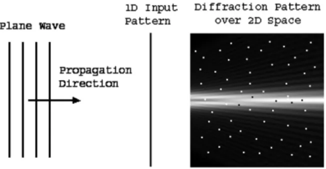
Diffraction field computation from arbitrarily distributed data points in space

Discussion of the following terms: onscreen space, offscreen space, open space and closed space?. (pages 184-191 from the book Looking

Hematopia: Lung hemorrhage, oral bleeding Hematomesis: Stomach bleeding, oral bleeding Melena: Gastrointestinal bleeding, blood in the stool. Hematuria: Blood in urine, bloody

OKB yaygýnlýðý kadýnlarda %7.1 ve erkeklerde %5.3 olarak bulunurken, babanýn eðitim düzeyi, ailede ruhsal hastalýk hikayesi ve sigara kullanýmý ile OKB varlýðý arasýnda

Variety of different people /cultures Areas for young and adults Flexible spaces for Various uses Forms and Using quality Easier, Comfortable Use Long-lived designs Flexibility

well connected nodes and connecting paths and less saturated, cooler and darker color values to less connected, second and third order nodes and paths is a viable usage of using

yfihutta(idarei hususiyelerin teadül cetveli) gibi ömrümde bir defa bir yaprağına göz atmiyacağua ciltlerden başliyarak bütün bir kısmından ayrılmak zarurî,

John Krystal, depresyon durumunda olan kişilerin dış dünyadaki kontrastı daha az algılayabildiklerini, bu nedenle de dünyanın daha az eğlenceli bir yer olarak

Keywords: waterfront, coastline, critical delineation, critique of urbanization, material flows, material unfixity, urban edge, project, planetary space, port