Atmospheric Turbulence Modeling and Aperture Analysis
for Optimizing Receiver Design and System Performance
on Free Space Optical Communication Links
a thesis
submitted to the department of electrical and
electronics engineering
and the graduate school of engineering and sciences
of bilkent university
in partial fulfillment of the requirements
for the degree of
master of science
By
Hasim Meric
September 2012
I certify that I have read this thesis and that in my opinion it is fully adequate, in scope and in quality, as a thesis for the degree of Master of Science.
Prof. Dr. Ayhan Altınta¸s(Supervisor)
I certify that I have read this thesis and that in my opinion it is fully adequate, in scope and in quality, as a thesis for the degree of Master of Science.
Assist. Prof. Dr. Heba Y¨uksel(Co-supervisor)
I certify that I have read this thesis and that in my opinion it is fully adequate, in scope and in quality, as a thesis for the degree of Master of Science.
Assoc. Prof. Dr. Vakur B. Ert¨urk
I certify that I have read this thesis and that in my opinion it is fully adequate, in scope and in quality, as a thesis for the degree of Master of Science.
Assist. Prof. Dr. ¨Omer ˙Ilday
Approved for the Graduate School of Engineering and Sciences:
Prof. Dr. Levent Onural
ABSTRACT
Atmospheric Turbulence Modeling and Aperture Analysis
for Optimizing Receiver Design and System Performance
on Free Space Optical Communication Links
Hasim Meric
M.S. in Electrical and Electronics Engineering
Supervisor:
Prof. Dr. Ayhan Altınta¸s
and Assist. Prof. Dr. Heba Y¨
uksel
September 2012
Strong turbulence measurements that are taken using real time optical wireless experimental setups are valuable when studying the effects of turbulence regimes on a propagating optical beam. In any kind of Free Space Optical (FSO) system, knowing the strength of the turbulence thus the refractive index structure con-stant (Cn2), is beneficial for having an optimum bandwidth of communication. Even if the FSO Link is placed very well-high-above the ground just to have weak enough turbulence effects, there can be severe atmospheric conditions that can change the turbulence regime. Having a successful theory that will cover all regimes will give us the chance of directly processing the image in existing or using an additional hardware thus deciding on the optimum bandwidth of the communication line at firsthand.In literature, simulation of beam propaga-tion through turbulent media has always been a tricky subject when it comes to moderate-to-strong turbulent regimes. Creating a well controlled turbulent envi-ronment is beneficial as a fast and a practical approach when it comes to testing the optical wireless communication systems in diverse atmospheric conditions.
For all of these purposes, strong turbulence data have been collected using an outdoor optical wireless setup placed about 85 centimeters above the ground with an acceptable declination and a path length of about 250 meters inducing strong turbulence to the propagating beam. Variety of turbulence strength estimation methods as well as frame image analysis techniques are then been applied to the experimental data in order to study the effects of different parameters on the result. Such strong turbulence data is compared with existing weak and in-termediate turbulence data. The Aperture Averaging (AA) Factor for different turbulence regimes as well as the inner and outer scales of atmospheric turbulence are also investigated. A new method for calculating the Aperture Averaging Fac-tor is demonstrated deducing spatial features at the receiver plane. Controlled turbulent media is created using multiple phase screens each having supervised random variations in its frequency and power while the propagated beam is cal-culated using Fresnel diffraction method. The effect of the turbulent media is added to the propagated beam using the modified Von Karman spectrum. Cre-ated scintillation screens are tested and compared with the experimental data which are gathered in different turbulence regimes within various atmospheric conditions. We believe that the general drawback of the beam propagation sim-ulation is the difference in terms of spatial distribution and sequential phase textures. To overcome these two challenges we calculate the Aperture Averaging Factors to create more realistic results. In this manner, it is possible to create more viable turbulent like scintillations thus the relationship between the turbu-lence strength and the simulated turbuturbu-lence parameters are distinctly available. Our simulation gives us an elusive insight on the real atmospheric turbulent me-dia. It improves our understanding on parameters that are involved in real time intensity fluctuations that occur in every optical wireless communication system. Keywords: Free Space Optical Communication (FSO), Optical Wireless Links, Refractive Index Structure Constant(C2
Strong Atmospheric Turbulence, Scintillation Index, Aperture Averaging, Point Averaged Aperture Averaging, Phase Screens.
¨
OZET
AC
¸ IK ALAN OPT˙IK KOM˙IN˙IKASYON L˙INKLER˙I S˙ISTEM
PERFORMANSI ˙IC
¸ ˙IN ATMOSFER˙IK T ¨
URB ¨
ULANS
MODELLEME VE OPT˙IMUM ALICI AC
¸ IKLIK ANAL˙IZ˙I
Hasim Meric
Elektrik ve Elektronik M¨
uhendisli˘
gi B¨
ol¨
um¨
u Y¨
uksek Lisans
Tez Y¨
oneticisi: Prof. Dr. Ayhan Altınta¸s
ve Prof. Assist. Prof. Dr. Heba Y¨
uksel
Eyl¨
ul 2012
Ger¸cek zamanlı optik telekom¨unikasyon linkleri kullanılarak alınan g¨u¸cl¨u t¨urb¨ulans ¨Ol¸c¨umleri atmosferde ilerleyen I¸sık huzmesi ¨uzerindeki atmosferik etkileri incelemek i¸cin ¸cok de˘gerlidir. Kullanılan herhangi bir a¸cık alan optik kom¨unikasyon linkinde kırılma indisi yapısal sabitini bilmek veya ke-stirmek ileti¸sim hattının optimum bant geni¸sli˘gi hakkında bilgi edinmek i¸cin pek de˘gerlidir. A¸cık alan kom¨unikasyon linkinin ¸cok y¨uksek noktalara konu¸slandırıldı˘gı durumlarda bile iki alı¸sveri¸s¸ci arasında beklenmedik t¨urb¨ulans etkileri g¨or¨ulebilmektedir. T¨um t¨urb¨ulans rejimlerini kapsayacak genel bir teorinin varlı˘gı alıcı tarafında e¸szamanlı sinyal i¸sleyerek veya ek bir donanım yardımı ile kom¨unikasyon linkinin optimum bant geni¸sli˘gini ilk elde belirlemede etkili olacaktır. Literat¨urde ı¸sık huzmesinin t¨urb¨ulans ortamında ilerlemesi ¨
ozellikle orta ve y¨uksek g¨u¸cteki t¨urb¨ulans medyaları i¸cin dikkat ¸cekici bir konu olmu¸stur. ˙Iyi kontrol edilmi¸s ve belirlenen g¨u¸cte t¨urb¨ulans etkimi¸s bir ı¸sık huzmesi sim¨ulasyonu yapmak a¸cık alan optik kom¨unikasyon linkleri i¸cin hızlı pratik ve i¸se yarar bir y¨ontem te¸skil etmektedir.
T¨um bu nedenlerden dolayı, g¨u¸cl¨u t¨urb¨ulans verisi yerden 85 cm y¨ukseklik ve de kabul edilebilir e˘gimi olan 250 m uzunlukta deneysel bir alanda kuru-lan a¸cık akuru-lan optik kom¨unikasyon kurulumundan yararlanılarak elde edilmi¸stir. T¨urb¨ulansa etkiyen ve tetikleyen parametreler hakkında bilgi sahibi olabilmek i¸cin ¸ce¸sitli t¨urb¨ulans g¨u¸c hesaplama ve kestirim metotlarının yanında e¸szamanlı ¸cer¸ceve g¨or¨unt¨u analiz metotları da geli¸stirilmi¸stir. Elde edilen veriler var olan zayıf ve orta g¨u¸cteki t¨urb¨ulans verileri ile kar¸sıla¸stırılmı¸stır. Farklı g¨u¸cteki t¨urb¨ulans verilerinin ortalama a¸cıklık fakt¨or¨un¨un yanında atmosferik g¨u¸c spek-trumunun i¸csel ve dı¸ssal skala de˘gerleri ara¸stırılmı¸stır. Ortalama a¸cıklık fakt¨or¨u hesaplanmak ¨uzere mekansal ¨ozellikleri kullanarak yeni bir metot sunulmu¸stur. G¨uc¨u kontrol edilebilir bir t¨urb¨ulans ortamı seri olarak ¨onceden ortalaması ve de varyansı karar verilmi¸s rastgele atanmı¸s frekans ve g¨u¸c de˘gerlerine sahip faz ekranları kullanılıp ı¸sık huzmesinin yayılımı a¸cısal frensel kırlım metodu kul-lanılarak olu¸sturulmu¸stur. T¨urb¨ulans ortamının etkisi modifiye edilmi¸s von Kar-man spektrumu kullanılarak yayılan ı¸sık huzmesine etkimi¸stir. Alıcıda Yaratılan ı¸sıldama faz ekranı ile farklı t¨urb¨ulans rejimlerinde ve farklı deney ortamlarında alınan deneysel verilerimizin sonu¸cları kar¸sıla¸stırılıp test edilmi¸stir. Kestirilmek-tedir ki literat¨urdeki atmosferik ı¸sık huzmesi yayılımındaki sonu¸clara engel te¸skil eden fakt¨orler sıralı atmosferik faz dokusu ve de y¨uzeysel da˘gılımıdır ı¸sık huzmesi da˘gılımıdır. Bu iki engelin ¨ustesinden gelebilmek i¸cin sim¨ulasyon ve deneysel sonu¸cların ortalama a¸cıklık fakt¨orleri hesaplanmı¸stır. Bu sayede ger¸ce˘ge daha yakın t¨urb¨ulans ı¸sıldamaları elde etmek m¨umk¨un olup farklı t¨urb¨ulans rejim-lerinde t¨urb¨ulansa etki eden parametreler belirgin hale gelmektedir. Sim¨ulasyon sonu¸clarımız bize t¨urb¨ulans do˘gası ve ortamı hakkında ele gelmez bir i¸cg¨or¨u ver-mektedir. Aynı zamanda ger¸cek zamanlı t¨um optik a¸cık alan kom¨unikasyon lin-klerinde temel problem olan g¨u¸c yo˘gunlu˘gu dalgalanmaları ¨uzerinde etkili olan parametreler ¨uzerindeki anlayı¸sımızı g¨u¸clendirmektedir.
Anahtar Kelimeler: A¸cık Alan Optik Kominikasyonu, Kablosuz Optik Linkleri, Kırlma indisi kalıpsal sabiti, G¨u¸c Yo˘gunlu˘gu Varyansı, Rytov Varyansı, G¨u¸cl¨u
Atmospheric Turbulence, I¸sıldama ˙Indisi, A¸cıklık Ortalaması, Nokta Ortalamalı A¸cıklık Ortalama, Faz Ekranı
ACKNOWLEDGMENTS
First of all, I would like to give my inexpressible gratitude to my main supervisor Assist. Prof. Heba Y¨uksel, who was the most inspiring and influential person during my graduate studies. She has provided me with a great research envi-ronment with her positiveness, friendly approach and endless support. It was a great honor and privilege for me to work with her. My deepest respects and thanks goes to Prof. Ayhan Altınta¸s for agreeing to serve as my supervisor at the end of my thesis work.
Also, I would like to thank Assoc. Prof. Vakur Ert¨urk and Asst. Prof. ¨Omer ˙Ilday for their service in my thesis committee.
Finally, I especially would like to thank my family for their unconditional love and support.
Contents
1 INTRODUCTION 1
1.1 Overview of Turbulence . . . 1
1.2 Classical Theory . . . 4
1.3 Aperture Averaging Theory . . . 7
2 Simulation Model 10 2.1 Refractive Index Structure Constant (Cn2) Evaluation . . . 10
2.2 Phase Screen Method . . . 14
2.2.1 Introduction . . . 14
2.2.2 Phase screen Methodology . . . 16
2.2.3 Results . . . 20
2.3 Image Acquisition and Tracking Algorithm . . . 24
2.4 Analysis of turbulence strength for free space optical communica-tion using Support Vector Machine (SVM) regression methods . . 28
2.4.2 Feature Extraction . . . 29
2.4.3 Region Covariance Method . . . 29
2.4.4 Discrete wavelet transform (DWT) . . . 30
2.4.5 Complex Wavelet Transform . . . 31
2.4.6 Support Vector Machine Classification . . . 31
2.4.7 SVM Regression . . . 32
2.4.8 Results and Conclusions . . . 41
3 Experimental Setup 42 3.1 Strong Turbulence Setup . . . 42
3.1.1 Odeon Experimental Setup at Bilkent University . . . 42
3.1.2 Strong Turbulence Experiment at the University of Maryland 49 3.2 Acquiring further weak & intermediate turbulence data using the University of Maryland Setup . . . 58
3.3 Analysis of the turbulence results in weak-to-strong turbulence regimes . . . 61
3.4 Proposed Methods for Estimating Cn2: . . . 64
3.4.1 Portable C2 n Measurement using an Incoherent Source: . . 64
3.4.2 Turbulence Strength Estimation with Tracking Algorithm of the Beam from the Angle of Arrival (AOA) Variance . . 66
4.1 Comparison of the strong turbulence data with theory . . . 69
4.2 The Andrews Asymptotic Analysis . . . 70
4.3 Churnside’s Asymptotic Analysis . . . 71
4.4 Effective Kolmogorov Spectrum and Scintillation Index . . . 72
4.5 Comparison of the experimental data to the theory . . . 74
4.6 Effects of the inner scale . . . 79
4.7 Optimizing Receiver Design through analysis of the Aperture Av-eraging curves . . . 81
4.8 Optimizing System Performance through SNR and BER analysis 82
List of Figures
1.1 Atmospheric Layers. Source:Larry C. Andrews,Laser Beam Prop-agation Through Random Media,pg:10 . . . 2
1.2 Typical atmospheric transmittance for 1 km horizontal path, 3 meters above the ground, no fog, no rain, no clouds. Source:Larry C. Andrews,Laser Beam Propagation Through Random Media,pg:13 4
1.3 The Cascade theory of turbulence where Lo denotes the outer
scale and lo is the inner scale. Source:Larry C. Andrews,Laser
Beam Propagation Through Random Media,pg:60 . . . 5
2.1 The Cn2 image where the refractive index fluctuations occurs . . . 13 2.2 Modified Von Karman Spectrum vs the Von Karman spectrum . . 16
2.3 Fast Fluctuation Effect of the Optical turbulence on a 100 meter slant path with a Cn2 = 10−16. . . 18 2.4 Lower Fluctuation Effect of the Optical turbulence on a 100 meter
slant path with a C2
n = 10−16. . . 19
2.5 Simulation Result of Optical turbulence screen on a 100 meter slant path with a C2
n = 10
2.6 Strong Turb.(C2
n = 10−10) and Intermediate Turb.(Cn2 = 10−13)
Images, Path:100 m. l0 = 5mm and L0 = 104. . . 21
2.7 Weak Turb. Image, ,Path:100 m. C2 n = 10
−15, l
0 = 5mm and
L0 = 104. . . 21
2.8 Simulated Aperture Averaging Results over 100 meters for various C2
n values . . . 22
2.9 Experimental and Simulated Results of the Point Averaged Aper-ture Averaging Factor for C2
n= 2x10
−12, path length =120 meters,
l0 = 5mm and L0 = 104. . . 23
2.10 Experimental and Simulated Results of the Point Averaged Aper-ture Averaging Factor for C2
n= 5x10
−14, path length =120 meters,
l0 = 5mm and L0 = 104. . . 23
2.11 Intensity Distribution of the Image at the Receiver Side with no Turbulence Effects. . . 24
2.12 The view of the light path in the optical design of the telescope . 24 2.13 Turbulence induced image and Region result of the software . . . 25
2.14 Turbulence induced problematic image and the Region that is causing problems . . . 26 2.15 Binary image without smoothing and Binary image after smoothing 26
2.16 SVM Regression using 1-Level Wavelet transform with biorthonal filter . . . 33 2.17 SVM Regression using 1-Level Wavelet transform with biorthonal
2.18 SVM Regression using 3-Level Wavelet transform with biorthonal filter . . . 34 2.19 SVM Regression using 3-Level Wavelet transform with biorthonal
filter . . . 34 2.20 SVM Regression using 1-Level Wavelet transform with doubechies
filter . . . 35
2.21 SVM Regression using 1-Level Wavelet transform with doubechies filter . . . 35
2.22 SVM Regression using 3-Level Wavelet transform with doubechies filter . . . 36 2.23 SVM Regression using 3-Level Wavelet transform with doubechies
filter . . . 36
2.24 SVM Regression using Region Covariance method with first order statistics . . . 36
2.25 SVM Regression using Region Covariance method with first order statistics . . . 37
2.26 SVM Regression using Region Covariance method with second order statistics . . . 37 2.27 SVM Regression using Region Covariance method with second
order statistics . . . 37
2.28 SVM Regression using 1-Level Complex Wavelet transform . . . 38 2.29 SVM Regression using 1-Level Complex Wavelet transform . . . 38
2.31 SVM Regression using 2-Level Complex Wavelet transform . . . 39
2.32 SVM Regression using 3-Level Complex Wavelet transform . . . 39
2.33 SVM Regression using 3-Level Complex Wavelet transform . . . 40
2.34 SVM Regression using 4-Level Complex Wavelet transform . . . 40
2.35 SVM Regression using 4-Level Complex Wavelet transform . . . 40
3.1 Aperture Averaging Factor For Intermediate turbulence conditions 43 3.2 Experimental Location . . . 44
3.3 Enclosed Transmitter and Transmitter part front-view . . . 45
3.4 Transmitter side with line-of-sight and Transmitter side (close view) 45 3.5 Receiver part - Front view and Receiver Part - Back view . . . 46
3.6 The receiver side showing line of sight. and Receiver side con-nected to CCD camera with an adapter . . . 47
3.7 Sample images from Bilkent University Strong Turbulence Setup. 47 3.8 AA factor for the Bilkent University Strong Turbulence Setup. . . 48
3.9 Overall Schematic of the experiment. . . 49
3.10 Line of Sight shown from the TX side. . . 50
3.11 Top view of the experiment. . . 50
3.12 Transmitter Side. . . 51
3.13 Receiver Side. . . 52
3.15 Histogram of Faulty images. . . 53
3.16 Histogram of Appropriate images. . . 54
3.17 Sample of a strong turbulence induced beam shape . . . 54
3.18 Aperture averaging factor for different center points on the beam. 55 3.19 Point Averaged Aperture Averaging Factor for strong turbulence data. . . 55
3.20 Illustration for Point Averaged Aperture Averaging . . . 56
3.21 Point Averaged Aperture Averaging Factor for strong turbulence data. . . 57
3.22 Weak-Intermediate Turbulence FSO Link. . . 58
3.23 Weak Turbulence Beam Shape Results. . . 59
3.24 Aperture Averaging Factor For weak turbulence data. . . 60
3.25 Combined Aperture Averaging Factors for different turbulence regimes. . . 61
3.26 Combined AA Curves for different turbulence regimes. . . 62
3.27 Bilkent University Strong Turbulence setup versus UMD Strong Turbulence Setup. . . 63
3.28 Portable C2 n Measurement Setup. . . 64
3.29 C2 n value in 100 meters- Hallway experiment with hotwave plate. . 65
3.30 Overall picture of the transmitter with the beam to track on the middle. . . 68
3.31 Result of the Beam tracking Algorithm. . . 68
4.1 Experimental Results and Theoretical Results of Aperture Averag-ing Factor for Cn2structure parameter of 2.31x10⁻¹⁵and Resulted
Error margin of 36%. . . 75 4.2 Experimental Results and Theoretical Results of Aperture
Averag-ing Factor for Cn2structure parameter of 1.77x10⁻¹⁴and Resulted
Error margin of 32%. . . 75 4.3 Experimental Results and Theoretical Results of Aperture
Averag-ing Factor for Cn2structure parameter of 1.73x10⁻¹⁴and Resulted
Error margin of 44.76%. . . 76 4.4 Experimental Results and Theoretical Results of Aperture
Averag-ing Factor for Cn2structure parameter of 1.98x10⁻¹⁴and Resulted
Error margin of 27.5%. . . 76 4.5 Experimental Results and Theoretical Results of Aperture
Averag-ing Factor for Cn2structure parameter of 1.13x10⁻¹⁴and Resulted
Error margin of 50.69%. . . 77 4.6 Experimental Results and Theoretical Results of Aperture
Averag-ing Factor for Cn2structure parameter of 3.24x10⁻¹⁴and Resulted Error margin of 22.97%. . . 77
4.7 Experimental Results and Theoretical Results of Aperture Averag-ing Factor for Cn2structure parameter of 9.62x10⁻¹⁴and Resulted Error margin of 50.69%. . . 78
4.8 Experimental Results and Theoretical Results of Aperture Av-eraging Factor for Cn2 structure parameter of 1.19x10⁻¹⁴ , link length of 951 m, and Resulted Error margin of 12.72%. . . 78
4.9 Error Margin for 5 cm diameter receiver vs. the C2
n structure
parameter. . . 79 4.10 Intensity Variance vs. Rytov Variance for varying inner scale factors. 80
4.11 Intensity Variance vs. Rytov Variance for varying receiving aper-ture sizes. . . 81
4.12 3 sec. segments and C2
n behavior in time. . . 84
4.13 Aperature Averaging Factor vs Receiver diameter for 1 seconds of sequential segments for strong turbulence measurements. . . 86
4.14 SNR rate for strong turbulence measurements in UMD setup for different Aperture diameters at the receiver where Cn2= 6.57x10⁻¹⁵. 87 4.15 BER rate for strong turbulence measurements in UMD setup for
different Aperture diameters at the receiver where Cn2 = 6.57x10⁻¹⁵ . . . 87 4.16 SNR rate for strong turbulence measurements in UMD setup for
different Aperture diameters at the receiver where Cn2= 3.24x10⁻¹⁴. 88 4.17 BER rate for strong turbulence measurements in UMD setup for
different Aperture diameters at the receiver where C2
n= 3.24x10⁻¹⁴. 88
4.18 SNR rate for strong turbulence measurements in UMD setup for different Aperture diameters at the receiver where C2
n =9.59 x10⁻¹⁴. 89
4.19 BER rate for strong turbulence measurements in UMD setup for different Aperture diameters at the receiver where Cn2 =9.59 x10⁻¹⁴. 89 4.20 SNR vs. C2
List of Tables
2.1 Cn2 values for each class . . . 31 2.2 Success Rate and Feature Dimensions for each scenerio . . . 32
Chapter 1
INTRODUCTION
1.1
Overview of Turbulence
Free Space Optical (FSO) Communication Links otherwise known as Optical Wireless Communication (OWC) Systems use the atmosphere as the communi-cation channel. The power density of the laser beam is reduced mainly due to scattering and molecular absorption. Changes in atmospheric conditions change the refractive index distribution in the air. It changes the propageted beam temporarily in an unpredicted way in its phase front and total power received. Additionally it has been shown that the presence of fog may completely eliminate the passage of the optical beam [1]
Absorption and scattering effects generally cause attenuation in the beam. Refractive index fluctuations in atmosphere lead to irradiance fluctuations, beam broadening and the loss of spatial coherence of the optical wave, among other ef-fects. Eddies with scale sizes larger than the beam diameter cause beam wander whereas scale sizes that are on the order of first Fresnel zone (pL/k) are pri-marily the cause of irradiance fluctuations (scintillations). Clearly these strong
effects have major consequences on optical information systems used in astro-nomical imaging, optical communications, remote sensing, laser radar etc. that require transmission of optical waves through the atmosphere.
The theory of optical propagation through the atmosphere essentially have different explanations according to the strength of turbulence regime. The most important parameter for the success of comparison with experimental data is the weather conditions of the experimental sight. Therefore, it’s important to know more about the structure of the atmosphere itself.
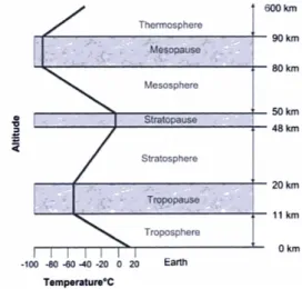
Figure 1.1: Atmospheric Layers. Source:Larry C. Andrews,Laser Beam Propa-gation Through Random Media,pg:10
The atmosphere is a gas envelope that covers the earth. It is divided into 4 primary layers and 3 isothermal boundaries. The Troposphere layer contains 75% of the earth’s atmospheric mass and maximum air temperature occurs in the near surface of the earth. The tropopause layer is an isothermal layer where the air temperature remains constant at -55 0C. In the Stratosphere layer, the
air temperature increases with altitude because of the effect of ozone where the absorbed sunlight creates heat energy. The Stratopause boundary creates an isolation layer between Mesosphere and stratosphere layers.In the Mesosphere layer, the temperature is relatively cooler and it decreases down to -900C. The Mesopause boundary is a third isothermal boundary. Finally the air temperature
in the Thermosphere layer rises significantly after 90 km and it also containes most of the Ionosphere and Exosphere. The layers of atmosphere can be seen in Figure 1.1.
All of the experiments done in this thesis have been done in the Troposhere layer, where most of the atmospheric mass is carried and most of the life we know exist.
Absorption and scattering generally refer to wavelength dependent attenu-ation of electromagnetic radiattenu-ation where in absorption, atmospheric molecules absorb energy from incident photons and in scattering, photons collide with the atmospheric molecules. In the atmosphere, H2O, CO2, CO, N O2, and
the ozone are the fundamental absorbers. Little absorption occurs at visible wavelengths(0.4 − 0.7µm ) except for H2O absorption between 0.65 µm and 0.85
µm. First order scattering, known as Rayleigh law, is caused by air molecules that are relatively smaller than the wavelength of the radiation. The scattering coefficient is proportional to λ−4, known as the Rayleigh Law. Mie Scattering is scattering with particles comparable in size to the radiation wavelength. Losses from scattering decrease abruptly as the wavelength increases .
Overall, the transmittance of a laser beam that has propagated a distance L through the atmosphere can be interpreted with the Beer’s Law :
τ = exp[−α(λ)L] (1.1)
where, α(λ) = Aa+ Sa , Aa : Attenuation coefficient and Sa : Scattering
coeffi-cient and α(λ)L is the optical depth .
As a result of some of the software packages that are commercially and freely available , we can derive the transmittance effects of a horizontal path in the atmosphere as a function of wavelength as it can bee seen in Figure 1.2. In classical theory of turbulence, atmosphere is defined in two distinct states of motion, laminar and turbulent. In laminar flow, mixing of the media does not
Figure 1.2: Typical atmospheric transmittance for 1 km horizontal path, 3 meters above the ground, no fog, no rain, no clouds. Source:Larry C. Andrews,Laser Beam Propagation Through Random Media,pg:13
occur and velocity flow characteristics of media change in a regular fashion. In turbulent flow, dynamic mixing of the media occurs and velocity flow loses its uniform characteristics. As a result of the dynamic mixing of turbulent flow random sub-flows called turbulent eddies are created. The theory assumes the small scale structure of turbulence to be statistically homogeneous, isotropic, and independent of larger scale structure.
The source of energy at larger scales is either wind shear or convection. In cascade theory of turbulence, when the wind velocity reaches a critical point, it creates unstable air masses (eddies) that are slightly smaller and independent from the initial flow. So larger eddies break up into smaller eddies and form a continuum of eddy sizes between the Lo (outer scale of turbulence) and lo (inner
scale of turbulence). An illustration is shown in Figure 1.3.
1.2
Classical Theory
In classical theory of optical wave propagation, the assumption is essentially un-bounded continuous medium with smoothly varying refractive index.Therefore
Figure 1.3: The Cascade theory of turbulence where Lo denotes the outer scale
and lo is the inner scale. Source:Larry C. Andrews,Laser Beam Propagation
Through Random Media,pg:60
assuming a monochromatic wave, the vector amplitude of the field can be de-scribed by Maxwell’s equations [2],
O2E + k2n2(R)E + 2O[E.Olog(n(R))] = 0; (1.2) where R = (x, y, z) denotes a point in space and k = 2π/λ is the wave number of the electromagnetic wave, λ is the wavelength and n(R) is the refraction index.
The main starting point for the classical theory of propagation through ran-dom media is [2],
O2U + k2n2(R)U = 0 (1.3)
where U (R) is the scalar component of the electric field. Essentially all ap-proaches for solving this equation rely on the following fundamental assumptions [2],[3],[4]:
• Backscattering of the wave can be neglected.
• The wave equation may be approximated by the parabolic equation. • The refractive index is dirac delta correlated in the direction of propagation.
The first method that agrees with the experimental data is the Rytov ap-proximation using log − normal model for irradiance. The starting point for this method is given below.
U (R) ≡ U (r, L) = U0(r, L)eψ1(r,L)+ψ2(r,L)+... (1.4)
where U0(r, L) is the unperturbed field and ψ1(r, L) and ψ2(r, L) represent first
and second order perturbations.These perturbations are explained in the nor-malized Born Approximations according to,
ψ1(r, L) = U1(r, L) U0(r, L) = Φ1(r, L), (1.5a) ψ2(r, L) = U2(r, L) U0(r, L) − 1 2[ U1(r, L) U0(r, L) ]2 = Φ2(r, L) − 1 2Φ 2 1(r, L). (1.5b)
It is interesting that even though all of the approximations that are used in Rytov theory are taken from Born approximation and Born approximation is only a way to explain extremely weak turbulence conditions, the three integrals that are given below are used to explain second and fourth order statistics in the theory of propagation through random media, where Φn(K, z) shows the nth
order spectral representation.
E1(0, 0) =< ψ2(r, L) > +12 < ψ21(r, L) > = −2π2k2RL 0 dz R∞ 0 dKKΦn(K, z) (1.6)
E2(r1, r2) =< ψ1(r1, L)ψ2∗(r2, L) > = 4π2k2RL 0 dz R∞ 0 dKKΦn(K, z)J0(K|γr1− γ ∗r 2|) ×exp[−iK2 2k (γ − γ ∗)(L − z)], (1.7) E3(r1, r2) =< ψ1(r1, L)ψ1(r2, L) > = 4π2k2R0LdzR0∞dKKΦn(K, z)J0(γK|r1− r2|) ×expd−iK2γ k (L − z)e, (1.8)
1.3
Aperture Averaging Theory
Decrease in scintillation with the increase in the receiver lens area is known as Aperture Averaging(AA). The decrease in scintillation due to aperture averaging can be reached from the ratio of power fluctuations over a defined size of aperture by a point size aperture. Assuming I(r,L) is the irradiance of an optical wave col-lected by a lens of a receiver diameter D in an FSO system, L is the propagation distance and r is the spatial vector in the transverse plane of the receiving lens, then the total power that is collected from the receiver lens P =R I(r, L)dr.
If we are dealing with an unbounded plane wave, < P >= 1
8πD
2 < I > (1.9)
where < I > is the mean irradiance .The normalized variance of power fluctua-tions in the receiver plane leads to[5],
σ2 p(D) = <P2>−<P >2 <P >2 = πD162 RD 0 bI(p)[cos −1(p D) − p D(1 − p2 D2) 2]pdp, (1.10)
where bI(p) = BI(p)/BI(0) is the normalized covariance of irradiance
fluctua-tions, p denotes the separation distance between two points on the wavefront and the terms in the brackets arise from the optical transfer function or the Mutual Transfer Function (MTF). The covariance function of the irradiance is
based on the assumption of the modulation process I = xy and the irradiance covariance function can be expressed as the sum,
BI(p) = Bx(p) + By(p) + Bx(p)By(p) (1.11)
where Bx(p) is the covariance of the large-scale fluctuations and By(p) is the
covariance of the small-scale fluctuations.
In the literature, the covariance of irradiance can also be expressed as [2][3][4],
BI(p) = eBx(p)+By(p)− 1 . (1.12)
Under weak turbulence regimes, the correlation width of the optical scintilla-tion screen is on the order of the Frensel zonepL/k [6]. However as the strength of the turbulence gets bigger, the correlation length decreases. When the long residual correlation length is considered, it is found that the correlation length can be determined by the scattering disk size kpL
0, p0 being the spatial correlation
length under strong turbulence regimes [3].
In this thesis, numerous studies are done in atmospheric optics to investigate the nature of turbulence. In chapter 2, we are focusing on several subjects; tur-bulence strength estimation from sequential images taken as output of a large aperture telescope, simulation of propagation of a turbulence induced beam in various turbulence regimes using phase screen method, turbulence strength es-timation using angle of arrival method, image acquisition algorithm which is especially useful in strong turbulence induced images and Support Vector Ma-chine (SVM)algorithm for estimating turbulence strength in weak to moderate turbulence conditions. In chapter 3, a turbulence investigation setup has been proposed and weak to strong turbulence induced beam has been investigated in various experiment sites and weather conditions. In addition, a feasible and practical method for turbulence strength estimation setup has been proposed. In
chapter 4, the experimental results that are gathered in weak to strong turbu-lence regime has been compared with the scintillation index theory, which is the most accepted theory that is in use in experimental and theoretical studies in atmospheric turbulence literature. It is seen that although there is a very good correlation with the data taken in weak to moderate regime, as the turbulence level gets stronger the error margin increases. So the literature is in need of a superior theory that will explain intensity variations of a given receiver aperture in all turbulence regimes.
Chapter 2
Simulation Model
2.1
Refractive Index Structure Constant (C
n2)
Evaluation
In turbulence theory, the fundamental problem with the processing of the image sequences is the measurement time that takes place within the turbulent me-dia. Estimating turbulence strength that is resulted by intensity fluctuations in a turbulent media is yet another challenge to get over. The path-averaged re-fractive index structure constant, Cn2, is a fundamental parameter to characterize the atmospheric turbulence. In order to measure C2
n, we need a device called a
scintillometer which processes the image in real time and needs expensive equip-ments. In this part of the thesis, we want to present a method to estimate the C2
n parameter from a turbulence induced image sequence.
Random variations in the refractive index induce multiple refractions to the wave propagating through the atmosphere. So the wave front propagating through arrives at the output plane with random phase angles whose variances
depend on the strength of the turbulence. This phenomenon has two main im-pacts at the output plane. The first one is the spatiotemporal movements in the image plane. In the practical case, the same intensity value occurs in different pixel locations across the frames. The distance between each location is directly related with the turbulence strength and a method will be presented to measure the C2
n parameter. The second one is the long exposure blur. Long exposure
blur is caused by the technique that is being used when capturing images with a camera. In a sufficiently short time exposure (up to a few milliseconds), the intensity of a single wave front with random angle of arrival can be recorded at each frame. But the cameras with sufficiently long exposure times will simply add the intensities of the wave fronts and integrate over time. So simply, the effect of ’angle of arrival’ will be averaged over the spatial domain and we will loose the knowledge of spatiotemporal movements occurring in the propagation direction.
Assuming that we have a camera with sufficiently short exposure time, the variance for turbulence induced plane wave assuming path averaged C2
n is given as [7], σ2a= D−1/3Cn2L × P (2.1) where, P = 2.914, l0 << D << √ λL 1, 1,√λL << D << L0
A wave front angular shift at α radians results in an image displacement of αxP F OV−1 where PFOV is the pixel field of view. So the image displacement in a spatial domain for the output plane is,
By filtering the image with gradient based masks, we can have the changed images in both spatial axes. A spatiotemporal, 4-point central difference for dif-ferentiation (with mask coefficients) 1/12(-1,8,0,-8,1) has been used as a mask.[3] The strength of the change is derived mostly from the size of turbulence eddies and it is directly proportional to the intensity variance as [8],
σI2(m, n) = [Ix2(m, n) + Iy2(m, n)]σimg2 (2.3) where Ix(m, n) and Iy(m, n) represent the pixel location of gradient filter result.
So overall, the intensity variance can be calculated as,
σ2I(m, n) = [Ix2(m, n) + Iy2(m, n)]D−1/3Cn2 × L × P × P F OV−2 (2.4)
The C2
n parameter can be obtained as,
Cn2(m, n) = ([Ix2(m, n) + Iy2(m, n)] × L × P )−1P F OV2D1/3σ2I(m, n) (2.5)
At the end we have found a C2
n value for each pixel of the output image. The
average is the estimated turbulence strength parameter,
Cn2 = P m,nC 2 n(m, n) m × n (2.6) The C2
nimage that is seen in Figure 2.1 represents the change in the refractive
index along the pixel path. It is observed that the results occur where the image intensity lies.
For further investigations, a scintilometer is needed to run simultaneously with our setup as we gather images. Comparing the estimated values and the gathered ones from the scintilometer will give us a chance to make a perfect estimation.
Figure 2.1: The C2
2.2
Phase Screen Method
2.2.1
Introduction
Experimenting on a free space optical communication system is rather tedious and difficult. The interferences of plentiful elements affect the result and cause the experiment outcomes to have bigger error variance margins than they sup-pose to have. Especially when we go into the stronger turbulence regimes, the simulation and analysis of the turbulence induced beams require delicate atten-tion [9]. Simulaatten-tion of the beam propagaatten-tion through a turbulent media for diverse turbulence regimes is investigated in our previous studies [10].
For all of these purposes, a method for creating turbulence effects on a prop-agated beam in a desired experimental condition for all turbulence regimes is presented in this section.
In our simulations, we have used a point source which combines the Gaussian and sinc forms in 2D [11] [12],
pgausSinc = exp(−j k 2Dz r2))Dob λDz sinc(Dob λDz x1)sinc( Dob λDz y1) (2.7)
where Dz is the propagation distance x1, y1 are the cartesian spatial coordinates,
r is the polar spatial coordinate and Dob is the diameter of the observation field
aperature.
In the act of propagation through air, a super-Gaussian absorbing boundary is applied spatially through for addition of random phase screens to the propagated beam [13]. It is useful for getting rid of the back reflections from boundary layer in propagation between two phase screens.
GSupG = exp(− 1 2( r σ) 8 ) (2.8)
where r is the location parameter of polar coordinates and σ is about the half of the number of grids (N).
For the propagation of the beam, the angular spectrum form of Fresnel diffrac-tion has been used [11],
U (r2) = F−1[r2, f1]{H(f1)F (f1, r1){U (r1)}} (2.9)
where F [r, f ] is the fourier transform and H(f ) is the transfer function of the free space propagation given as,
H(f1) = ejk∆zejπλ∆z(f
2
x1+fy12 ) (2.10)
The modified Von Karman spectrum has been chosen for its identity with the Kolmogorov spectrum when the inner scale of turbulence,l0 = 0 and outer scale
of turbulence L0 ∼= inf,
P SDmodV onKar = 0.033Cn2exp(−
(KK m) 2 (KK22 0) 11 6 ) (2.11) where Km = 5.92l0 and K0 = 2πL0
In Figure 2.2, the Modified Von Karman Spectrum vs the Von Karman Spec-trum is given. Experimental results show that the bump near 1/l0 is steeper
for the modified version of the Von Karman Spectrum so we choose it in our simulation.
Figure 2.2: Modified Von Karman Spectrum vs the Von Karman spectrum
2.2.2
Phase screen Methodology
Simulation of the beam propagation in a turbulent media is explained in the literature [11] [12] [14] [15]. In the preceding section, we offer a methodology for creating real-time turbulence like atmospheric effects on a propagated beam with a predetermined turbulence strength.
Using the point source in the form of Eq. 2.7, we have established a propa-gation pattern at a distance Dz. After defining equi-distance observation plane
locations between the source plane and the final observation plane, the same numbers of turbulence phase screens have been created to alter the phase factor of the propagated beam. The methodology for the turbulence phase screen is described in the following paragraphs.
Fast fluctuations, which are found to be the effective parameter that cause the strong turbulence, are applied to the propagated beam for each screen defined
by the Fresnel diffraction method where ∆obis the observation plane spacing and
the N is FFT factorization number.
Depending on the observation grid spacing, the frequency grid is also estab-lished,
ff ast = (−N/2 : N/2 − 1) ×
1 N × ∆ob
(2.12)
Using Eq. 2.11, we have calculated the associated power that is induced by the fast fluctuations where K = λ2π
f ast and λf ast=
c
ff ast.
In the forthcoming section, we are offering a new method for calculating the power spectrum for both slower and faster fluctuations . For turbulence regimes that are moderate to strong (σR > 1), we believe that variations of the
power fluctuations that are induced to the propagated beam gets bigger. So in the process of calculation of the power associated with each turbulence phase screen, the C2
n variation increases even after short distances. By taking the
effect of the angular spectrum form of Fresnel diffraction into account (Eq.2.9), we introduce randomness to the power that is induced to the propagated beam in each turbulence phase screen which will be effective in reaching the desired turbulence strength.
First a initial C2
n has been decided for the specific propagation path and
turbulence regime. Then the C2
n function for all turbulence regimes is introduced
for each phase screen as,
CnScrn = randn(Cn2, C 2 n×
σR2
100) (2.13)
where randn is a matlab function that generates a normal distributed random number with a mean of C2
n and a variance of Cn2 × σ2R 100.
Then normal distributed random numbers with a unity power of (NxN) size phase screen is created. For each phase screen along the propagation path, power associated for each pixel point is assigned to the appropriate planar frequency as a Fourier coefficient of the phase screen according to the power spectrum density calculated in Eq. 2.12. So at the end, we have introduced randomness not only in the spatial and temporal domains but also in the power associated with turbulence in each phase screen.
cnF ast= rand[N × N ] ×pP SDf ast× ∆ob (2.14)
The Inverse Fourier transform is taken in 2D for realizing the fast fluctuation effect of the turbulence phase screen Φhigh,
Φhigh = F−1{cnF ast} (2.15)
Resulted fast fluctuations can be seen in Figure 2.3.
Figure 2.3: Fast Fluctuation Effect of the Optical turbulence on a 100 meter slant path with a Cn2 = 10−16.
Lower fluctuations have been accomplished using the same rule applying a larger frequency grid,
flow = [−1, 0, 1] ×
1 3round(3.4/(C2×1016))
Again using Eq. 2.11, we have calculated the associated power that is induced by the lower fluctuations where K = λ2π
low and λlow =
c flow.
Then the Fourier coefficients associated with the lower fluctuations are cal-culated by,
cnLow = rand[N × N ] ×
p
P SDLow× ∆ob (2.17)
And the turbulence phase screen for lower fluctuations is found by taking an inverse Fourier transform,
ΦLow = F−1{cnLow} (2.18)
Resulted fast fluctuations can be seen in Figure 2.4,
Figure 2.4: Lower Fluctuation Effect of the Optical turbulence on a 100 meter slant path with a C2
n = 10 −16.
The addition of the two effects have created a practical turbulence screen with pre-known turbulence structure parameter (C2
n) according to Eq. 2.19 and
is given in Fig. 2.5. Using this type of addition for each phase screens we are giving a major role to the fast fluctuations in strong turbulence regimes whereas in weaker turbulence regimes this role goes to the lower fluctuations [10].
Figure 2.5: Simulation Result of Optical turbulence screen on a 100 meter slant path with a C2
n= 10 −16.
ΦT OT = ΦF ast× e−σR−1+ ΦLow (2.19)
Resulted optical turbulence screen have been collimated with each sequential observation plane. The influence of the turbulence phase screen has been passed through, while we propagate using Eq. 2.9 until the last observation plane.
2.2.3
Results
We have a perfect scintillation pattern which has a specific turbulence strength structure constant (C2
n) with a pre-defined propagation distance. In Figures
2.6-2.7, we can see the observation plane of a 633 nm beam after 100 meters of distance in various turbulence strengths.
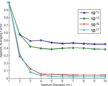
The simulation results of the Aperture Averaging factors for varying Aperture Sizes in various turbulence regimes is given in Fig. 2.8. The strong turbulence data shows itself in the saturation level of the Aperature Averaging Factor.
The experimental results and their methodology has been explained through-out Chapter 3. Experimental and simulated results of Point Averaged Aperature Averaging (PAAA) Factor for the strong turbulence regime is given in Fig. 2.9. Experimental results in the strong turbulent regime show us that the declination
Figure 2.6: Strong Turb.(Cn2 = 10−10) and Intermediate Turb.(Cn2 = 10−13) Images, Path:100 m. l0 = 5mm and L0 = 104.
Figure 2.7: Weak Turb. Image, ,Path:100 m. C2
n = 10 −15, l
0 = 5mm and
L0 = 104.
of the curve is very similar to our simulation results. There is a %10 error margin in the saturation region of the Aperture Averaging curve which is acceptable in strong turbulent regimes.
The AA Factor for weak-to-moderate turbulence regime is given in Fig. 2.10. Experimental results seem to match up with the simulation results in the satu-ration regime of the curve. It is our idea that the declination difference is caused by the number of phase screens that are in use. The difference can be decreased
Figure 2.8: Simulated Aperture Averaging Results over 100 meters for various C2
n values
by increasing the number of sampling we take from the observation plane for each realization.
In conclusion, a practical method for creating turbulence like phase screens has been established in desired turbulence regimes. The new method for estab-lishing the right measures of addition to the propagated beam has been con-structed by arranging the influence of lower and faster fluctuations. It has been found that faster fluctuations are more effective on the strong turbulent regimes. Desired turbulence strength has been established with simulation by suggest-ing temporal fluctuations in the induced turbulence power in strong turbulence conditions.
Figure 2.9: Experimental and Simulated Results of the Point Averaged Aperture Averaging Factor for C2
n = 2x10
−12, path length =120 meters, l
0 = 5mm and
L0 = 104.
Figure 2.10: Experimental and Simulated Results of the Point Averaged Aperture Averaging Factor for Cn2 = 5x10⁻¹⁴, path length =120 meters, l0 = 5mm and
2.3
Image Acquisition and Tracking Algorithm
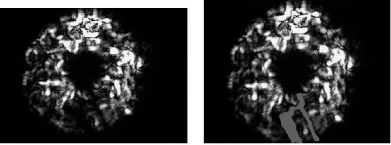
The ideal image at the receiver side without any turbulence should be seen as a perfect donut shape(Fig. 2.11). In terms of intensity distribution, we can safely approximate the same intensity value at each point (plane wave approximation) since D << √λL, where D is the receiver aperture, λ is the wavelength and L is the propagation path. Existing data from the University of Maryland setup have been used to test our software.
Figure 2.11: Intensity Distribution of the Image at the Receiver Side with no Turbulence Effects.
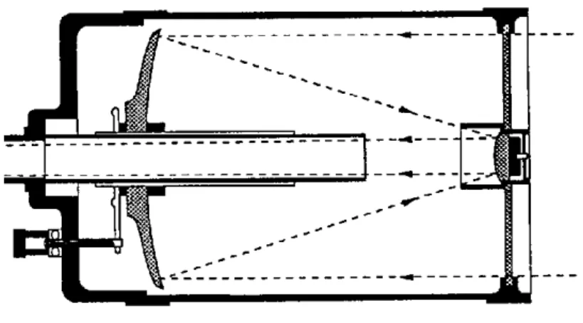
The dark area occurs in the middle because of the small diameter mirror of the Schmidt-Cassegrain telescope at the receiver side blocking the central portion of the image as shown in Figure 2.12.
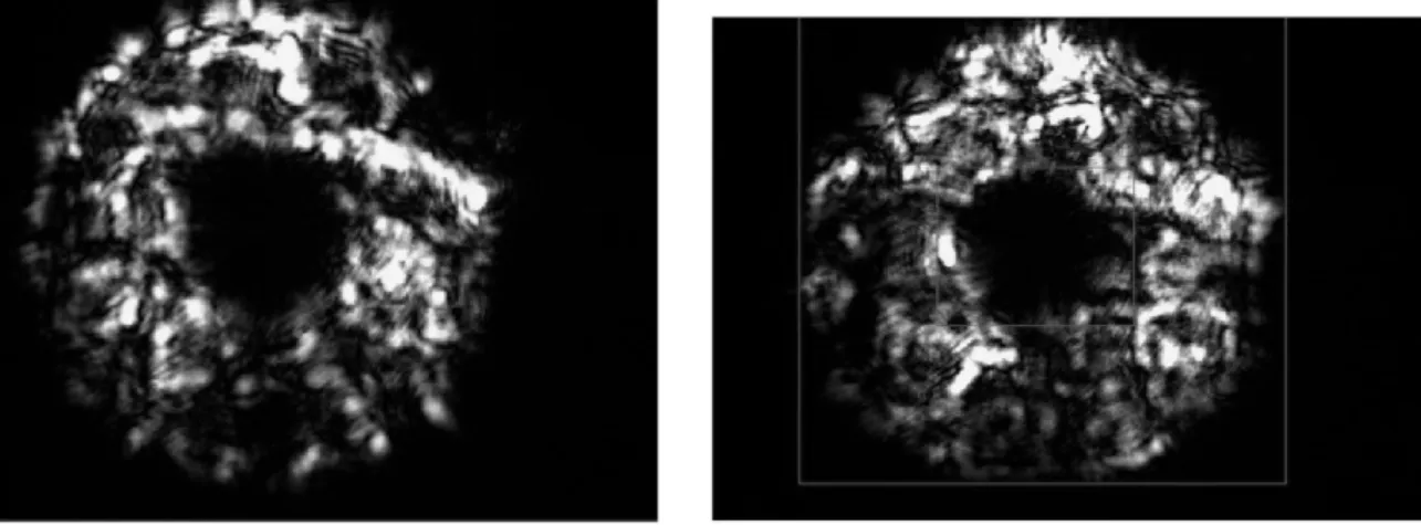
Due to turbulence induced fluctuations, the intensity distribution of the image at the receiver becomes rather plain and simple as shown in Figure 2.13.Resulted boundaries as a result of the software is shown in Figure 2.13. In order to analyze the image, we have to set some deterministic boundaries for where our informa-tion lies. Mainly we can determine these boundaries by only two parameters, radius of the inner circle and radius of the outer circle. The preceding method will explain the steps of succession in our software.
Figure 2.13: Turbulence induced image and Region result of the software
At first, we subtract the background noise, which is only one frame that is taken from the camera when the laser is off, caused by the noise that is coming from thermal radiations or sun rays. After that process, a smoothing operation is needed to reduce the effects of the turbulence generated paths from the inner circle to the outer circle. Examples of such images can be seen in Figure 2.14.
Then we convert a binary image from the result to see where our information lies. Smoothing operation gives us a better understanding of the inner and outer boundaries of the image. The difference caused by the smoothing operation can be clearly seen in Figure 2.15.
Labeling each of the closed boundaries gives us several regions inside our image matrix. The biggest one of these should be able to give us the outer
Figure 2.14: Turbulence induced problematic image and the Region that is caus-ing problems
Figure 2.15: Binary image without smoothing and Binary image after smoothing radius of the image. For the region with the biggest area, we are able to fit a square or a circle after that by calculating the minimum and maximum location points in the x-axis and the y-axis.
The same operation applies for the inner circle. The only difference is that the region of the inner circle is assumed to be higher than 1/8 of the size of the image.
Once the inner and outer radius of the captured frames are determined, the same framing technique discussed previously is used in calculating the Aperture
Averaging Factor. The better masking technique discussed above produced more efficient Aperture Averaging Factor results.
2.4
Analysis of turbulence strength for free
space optical communication using Support
Vector Machine (SVM) regression methods
2.4.1
Introduction
Free space optical(FSO) communication links have become more and more im-portant in recent years. They provide high speed, secure point to point com-munication. They have low probability of interception and low probability of detection. And of course they are favorite with their rapid deployment and flex-ible properties. The most favorite property of these systems is they are much more cheaper in comparison with to its alternative fiber optic communication links.
Unfortunately the only problem in the FSO Links is in the turbulence that occurs in the channel that is the atmospheric space between the transmitter and receiver. Accordingly, the modulation scheme changes in the sense of increas-ing the redundancy which reduces the bandwidth of the communication system. The optimum communication speed can only be decided by knowing the model of turbulence. Different models for optical transmission in different turbulence regimes exist in the literature [16]. But they all depend on a parameter, Cn2 , which basically gives us information about the strength of the turbulence.
The refractive index structure function, C2
n, is a parameter which describes
the magnitude of the turbulence effects in the atmosphere for the optical range. In order to measure it, we need a device called a scintillometer which processes the information realtime and needs expensive optical equipments. In this study, we will try to estimate Cn2 from different strengths of turbulence induced images using support vector regression methods.
2.4.2
Feature Extraction
The data consists of 10 classes with 30 patterns in each class with weak-to-strong turbulence Cn2 values. Our patterns are the images we got from our outdoor optical setup. The images are obtained by a CCD camera with a 1ms shutter speed which allows us to get the required power in our camera without much of intensity saturation. Each image has 1040 x 1393 pixels. So it is not computationally sensible to use all of the image as our feature vector. Therefore, different methods are applied in the proceeding sections.
2.4.3
Region Covariance Method
Feature selection is a critical step for classification problems. Region covariance is a fast method and has efficient algorithm. In this method, the covariance of some statistics of the image is obtained and the elements of that covariance matrix are used as features. Note that, it is assumed that covariance is enough to discriminate two different distributions. Note also that two distributions with different means but the same covariance matrices will not be classified. However, this is very unlikely to occur in practice [17]. Since the covariance is used for the feature selection, the dimensionality is reduced considerably. Due to symmetry, the covariance matrix has only d(d + 1)/2 different elements, where d is the number of dimension for each frame that belongs to a specific class. On the other hand, the raw values need (n × d) dimension which is much larger, where n is the number of frames in each class. In order to obtain the covariance matrix, pixel locations (x, y) and the first order and second order derivatives are used as the elements of the feature vector. Therefore, each pixel of the image is represented by a seven-dimensional feature vector given as [17],
F (x, y) = [x y R(x, y) |∂I(x, y) ∂x | | ∂I(x, y) ∂y | | ∂2I(x, y) ∂2x | | ∂2I(x, y) ∂2y |] (2.20)
where (x, y) is the pixel location, R is the color value and I is the intensity. The image derivatives are calculated using the filters [1 − 1]T and [−1 2 − 1]T for the first order and second orders respectively. Therefore, the covariance is obtained as a 7x7 matrix with 28 different elements. Note that, the feature can be reduced by excluding second order derivatives given in equation (2.20). In this case, the covariance matrix is obtained with 5x5 dimensions and the number of different elements is reduced to 15. In our study, the features are extracted for both cases and the results are discussed.
2.4.4
Discrete wavelet transform (DWT)
In Discrete Wavelet Transform (DWT), unlike the Fourier transform, the signal is represented in time-frequency domain. In DWT, there is a set of basis functions, called wavelet, that replace sinusoidal basis functions in the Fourier transform. The wavelets are stretched and shifted version of a fundamental real valued wavelet (mother wavelet) [18] . A wavelet is defined by a wavelet function and scaling functions. The wavelet transform is considered as very useful since they provide an efficient representation of many type signals. In this study, 1-level and 3-level wavelet transforms are applied to each image and the energy of multi-level decomposed image is used as the features. The standard deviation can be computed as [19], σk = v u u t 1 M xN M X i=1 N X j=1 (wk(i, j) − µk)2 (2.21)
where wk is the coefficient of kth multiwavelet decomposed sub-band, µk is the
mean value of the kth sub-band and MxN is the size of multiwavelet decomposed sub-band.
2.4.5
Complex Wavelet Transform
Despite its efficient computational algorithm, wavelet transforms have some shortcomings such as oscillations, shift variance, aliasing and lack of directional-ity. Instead, dual-tree complex wavelet transform which overcomes this limita-tions can be considered [18]. In this method, the complex transform of a signal is calculated using two different DWT decompositions and six sub − bands are produced at each scale. In this study, 2D-dual tree complex wavelet transform is applied and the features are extracted for level-1 to level-4.
2.4.6
Support Vector Machine Classification
The classification is done by conventional Support Vector Machine(SVM) algo-rithm using Gaussian radial basis function as kernel: exp(−gamma ∗ |u − v|2).
The dataset consists of 10 classes with 30 patterns in each class. Half of the dataset is used as training set and the other half is used as test set. SVM, mat-lab toolbox[20] have been used in this work for both classification and regression.
Class 1 1.8 ∗ 10−4 Class 2 7.5 ∗ 10−5 Class 3 3.13 ∗ 10−5 Class 4 9.71 ∗ 10−6 Class 5 6.13 ∗ 10−5 Class 6 7.81 ∗ 10−5 Class 7 4.41 ∗ 10−5 Class 8 4.29 ∗ 10−6 Class 9 3.37 ∗ 10−5 Class 10 2.15 ∗ 10−5 Table 2.1: C2
Feature Type Level Dimension Success Rate % DWT-Doubechies(N=4) 1 4 60 DWT-Doubechies(N=4) 3 10 76 DWT-biorthonal 1 4 66.67 DWT-biorthonal 3 10 75.33 Region Covariance - 12 84.67 Region Covariance - 25 82.67
Complex Wavelet Transform 1 12 90
Complex Wavelet Transform 2 24 83.33
Complex Wavelet Transform 3 36 86
Complex Wavelet Transform 4 48 88.67
Table 2.2: Success Rate and Feature Dimensions for each scenerio Classes with their C2
n Labels given in Table 2.4.6. In Table 2.4.6, we can
see that the success rates of the discrete wavelet transform for both doubechies and biorthonal filters are almost identical. Also they give us the least successful result. For the region covariance method, we can say that including the second order derivative does not improve our classification success, while the dimension increases. It is obvious from Table 2.4.6 that the complex wavelet transform gives us the best results in our trouts among our feature extraction methods.
2.4.7
SVM Regression
We have 10 classes each of them having 30 patterns. For each class, half of the randomly chosen paterns is used as a training data and the other half is used as a test data. Classes with its Cn2 values are given in Table 2.1.
For SVM regression, conventional linear regression with e-insensitive loss function have been used. Kernel type which defines the type of mapping into a high dimensional feature space in SVM’s is analyzed for each of the different features. The types of kernels are linear, polynomial, radial basis function and exponential radial basis function.
The proceeding figures are plotted by the following methodology. For each feature with its specific level of transform or specific level of derivatives, two plots have been done. The first one simply decides on a threshold value. Afterwards depending on the magnitude of the difference between the output and the real value, it is decided if the classification is done correctly or not. In the second one, the threshold is determined as the percentage of the actual C2
n parameter
of each class.
All of the SVM Regression figures are ploted for the test data set.
0 0.2 0.4 0.6 0.8 1 x 10⁻⁴ 0 0.1 0.2 0.3 0.4 0.5 0.6 0.7 0.8 0.9 1
Success Rate vs Threshold
Constant Threshold
Success Rate
linear polynomial radial basis function exponential radial basis function
Figure 2.16: SVM Regression using 1-Level Wavelet transform with biorthonal filter 10 20 30 40 50 60 70 80 90 100 0.1 0.2 0.3 0.4 0.5 0.6 0.7 0.8 0.9 1
Success Rate vs Threshold % for each class
Threshold % for each specific class
Success Rate
linear polynomial radial basis function exponential radial basis function
Figure 2.17: SVM Regression using 1-Level Wavelet transform with biorthonal filter
0 0.2 0.4 0.6 0.8 1 x 10⁻⁴ 0 0.1 0.2 0.3 0.4 0.5 0.6 0.7 0.8 0.9 1
Success Rate vs Threshold
Constant Threshold
Success Rate
linear polynomial radial basis function exponential radial basis function
Figure 2.18: SVM Regression using 3-Level Wavelet transform with biorthonal filter 10 20 30 40 50 60 70 80 90 100 0.1 0.2 0.3 0.4 0.5 0.6 0.7 0.8 0.9 1
Success Rate vs Threshold % for each class
Threshold % for each specific class
Success Rate
linear polynomial radial basis function exponential radial basis function
Figure 2.19: SVM Regression using 3-Level Wavelet transform with biorthonal filter
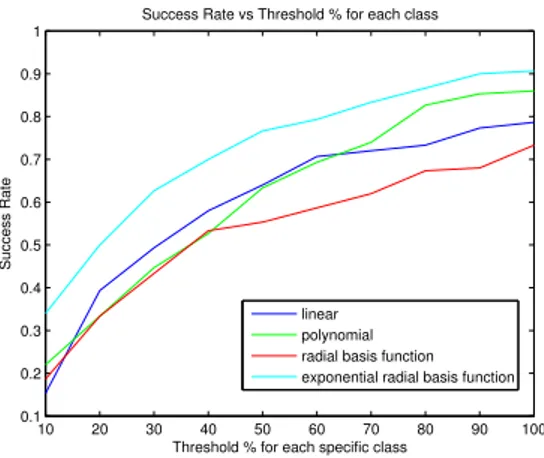
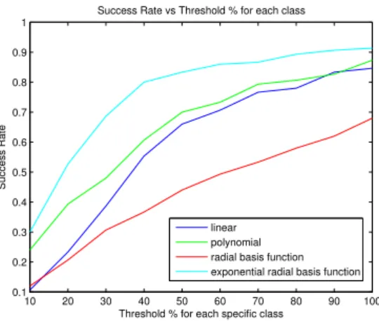
It can be seen from Figures 2.16-2.19 that the feature dimension does not really differ in the sense of success rate. Only the SVM Regression with expo-nential radial basis function seems to work better as the dimension increases in our experiment. It can be seen from Figures 2.20-2.23 that as the feature di-mension increases, the curse of didi-mensionality takes its place. It is also observed that the performance of each kernel functions are almost the same in 1-Level Wavelet Transform with doubechies filter.
0 0.2 0.4 0.6 0.8 1 x 10⁻⁴ 0 0.1 0.2 0.3 0.4 0.5 0.6 0.7 0.8 0.9 1
Success Rate vs Threshold
Constant Threshold
Success Rate
linear polynomial radial basis function exponential radial basis function
Figure 2.20: SVM Regression using 1-Level Wavelet transform with doubechies filter 10 20 30 40 50 60 70 80 90 100 0.1 0.2 0.3 0.4 0.5 0.6 0.7 0.8 0.9
Success Rate vs Threshold % for each class
Threshold % for each specific class
Success Rate
linear polynomial radial basis function exponential radial basis function
Figure 2.21: SVM Regression using 1-Level Wavelet transform with doubechies filter
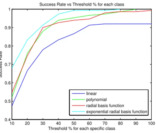
It can be seen from Figures 2.24-2.27 that the region covariance matrix feature dimension after 12 have no effect in classification. The success rate in classifica-tion has no difference as the dimensions of the feature vector increases. It is most possible that the curse of dimensionality will occur as we increase the dimensions of the features.
0 0.2 0.4 0.6 0.8 1 x 10⁻⁴ 0 0.1 0.2 0.3 0.4 0.5 0.6 0.7 0.8 0.9 1
Success Rate vs Threshold
Constant Threshold
Success Rate
linear polynomial radial basis function exponential radial basis function
Figure 2.22: SVM Regression using 3-Level Wavelet transform with doubechies filter 10 20 30 40 50 60 70 80 90 100 0.1 0.2 0.3 0.4 0.5 0.6 0.7 0.8 0.9 1
Success Rate vs Threshold % for each class
Threshold % for each specific class
Success Rate
linear polynomial radial basis function exponential radial basis function
Figure 2.23: SVM Regression using 3-Level Wavelet transform with doubechies filter 0 0.2 0.4 0.6 0.8 1 x 10⁻⁴ 0.1 0.2 0.3 0.4 0.5 0.6 0.7 0.8 0.9 1
Success Rate vs Threshold
Constant Threshold
Success Rate
linear polynomial radial basis function exponential radial basis function
Figure 2.24: SVM Regression using Region Covariance method with first order statistics
10 20 30 40 50 60 70 80 90 100 0.4 0.5 0.6 0.7 0.8 0.9 1
Success Rate vs Threshold % for each class
Threshold % for each specific class
Success Rate
linear polynomial radial basis function exponential radial basis function
Figure 2.25: SVM Regression using Region Covariance method with first order statistics 0 0.2 0.4 0.6 0.8 1 x 10⁻⁴ 0.1 0.2 0.3 0.4 0.5 0.6 0.7 0.8 0.9 1
Success Rate vs Threshold
Constant Threshold
Success Rate
linear polynomial radial basis function exponential radial basis function
Figure 2.26: SVM Regression using Region Covariance method with second order statistics 10 20 30 40 50 60 70 80 90 100 0.4 0.5 0.6 0.7 0.8 0.9 1
Success Rate vs Threshold % for each class
Threshold % for each specific class
Success Rate
linear polynomial radial basis function exponential radial basis function
Figure 2.27: SVM Regression using Region Covariance method with second order statistics
0 0.2 0.4 0.6 0.8 1 x 10⁻⁴ 0.1 0.2 0.3 0.4 0.5 0.6 0.7 0.8 0.9 1
Success Rate vs Threshold
Constant Threshold
Success Rate
linear polynomial radial basis function exponential radial basis function
Figure 2.28: SVM Regression using 1-Level Complex Wavelet transform
10 20 30 40 50 60 70 80 90 100 0.4 0.5 0.6 0.7 0.8 0.9 1
Success Rate vs Threshold % for each class
Threshold % for each specific class
Success Rate
linear polynomial radial basis function exponential radial basis function
Figure 2.29: SVM Regression using 1-Level Complex Wavelet transform
0 0.2 0.4 0.6 0.8 1 x 10⁻⁴ 0 0.1 0.2 0.3 0.4 0.5 0.6 0.7 0.8 0.9 1
Success Rate vs Threshold
Constant Threshold
Success Rate
linear polynomial radial basis function exponential radial basis function
10 20 30 40 50 60 70 80 90 100 0.1 0.2 0.3 0.4 0.5 0.6 0.7 0.8 0.9 1
Success Rate vs Threshold % for each class
Threshold % for each specific class
Success Rate
linear polynomial radial basis function exponential radial basis function
Figure 2.31: SVM Regression using 2-Level Complex Wavelet transform
0 0.2 0.4 0.6 0.8 1 x 10⁻⁴ 0 0.1 0.2 0.3 0.4 0.5 0.6 0.7 0.8 0.9 1
Success Rate vs Threshold
Constant Threshold
Success Rate
linear polynomial radial basis function exponential radial basis function
Figure 2.32: SVM Regression using 3-Level Complex Wavelet transform
Interesting complex wavelet transform effects can be seen from Figures 2.28 -2.35. In 1-3 Level transforms, with a 10% threshold for each value we have above 70% success rate with the exponential radial basis function kernel.
10 20 30 40 50 60 70 80 90 100 0.1 0.2 0.3 0.4 0.5 0.6 0.7 0.8 0.9 1
Success Rate vs Threshold % for each class
Threshold % for each specific class
Success Rate
linear polynomial radial basis function exponential radial basis function
Figure 2.33: SVM Regression using 3-Level Complex Wavelet transform
0 0.2 0.4 0.6 0.8 1 x 10⁻⁴ 0 0.1 0.2 0.3 0.4 0.5 0.6 0.7 0.8 0.9 1
Success Rate vs Threshold
Constant Threshold
Success Rate
linear polynomial radial basis function exponential radial basis function
Figure 2.34: SVM Regression using 4-Level Complex Wavelet transform
10 20 30 40 50 60 70 80 90 100 0.2 0.3 0.4 0.5 0.6 0.7 0.8 0.9 1
Success Rate vs Threshold % for each class
Threshold % for each specific class
Success Rate
linear polynomial radial basis function exponential radial basis function
2.4.8
Results and Conclusions
In this study, our main purpose was coming up with a regression method which will give us the strength of the turbulence. Since feature selection is one of the most important steps of the classification problem, we have tried three different methods which are Discrete Wavelet Transform, Complex Wavelet Transform and Region Covariance Method. As a result with the help of complex wavelet transform, we have 70% Success rate with 10% error margin and furthermore the success rate becomes above 90% with 20% error margin for each C2
n value of the
classes that are weak to moderate-to-strong induced turbulence . This accom-plishment can be used in real time FSO communication links to determine the strength of the turbulence instead of using expensive, time and power consuming bulky Scintillometers.
Chapter 3
Experimental Setup
3.1
Strong Turbulence Setup
3.1.1
Odeon Experimental Setup at Bilkent University
Existing empirical data within the weak and intermediate turbulence regimes using an 863 meters link about 1.2 meters above ground at the University of Maryland have been used to test our Aperature Averaging (AA) and image acquisition software and will be used in our model of turbulence. As it can be seen from Figure 3.1, using empirical data in intermediate turbulence conditions, the aperture averaging results demonstrate the expected reduction in intensity fluctuations with increasing aperture diameter.
The outdoor experimental setup has been completed and aligned ready for data collection at different weather conditions. The outdoor experimental loca-tion is chosen to be the Odeon Parking Lot at Bilkent University’s Main Campus. The Length of the beam path is about 250 meters. The declination of the beam path is approximately 3.420. The height of the transmitters and receivers is
Figure 3.1: Aperture Averaging Factor For Intermediate turbulence conditions
propagating beam. Figure 3.2 shows a satellite picture of the experimental lo-cation chosen for the outdoor strong turbulence experiment. The transmitter part shown in Figures 3.3 and 3.4, setup on a portable breadboard with a rigid enclosure built specially to protect the equipment and optics from the rain and severe weather conditions. Since it is a flat, open area to be used for our outdoor link, we should be expecting strong winds and heavy rain for our setup. Our setup is strong and rigid enough to bear those winds and well enclosed for the water to leak. The enclosed transmitter setup is 15 kg excluding the heavy duty tripods. A rifle scope is placed at the top of the transmitter enclosure for the use in the alignment of the beam. The Electric power is supplied from Electric utility poles that exist in the experimental area.
Figure 3.3: Enclosed Transmitter and Transmitter part front-view