ISSN 0975-8607 (online); 0976-5905 (print)
Published by RGN Publications http://www.rgnpublications.com
DOI: 10.26713/cma.v11i1.1294
Research Article
On the Solutions of Linear Fractional Differential
Equations of Order
2q
Including Small Delay
Where
0 < q < 1
Ali Demir1,*, , Kübra Karapinar1, and Sertaç Erman2, 1Department of Mathematics, Kocaeli University, Kocaeli, Turkey
2Management and Information System, Istanbul Medipol University, Istanbul, Turkey *Corresponding author: [email protected]
Abstract. The main goal of this study is to find the solutions of linear fractional differential equations
of order 2q, including small delay, where 0 < q < 1 which has various applications. The fractional derivatives are taken in the sense of Caputo which is more suitable than Riemann-Liouville sense. We assume that the order q satisfy the condition nq = 1 for some natural number n which determines the number of the linearly independent solutions. Since the delay term is small, the linear fractional differential equation is expanded in powers series of which reduce the problem to regular or singular perturbation problem for which it is easier to find the solution. The solution is obtained in the form of a series expansion of E. To demonstrate the accuracy and the effectiveness of the proposed approach, some illustrative examples are presented.
Keywords. Fractional differential; Small delay MSC. 34A08; 34K37
Received: September 11, 2019 Accepted: October 13, 2019
Copyright © 2020 Ali Demir, Kübra Karapinar and Sertaç Erman. This is an open access article distributed under the Creative Commons Attribution License, which permits unrestricted use, distribution, and reproduction in any medium, provided the original work is properly cited.
1. Introduction
Since the fractional differential equations play an important role in modelling for the wide range of problems which model systems in nature, including past memories, in various scientific research areas such as bioengineering, thermo-dynamics, viscoelasticity, control theory, aero-dynamics, electromagnetics, signal processing, chemistry, finance, it is growing considerable
interest in recent years [2, 6]. It is well known that fractional derivative is global in nature whereas the integer derivative is local in nature which makes the ODEs of fractional order intriguing topic for many scientists. This property makes fractional ODEs the best possible choice in modelling physical problems involving past memory. Since the derivatives in the Caputo sense is closer to integer order derivatives, the analysis of the ODEs involving Caputo derivatives, gives more useful results.
By making use of Mittag-Leffler function, characteristic equations of fractional ODEs are solved and solutions of them are constructed efficiently. In this sense, the Mittag-Leffler function takes the role of the exponential function which is used in the determination of solutions for ODEs with integer derivatives.
Delay differential equations (DDE’s) can be defined as the generalization of the ordinary differential equations which are appropriate for modelling physical systems with memory. The delay is an unavoidable fact of the physical systems such as transportation of energy and materials, feedback control systems kinetics, damping behavior of viscoelastic materials, so on.
The proposed approach is based on applying Taylor series expansion to simplify linear fractional differential equations with small delay. The analytical solution which is in the form of a series expansion for the linear fractional differential equations with small delay is obtained by solving the resulting regular or singular perturbation problem. In regular perturbation problems a small change in the problem causes a small change solution whereas a small change in the problem causes a large change in the solution in singular perturbation problem. Perturbation which is a local method, shows how to find the solutions approximately for the problem under the influence of the perturbation by using the solutions to the unperturbed problem [3, 10, 11].
2. Linear Fractional Differential Equations of Order
2q
, Including
Small Delay Where
0
<
q
<
1
Let us consider the following linear fractional differential equations with small delay
D2qu (t) + BDqu (t) + Cu (t) + Eu (t − ε) = 0, (1)
whereε is a small delay term. By taking advantage of this fact we expand the function including delay in the following series
u (t − ε) ≈ u (t) − εDu (t) + O(ε2).
Substituting the expansion into (1), the following linear fractional differential equations is obtained:
D2qu (t) + BDqu (t) + Cu (t) + E(u (t) − εDu (t) + O(ε2)) = 0 (2) which does not contain the function including delay. Now we assume that qn = 1 for some natural number n. Hence, we have Dt= Dtqn. By making use of this fact we can rewrite the
equation (2) in the following form:
D2qu (t) + BDqu (t) + (C + E)u (t) − EεDqnt u (t) = 0. (3)
Let u (t) = Eq,1u(rtq) be the solution of (3), then the characteristic equation for (3) is obtained
as follows [10]
after some arrangement the characteristic equation can be rewritten in the following form εrn − 1 Er 2 −B Er − µC E+ 1 ¶ = 0 , (4)
where we use perturbation theory to obtain the solution of the characteristic equation. If we have a regular perturbation problem, the solution can be represented in the following series form:
r (ε) = r0+ εr1+ O(ε2) (5)
At this stage, we consider the various cases by using the assumption:
Case 1: n = 1
Let us consider the case n = 1 which makes the characteristic equation (4)
εr − 1 Er 2 −B Er − µC E+ 1 ¶ = 0 . Arranging this equation, we get
r2+ (B − Eε) r + (C + E) , (6)
where we have regular perturbation problem which means that we seek the solution in the form of (5). Substituting (5) into (6), we get
r20+ 2εr0r1+ ε2r21+ Br0+ Bεr1− Eεr0− Eε2r1+ C + E + O(ε3) = 0. (7) Equating to zero the successive terms of the series on the left-hand side of (7):
ε0: r2 0+ Br0+ C + E = 0 ε1: 2r 0r1+ Br1− Er0= 0 ⇒ r1= Er0 2r0+ B
Solving the first equation above we have r+,−0 =−B ±
p
∆
2 ,
where ∆= B2− 4(C + E).
Similarly, for the second equation we obtain r+,−1 = E³−B± p ∆ 2 ´ 2³−B± p ∆ 2 ´ + B = E³−B± p ∆ 2 ´ ±p∆ .
Hence the approximate solution of characteristic equation becomes r+(ε) = r+0+ εr+1+ O(ε2) =−B + p ∆ 2 + ε E³−B+ p ∆ 2 ´ p ∆ + O(ε 2 ), r−(ε) = r−0+ εr−1+ O¡ ε2 ¢ = −B − p ∆ 2 + ε E ³ B+p∆ 2 ´ p ∆ + O(ε 2 ).
As a result, the approximate solution of the equations of linear fractional differential equations with small delay can be obtained in the series form of ε as follows:
u (t,ε) = α1E1,1¡r+(ε) t¢ + α2E1,1(r−(ε)t), where Eq,1(r (ε) t) = ∞ X k=0 (r (ε) t)k Γ(k + 1).
Case 2: n = 2
Let us consider the case n = 2 which makes the characteristic equation (4)
εr2 −1 Er 2 −B Er − µC E+ 1 ¶ = 0 . Arranging this equation, we have
µ ε − 1 E ¶ r 2 −B Er − µC E+ 1 ¶ = 0 , (8)
where we have a regular perturbation problem which means that we seek the solution in the form of (5). Substituting (5) into (8), we get
[r20+ 2εr0r1+ ε2r21+ O(ε3)] µ ε − 1 E ¶ − [r0+ εr1+ O(ε2)] B E− µC E+ 1 ¶ = 0 . (9)
Equating to zero, the successive terms of the series on the left-hand side of (9):
ε0 : r20+ Br0+ C + E = 0 ε1: r2 0− 1 E2r0r1− B Er1= 0 ⇒ r1= Er20 2r0+ B
Solving the first equation above r+,−
0 =
−B ±p∆
2 ,
where ∆= B2− 4(C + E).
Similarly, for the second equation we obtain r+,− 1 = E³−B± p ∆ 2 ´2 2³−B± p ∆ 2 ´ + B = E³−B± p ∆ 2 ´2 ±p∆ .
Hence the approximate solution of characteristic equation becomes r+(ε) = r+0+ εr+1+ O(ε2) =−B + p ∆ 2 + ε E ³ −B+p∆ 2 ´2 p ∆ + O(ε 2 ), r−(ε) = r−0+ εr−1+ O(ε2) = −B −p∆ 2 − ε E³B+ p ∆ 2 ´2 p ∆ + O(ε 2.
As a result, the approximate solution of the equations of linear fractional differential equations with small delay can be obtained in the series form of ε as follows
u (t,ε) = α1E1 2,1 ³ r+(ε) t12 ´ + α2E1 2,1(r −(ε)t12), where E1 2,1 ³ r (ε) t12 ´ = ∞ X k=0 (r (ε) t12) k Γ(12k + 1). Case 3: n = 3
Let us consider the case n = 3 which makes the characteristic equation (4)
εr3 −1 Er 2 −B Er − µC E+ 1 ¶ = 0 (10)
which is a singular perturbation problem. Both by seeking the roots in the form of (5) and by scaling r = εbx and balancing the suitable terms to recover the solutions of equation (10)
Substituting (5) into (10), we obtain ε[r3 0+ 3εr 2 0r1+ O(ε2)] − 1 E[r 2 0+ 2εr0r1+ O(ε2)] − B E[r0+ εr1+ O(ε 2 )] − µC E+ 1 ¶ = 0 . Equating to zero, the successive terms of the series:
ε0: r2 0+ Br0+ C + E = 0 ε1: Er3 0− 2r0r1− Br1= 0 ⇒ r1= Er30 2r0+ B
Solving the first equation above r+,−0 =−B ±
p
∆
2 ,
where ∆= B2− 4(C + E)
Similarly, for the second equation we obtain r+,−1 = E³−B± p ∆ 2 ´3 2³−B± p ∆ 2 ´ + B = E³−B± p ∆ 2 ´3 ±p∆ .
Hence the approximate roots of characteristic equation becomes r1(ε) = r+0+ εr+1+ O(ε2) =−B + p ∆ 2 + ε E³−B+ p ∆ 2 ´3 p ∆ + O(ε 2 ), r2(ε) = r−0+ εr−1+ O(ε2) = −B −p∆ 2 + ε E³B+ p ∆ 2 ´3 p ∆ + O(ε 2).
Let us find the root in the following form
r3(ε) = εbx . (11)
Substituting (11) into (10), we have Eε3b+1x3− ε2bx2− Bεbx − C − E = 0.
In order to find b, examine the three possible pairs of terms. If we balanceε2b= εb, we find b = 0 recover the first root above. If we balance ε3b+1= εb, we find b = −12, but the termε2b is the dominant term cannot be balanced by either of the other two terms. Finally, if we balance
ε3b+1= εb
, we find b = −1. Substituting b = −1
Eε−2x3− ε−2x2− Bε−1x − C − E = 0. Let us times withε2both of equation
Ex3− x2− Bεx − ε2(C + E) = 0, (12)
x(ε) = x0+ εx1+ O(ε2). (13)
Substituting (13) into (12), we have
Ex30+ 3Ex20x1− x02− 2εx0x1− Bεx0+ O(ε2) = 0. (14)
Equating to zero, the successive terms of series on the left-hand side of (14)
ε0: Ex3
ε1
: −3Ex20x1− 2εx0x1− Bεx0= 0
Solving the first equation above, we have x0= 1
E, x0= 0 .
Similarly, solving the second equation above for x06= 0, we obtain
x1=
B 3Ex0− 2
and it is clear that x1= B
for x0=E1. Therefore, an approximate solution of characteristic equation becomes
x (ε) = 1
E+ εB + O(ε
2
). (15)
Substituting (15) into (11), we have r3(ε) =1
ε
1
E+ B + O(ε
2).
As a result, the approximate solution of the equations of linear fractional differential equations with small delay can be obtained in the series form of delay termε as follows
Let r1(ε), r2(ε), r3(ε) denote the solutions of equation (10). Hence, the approximate solution
of the equations of linear fractional differential equations with small delay can be obtained as a linear combination of corresponding Mittag-Leffler functions as follows:
u (t,ε) = α1E1 3,1 ³ r1(ε) t13 ´ + α2E1 3,1 ³ r2(ε) t13 ´ + α3E1 3,1 ³ r3(ε) t13 ´ , where E1 3,1 ³ r (ε) t13 ´ = ∞ X k=0 (r (ε) t13) k Γ¡1 3k + 1 ¢.
3. Illustrative Examples
In this section, various examples are illustrated for the three cases above to show that how this method is effective and accurate.
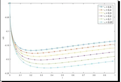
Example 1. Let us consider the following linear fractional differential equation with small
delay
D1u (t) + 3D12u (t) + u (t) + u(t − ε) = 0,
where u (0) = 0 and D12u (0) = 1.
After using Taylor Series expansion and some arrangement we have (1 − ε)D1u (t) + 3D12u (t) + 2u (t) = 0.
Hence, the solution can be represented in the following form: u (t,ε) = µ 1 1 + 5ε ¶ E1 2,1 ³ (−1 + ε)t12 ´ − µ 1 1 + 5ε ¶ E1 2,1((−2 − 4ε)t 1 2). (16)
Figure 1. Graph for the solution (16) whenε= 0.5, 0.4, 0.3, 0.2, 0.1, 0.01
Example 2. Let us consider the following linear fractional differential equation with small
delay
D1u (t) + 2D12u (t) + u (t) + u(t − ε) = 0,
where u (0) = 0 and D12u (0) = −1.
After using Taylor Series expansion and some arrangement, we have (1 − ε)D1u (t) + 2D12u (t) + 2u (t) = 0.
Hence, the solution can be represented in the following form: u (t,ε) = i 2E12,1 ³ (−1 − ε + i)t12 ´ − i 2E12,1((−1 − ε − i)t 1 2), (17) where i2= −1.
The graph of the solution u(t,ε) is given in Figure 2 for ε = 0.5,0.4,0.3,0.2,0.1,0.01.
Example 3. Let us consider the following linear fractional differential equation with small delay D23u (t) + 3D 1 3u (t) + u (t) + u(t − ε) = 0, where u (0) = 0, D13u (0) = −1 and D23u (0) = 1.
After using Taylor Series expansion and some arrangement we have D23u (t) + 3D
1
3u (t) + 2u (t) − εD1u(t) = 0.
Hence, the solution can be represented in the following form: u (t,ε) = α1E1 3,1 ³ (−1 − ε)t13 ´ + α2E1 3,1 ³ (−2 − 8ε) t13 ´ + α3E1 3,1 µµ 1 ε+ 3 ¶ t13 ¶ , (18) where α1= 8ε 2 − 2ε − 1 7ε3+ 29ε2+ 11ε + 1,α2= −ε2+ 3ε + 1 (7ε + 1)(8ε2+ 5ε + 1) andα3= −9ε3− 2ε2 (ε2+ 4ε + 1)(8ε2+ 5ε + 1).
The graph of the solution u(t,ε) is given in Figure 3 for ε = 0.5,0.4,0.3,0.28,0.25,0.2,0.15.
Figure 3. Graph for the solution (18) whenε= 0.5, 0.4, 0.3, 0.28, 0.25, 0.2, 0.15
Example 4. Let us consider the following linear fractional differential equation with small
delay D23u (t) − D 1 3u (t) − u (t) + u(t − ε) = 0, where u (0) = 0, D13u (0) = −1 and D 2 3u (0) = 1.
After using Taylor Series expansion and some arrangement we have D23u (t) − D
1
3u (t) − εD1u(t) = 0.
Hence, the solution can be represented in the following form: u (t,ε) = α1+ α2E1 3,1 ³ (1 + ε) t13 ´ + α3E1 3,1 µµ1 ε− 1 ¶ t13 ¶ , (19) where α1=−ε 2 − ε − 1 ε2− 1 ,α2= 1 (ε + 1)(ε2+ 2ε − 1) andα3= ε3 − 2ε2 (ε + 1)(ε2+ 2ε − 1) for ε 2+ 2ε − 1 6= 0.
The graph of the solution u(t,ε) is given in Figure 4 for ε = 0.5,0.4,0.3,0.2,0.1,0.15.
Figure 4. Graph for the solution (19) whenε= 0.5, 0.4, 0.3, 0.2, 0.1, 0.15
4. Conclusion
In this research, analytic or approximate solutions of linear fractional differential equations of order 2q with small delay is obtained in terms of Mittag-Leffler function, where 0 < q < 1. The fractional derivatives are taken in the sense of Caputo which is more suitable than Riemann-Liouville sense. Since delay is small, taking power series expansion of delayed term into account, the problem is reduced into a problem of regular or singular perturbation problem for which it is easier to obtain under the assumption n · q = 1 for some natural number n. Therefore the solution is obtained in the form of a series expansion of small delay. It is observed that in regular perturbation problems a small change in the problem causes a small change solution whereas a small change in the problem causes a large change in the solution in singular perturbation problem. The illustrative examples demonstrate the accuracy and the effectiveness of the proposed approach. The obtained results imply that analytic or approximate solutions of much more complicated fractional delay differential equations could be obtained by improving the method applied in this research.
Competing Interests
The authors declare that they have no competing interests.
Authors’ Contributions
All the authors contributed significantly in writing this article. The authors read and approved the final manuscript.
References
[1] A. Atangana and D. Baleanu, New fractional derivatives with non-local and non-singular
kernel: Theory and application to heat transfer model, Thermal Science 20 (2016), 763 – 769, DOI: 10.2298/TSCI160111018A.
[2] A. Atangana and I. Koca, New direction in fractional differentiation, Mathematics in Natural Science 1 (2017), 18 – 25, DOI: 10.22436/mns.01.01.02.
[3] C. M. Bender and S. A. Orszag, Advanced Mathematical Methods for Scientists and Engineers: Asymptotic Methods and Perturbation Theory, McGraw-Hill Book Company, New York (1978), DOI: 10.1007/978-1-4757-3069-2.
[4] A. Demir and E. Ozbilge, Analysis of the inverse problem in a time fractional parabolic equation with mixed boundary conditions, Boundary Value Problems 2014 (2014), Article number 134, DOI: 10.1186/1687-2770-2014-134.
[5] A. Demir, F. Kanca and E. Ozbilge, Numerical solution and distinguishability in time
fractional parabolic equation, Boundary Value Problems 2015 (2015), Article number 142, DOI: 10.1186/s13661-015-0405-6.
[6] A. Demir, S. Erman, B. Özgür and E. Korkmaz, Analysis of fractional partial differential
equations by Taylor series expansion, Boundary Value Problems 2013 (2013), Article number 68, DOI: 10.1186/1687-2770-2013-68.
[7] F. Huang and F. Liu, The time-fractional diffusion equation and fractional advection-dispersion equation, The ANZIAM Journal 46 (2005), 317 – 330, DOI: 10.1017/S1446181100008282.
[8] A. A. Kilbas, H. M. Srivastava and J. J. Trujillo, Theory and Applications of Fractional Differential Equations, North-Holland Mathematics Studies 204 (2006), 1 – 523,https://www.sciencedirect. com/bookseries/north-holland-mathematics-studies/vol/204.
[9] I. Podlubny, Fractional Differential Equations, Academic Press, New York (1999).
[10] B. Sambandham and A.S. Vatsala, Basic results for sequential Caputo fractional differential equations, Mathematics 3 (2015), 76 – 91, DOI: 10.3390/math3010076.
[11] J. G. Simmonds and J. E. Mann Jr., A First Look at Perturbation Theory, 2nd ed., Dover Publications, Mineola, New York (1998).