Vehicle classification using magnetic sensor data

(1)

KADİR HAS UNIVERSITY SCHOOL OF GRADUATE STUDIES

DEPARTMENT OF ENGINEERING AND NATURAL SCIENCES COMPUTER ENGINEERING

VEHICLE CLASSIFICATION USING MAGNETIC

SENSOR DATA

MUSTAFA SAİD UÇAR

MASTER’S THESIS

(2)

VEHICLE CLASSIFICATION USING MAGNETIC

SENSOR DATA

MUSTAFA SAİD UÇAR

MASTER’S THESIS

Submitted to the School of Graduate Studies of Kadir Has University in partial fulfillment of the requirements for the degree of Master’s in Computer Engineering

(3)

(4)

(5)

ABSTRACT

Advancements in computational power allow us to create more complex systems to solve various complicated problems. Considering numerical sensor values, computers are able to process more and more data compared to humans. Computer-based systems provide useful statistics, and predictions for problems and helps us to solve our problems in daily life.

Automated vehicle classification plays an important role in City Environmental Planning and will play an even more important role when the Self-Driving Vehicles increased in traffic. Experiments on several different sensor and camera systems are ongoing. In this study, we collect magnetic field sensor data of passing vehicles and created two datasets. Multi-class classification algorithms using Neural Networks developed and key parameters are compared. Also, popular Machine Learning al-gorithms also trained and evaluated. The main contribution of this research is data collection; the creation of a dataset for further research and development.

Keywords: Vehicle Classification, Magnetic Field Sensor, Multi Class Classifica-tion, Neural Network, Machine Learning

(7)

MANYET˙IK SENS ¨OR VER˙IS˙I ˙ILE ARAC¸ SINIFLANDIRMA

¨

OZET

Bilgisayarların hesaplama gücündeki artı¸s her gecen gün daha zor problemlerin ¸cözümünü kolayla¸stırmaktadır. Özellikle numerik sensör verileri dü¸sünüldü˘günde in-san ile kıyaslanıldı˘gında, bilgisayarlar tartı¸smasız daha fazla veri i¸sleme kapasitesine sahip. Bilgisayar tabanlı sistemler, uygun modeller ve veri setleri kullanıldı˘gında, günlük hayattaki problemlerimizi ¸cözmektedirler.

Otomatize edilmi¸s ara¸c sınıflandırma sistemleri hem S¸ehirlerin ¸cevre düzenlemelerinde, yol planlamalarında önemli bir rol oynamaktadır. Ç e¸sitli sensörler ve kamera sistem-leri kullanılarak devam eden ¸calı¸smalar halen yapılmakta. Bu ¸calı¸smada, ara¸cların manyetik alan verisi toplanıldı, i¸saretlendi ve 2 farklı veri seti olu¸sturuldu. Her iki veri seti, ¸ce¸sitli Makine Ö˘grenmesi ve Sinir A˘gları modelleriyle e˘gitildi ve sonu¸cları kıyaslandı. Bu ¸calı¸smada yapılan katkı, ileriki ¸calı¸smalarda da kullanılmak üzere veri seti olu¸sturulmasıdır.

Anahtar Sözcükler: Sözcükler:Ara¸c Sınıflandırma, Manyetik Alan Sensörü, Ç ok sınıflı sınıflandırma, Sinir A˘gları, Makine Ö˘grenmesi

(8)

ACKNOWLEDGEMENTS

I would like to thank my thesis advisor Asst. Prof. Eliya B ÜY ÜKKAYA, Asst. Prof. Figen ÖZEN, Asst. Prof. Bahar DEL˙IBAS¸ and Aylin TOKUÇ who helped me to fully accomplish this project and supported me in my relentless quest for knowledge.

I would like to also extend my gratitude to GOHM Electronics and Software for supporting me and providing essential equipment during my research.

Last but not the least, I must express my very profound gratitude to my parents and my closest friends Giray BALCI, Berkay GENC¸ and Alp Atakan ˙IS¸BAKAN for providing me with unfailing support and continuous encouragement throughout my years of study and through the process of researching and writing this thesis.

(9)

LIST OF TABLES

Table 3.1 Class distribution of dataset . . . 18

Table 3.2 15 new feature set . . . 18

Table 4.1 Grid Search Parameters . . . 21

Table 5.1 Dataset I - ML Algorithm Results . . . 35

(10)

LIST OF FIGURES

Figure 1.1 Earth’s magnetic field distortion caused by vehicle . . . 3

Figure 3.1 GOHM’s EMFU within case . . . 10

Figure 3.2 Electronic Circuits of EMFU . . . 10

Figure 3.3 Raw magnetic field records . . . 10

Figure 3.4 Dataset Label UI Home Page . . . 11

Figure 3.5 Dataset Label UI Marked Page . . . 12

Figure 3.6 Dataset Label UI Crop Page . . . 15

Figure 3.7 Dataset Label UI Trim Page . . . 15

Figure 3.8 Vehicle Signature Class Distribution . . . 15

Figure 3.9 Vehicle signature with Earth magnetic field . . . 16

Figure 3.10 Vehicle signature without Earth magnetic field . . . 16

Figure 3.11 SUV class samples energy scores . . . 17

Figure 3.12 SUV class samples outlier probabilities . . . 17

Figure 4.1 Neural network structure . . . 20

Figure 4.2 Rectified Linear Unit Function . . . 21

Figure 4.3 Example of ROC AUC plot . . . 23

Figure 5.1 Activation functions distribution on AUC Micro score in Dataset 1 26 Figure 5.2 Activation functions distribution on AUC Macro score in Dataset 1 . . . 27

Figure 5.3 Activation functions distribution on AUC Micro score in Dataset 2 27 Figure 5.4 Activation functions distribution on AUC Macro score in Dataset 2 . . . 28

Figure 5.5 Optimizer functions distribution on AUC Micro score in Dataset 1 28 Figure 5.6 Optimizer functions distribution on AUC Macro score in Dataset 1 29 Figure 5.7 Optimizer functions distribution on AUC Micro score in Dataset 2 29 Figure 5.8 Optimizer functions distribution on AUC Macro score in Dataset 2 30 Figure 5.9 Hidden Layer distribution over AUC Micro scores with first dataset 30 Figure 5.10 Hidden Layer distribution over AUC Macro scores with first dataset . . . 31

(11)

Figure 5.11 Hidden Layer distribution over AUC Micro scores with second dataset . . . 31 Figure 5.12 Hidden Layer distribution over AUC Macro scores with second

dataset . . . 32 Figure 5.13 Dropout distribution over AUC Micro scores with first dataset . 32 Figure 5.14 Dropout distribution over AUC Macro scores with first dataset . 33 Figure 5.15 Dropout distribution over AUC Micro scores with second dataset 33 Figure 5.16 Dropout distribution over AUC Macro scores with second dataset 34 Figure 5.17 First Dataset, ReLu activation, SGD Optimizer accuracy graph

of 50 epoch . . . 34 Figure 5.18 Second Dataset, elu activation, Nadam Optimizer accuracy graph

of 50 epoch . . . 34 Figure 5.19 Gaussian NB Confusion Matrix on Dataset 1 . . . 36 Figure 5.20 Gaussian NB Confusion Matrix on Dataset 2 . . . 37

(12)

LIST OF SYMBOLS/ABBREVIATIONS

Xi x-axis magnetic field vector of ith vehicle signature

xij jth x-axis magnetic field value of ith vehicle signature

Yi y-axis magnetic field vector of ith vehicle signature

yij jth y-axis magnetic field value of ith vehicle signature

Zi z-axis magnetic field vector of ith vehicle signature

zij jth z-axis magnetic field value of ith vehicle signature

RF Radio Frequency

TI Texas Instruments

NXP NXP Semiconductors

EMFU Embedded Magnetic Field Unit

SVM Support Vector Machine

C-SVM Clustering Support Vector Machine

DFT Discrete Furier Transform

PCA Principal Component Analysis

PSO Particle Swarm Optimization

NN Neural Network

ML Machine Learning

ANN Artificial Neural Network

FFNN Feed Forward Neural Network

BP-ANN Back Propagation Artificial Neural Network

KNN K-nearest Neighbor

ROC Receiver operating characteristic

AUC Area under the curve

(13)

1. INTRODUCTION

Automated vehicle detection and classification is an important problem for traffic monitoring, analysis, and infrastructure planning. Automated systems are deployed to identify the presence and type of vehicles without human interaction. There are different use cases, such as measuring traffic density, generating statistics, traffic light scheduling, automated toll collection, and planning road maintenance.

In the literature, various approaches are adopted to solve the vehicle classification problem. Many researchers used image data collected from surveillance cameras or other video sources. Although there are studies with high accuracy and efficiency, it is known that video cameras are prone to weather conditions and have high maintenance costs.

There are various studies on vehicle classification problem, relying on data collected from different types of sensors such as loop detector, sonar, radar or magnetic sen-sors.

Advancements in technology make field sensors very cheap and highly accessible; eliminating the power consumption and maintenance costs of surveillance cameras.

In this study, a single 3-axis magnetic field sensor data is used to record magnetic field changes created by passing vehicles. Figure 1.1 shows the Earth’s magnetic field distortion caused by passing vehicle in three step. Magnetic field values change if there is ferromagnetic mass around the magnetic sensor regarding the amount of the mass. Therefore, removing Earth’s magnetic field from sensor readings gives the vehicles magnetic field distortion. Since Earth’s magnetic field changes regarding the temperature, location on earth and other environmental factors, average

(14)

mag-netic field for each axis is calculated before each recording. Then while labelling samples, these average values removed from the original sensor readings using equa-tion 1.1 where xij is the jth feature of ith sample’s x-axis and avgxi is the earth’s corresponding magnetic field at that location.

xij = xij − avgxi yij = yij − avgyi zij = zij − avgzi

(1.1)

Collected magnetic field signatures of vehicles were used to create two different datasets. Then various machine learning classification algorithms and neural net-works are trained using these datasets. The objective of this research is to evaluate the Neural Network parameters and Machine Learning algorithms for each dataset regarding their performances. The effect of activation functions, optimizer func-tions and the number of hidden layers on Neural Networks are investigated and compared regarding micro and macro area under the ROC curves. Well-known Ma-chine Learning algorithm trained and compared regarding F1 and Cohen Cappa’s scores.

The organization of this study is as follows: In the following section, a literature sur-vey about vehicle classification problem is presented. Next section, data collection, contains the steps for vehicle signature extraction and preprocessing of the dataset. Then built neural network models and applied other machine learning algorithms described in the following section. Lastly, the results are discussed and concluded.

(15)

(16)

2. RELATED WORK

Monitoring and tracking data for Traffic Management Systems is an active research area. Experiments on several different sensor and camera systems are ongoing. Computer Vision based traffic monitoring systems count the passing vehicles and classify them as well as detecting lane changes. On the other hand, sensor-based systems aim to extract vehicle characteristic in order to classify a passing vehicle.

A vision-based classification algorithm is presented in (Gupte et al. 2002). Using a stationary camera, traffic scenes were recorded. Then segmentation is applied to extract vehicles from the background. After extracting the vehicle, five image processing steps are applied to the images recorded to classify vehicle. Not only that all these steps are challenging, but also maintaining the algorithms to give good result under different environments (such as day, night, rainy, foggy) makes such system not practical for successful applications.

Hussain and Moussa presented a range sensor based vehicle classification system in (2005). A range sensor is placed on top of the road to create laser intensity images. Using generated images, the following parameters are calculated; length, maximum width, maximum height, speed and average of the percent of edge points of vehicles. Authors used a Feed Forward Neural Network (FFNN) with one hidden layer. The proposed two-layer Neural Networks are trained using back propagation with a new activation function. Vehicles are classified under motorcycle, passenger car, pick-up or van, single unit truck of bus and tractor-trailer. Although the final success of the classifier seems successful, placing a vision-based sensor outdoor has its own difficulties. Environmental effects should always be monitored to make the system reliable.

(17)

In 2014, a different approach was applied to the vehicle classification problem (Ma et al. 2014). A wireless sensor based vehicle classification prototype system proposed. The system consists of 3 magnetometers to calculate the speed of the vehicle, and 6 accelerometers to count peaks and measure the distance between vehicle axles using calculated speed. Calculated variables are then converted to an image that has time in the x-axis and the peak acceleration of accelerometer in the y-axis. Although the authors did not provide the details of the algorithm they used, the proposed system has another problem. It is not applicable for a big dataset and needs special algorithms for the peak traffic time.

Due to scalability and deployment issues of image recording systems, sensor-based systems are also adapted to monitor and classify vehicles in the traffic. Such systems are cheaper to deploy and less prone to weather conditions than the surveillance cameras. Moreover, data processing cost is also much lower compared to computer-vision based systems.

Data Collection is the first challenge in a sensor based traffic monitoring system. Almost all studies collect sensor readings with the same setup in practice. An RF communication (such as wi-fi, GSM, Bluetooth, ZigBee) capable wireless sensor or a sensor network is placed on the road and the measurements are sent to a remote computer over the wireless connection. However, there are different approaches to extract vehicle signature from continuous sensor readings. Vehicle detection al-gorithm to automate vehicle detection for magnetic field sensor data is proposed (Markevicius et al. 2016). On the other hand, an acoustic sensor with accelerome-ter and a magnetomeaccelerome-ter to timestamp vehicle activity is studied in (Ng et al. 2009). Since both techniques add extra complexity and cost to the system, using a simple camera to timestamp vehicle activity is another convenient approach. During the data collection phase, a video camera is also placed on the road to record vehicle activities with timestamp alongside with the sensor values. Then, using the camera recordings, vehicle signatures are to be extracted from the raw sensor values to make the dataset more reliable.

(18)

After the collection of data, signal processing step should be applied to raw sensor readings. The most common signal processes required to be applied to raw sensor readings are removing the earth magnetic field. Since the Earth has a magnetic field and it varies from point to point, background signal should be removed to be able to extract vehicles magnetic field characteristics as explained in (Xu et al. 2017). Filter subtracts the raw signal values from the recorded vehicle signal values.

Combining data mining techniques such as feature extraction and feature selection would improve the results of classification algorithms. There are various studies in the literature addressing the vehicle classification problem using magnetic sensor datasets.

Tafish et al. used Support Vector Machine (SVM) classification algorithm to classify vehicles based on a single magnetometer sensor data (2016). As SVM is a binary classifier, they had to use two SVMs in a one-versus-all fashion to distinguish between three classes of vehicles. The proposed classification system uses Discrete Fourier Transform (DFT) and Principal Component Analysis (PCA) to automatically ex-tract features from magnetic signatures and classify vehicles into three categories. Their total classification accuracy is 87% on 1985 observations.

In 2012, a clustering algorithm based on Clustering Support Vector Machines (C-SVM) is proposed (He et al. 2012). They used binary decision trees where two kinds of vehicle types are classified in every step. To prepare input data, they transformed waveform data to numeric data using data fusion techniques. Then they used a Filter-Filter-Wrapper Model for feature subset selection. Finally, they improved the C-SVM model by Particle Swarm Optimization (PSO) for hyper parameter optimization. Ten-fold cross-validation is used to measure the accuracy of models in this work. The proposed vehicle classification method has a rate of accuracy about 99.07%, which is higher than that of the Back Propagation Artificial Neural Network (BP-ANN), the Fuzzy Discrimination (FD) and the K-nearest neighbour (KNN) classifiers applied to the same dataset consisting of 460 data points.

(19)

The authors used a simple classifier based on a hierarchical tree methodology. The vehicles are classified into motorcycles, two-box cars, saloon cars, buses, and Sport Utility Vehicle commercial vehicles (Yang & Lei 2015). They obtained over 90% classification rate for five classes of vehicles on two different speed intervals.

Kleyko et al. compared the use of logistic regression, neural network, and support vector machine algorithms to classify vehicles (2015). The dataset consists of 3074 measurements of road surface vibrations and magnetic field disturbances caused by vehicles containing five non-parametric features derived. Two layers of binary classifiers are adapted in a one-versus-all architecture. Neural Network consists of a 6-unit input layer, 3-unit output layer, and a 25-unit hidden layer. SVM uses a linear kernel. The best result of 93.4% overall classification rate is obtained by Logistic Regression algorithm.

(Ng et al. 2009) aims to find the travel direction of a car and type of vehicle as light, medium and heavy. A Neural Network is used for classification. Their test data consisted of 150 samples, 50 from each class. They achieved %100 accuracy for medium vehicles, and 70-to-80% accuracy for light and heavy vehicles. Overall, the vehicle type classifier achieved 90% accuracy in determining the classes of vehicles.

A technique of artificial neural networks (ANNs) is applied to the recognition of seismic signals for vehicle classification due to ANN’s pattern recognition capability (Lan et al. 2004). A new learning algorithm named “improved BP” is put forward to overcome BP algorithm not being fast to converge and to reach possible local minimum points. The recognition rate to gasoline engine vehicle, heavy diesel engine vehicle, and diesel engine vehicle, respectively, are 96%, 84%, and 82%. ANN is capable to solve the problem of classification and recognition of moving vehicle targets.

Another Neural Network based approach was proposed (Jeng & Ritchie 2008). Au-thors had two datasets, containing data collected by a sensor and two sensors. They proposed a model based on multi-layer perceptron neural network for single sensor

(20)

case. The deployed classifier distinguished single-unit and multi-unit trucks with 93.5% accuracy. However, the neural network did not perform well for multi-sensor dataset, due to the input data being imbalanced. Instead, they combined K-means Clustering and Discriminant Analysis and achieved 73.6% accuracy.

Xu and colleagues tried to classify a magnetic sensor vehicle dataset containing 128 samples into 4 classes; namely: hatchbacks, sedans, buses, and MPVs (2018). They compared KNN, SVM and back-propagation neural network (BPNN) algorithms by their accuracy, precision, recall, and F1-scores. They converted the signal waves to numeric values with a fusion of time-domain and frequency-domain feature extrac-tion methods. BPNN algorithm has the highest classificaextrac-tion accuracy of 81.82% for the imbalanced dataset. However, after applying SMOTE method to generate a more balanced dataset, KNN gave the best accuracy result of %95.46, whereas the accuracy of BPNN increased to 84.09%.

(21)

3. THE DATASET

This research started with magnetic field sensor data collection. Then the collected samples were manually labelled. Earth magnetic field is removed from the labelled dataset to obtain each vehicles’ magnetic signature. Following that, probabilistic outlier analysis is applied to vehicle signatures. Using this raw 3-axis magnetic field records, two different datasets are generated.

3.1 Data Collection

GOHM’s Embedded Magnetic Field Unit (EMFU) was used to record vehicles mag-netic field signature. EMFU has NXP’s 3 axes MAG3110 digital magnetometer sensor and CC1310 communication module. Figure 3.1 and 3.2 shows the EMFU from both outside and inside. MAG3110 is able to provide 80 Hz output rate which corresponds to 12.5 ms interval. EMFU placed on the middle of the road to contin-uously measure the magnetic field. Measured magnetic field data instantaneously sent over CC1310 and received by TI’s Launchpad Development Kit which was con-nected to Raspberry Pi 3. Pi, not only record measured magnetic field but also timestamped it while capturing video from its camera module. Received sensor val-ues and recorded videos are saved to the internal storage. For the convenience, 2 minutes length video and sensor recordings stored in files to manually extract the vehicle’s magnetic signature.

Magnetic field values recorded with 13ms sampling rate and saved as a csv file. Besides, real-time video captured and stored. Sensor values and video recordings both have 120-second duration. Each sensor data + video recordings stored in a folder and these recordings called raw dataset. Therefore, while tagging the

(22)

vehi-Figure 3.1 GOHM’s EMFU within case vehi-Figure 3.2 Electronic Circuits of EMFU cles (extracting the vehicle magnetic signature from recordings) we will use these recordings to identify the passing vehicle. User Interface application developed for this purpose.

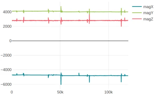
Each 2 minutes record contains 3-axis magnetic field data with the timestamp in millisecond started from 0 to 120,000. One of the magnetic field records can be seen in Figure 3.3. In the Figure, blue, green and red lines are the magnetic field record-ings of x, y, and z-axis respectively. The horizontal axis of the figure corresponds to the time in millisecond. Passing vehicles effect can clearly be seen from the figure.

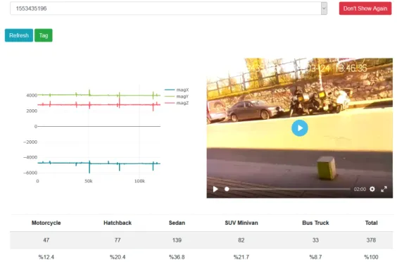
In the user interface, there is an option box which has a list of raw dataset recordings. By default, the first recording selected. On the left side, there is an interactive graph

(23)

of sensor readings for x, y, z-axis. On the right side, the captured video player is placed. Figure 3.4 shows the home screen of the user interface.

On the graph, you can able to select any range using the mouse and left click. You can start any place on the graph with a left mouse click and drag the mouse to determine where you want to stop. After this selection, the video will jump to the selected starting time. Moreover, there is no need to watch the whole video or synchronizing the video with sensor recording. Each time you select a range from the graph, the video jumps the selected range.

However, determining the endpoint of the vehicle signature is not clear. After you fit the waveform of vehicle signature on the graph, click the Tag button to label that vehicle selecting its label. When you submit, the sensor values in the selected range will be copied onto another csv file with its label. Then you can double click on the graph to turn it default view. Then you can continue with the next vehicle. Same process here, select the range and then submit it with a class label. Each time you submit, the statistics on the bottom of the page will be updated.

(24)

Figure 3.5 Dataset Label UI Marked Page

After you tag all vehicles in that raw dataset (1553435196 in Figure 3.4), you need to click ‘Don’t Show Again’ button. This will remove that raw dataset from the list. It is important to notice that, you may tag the same interval several times and each Tag request will create new vehicle data. This control belongs to the user. Tag each vehicle passing once, after completing the all passing, remove that dataset from the raw dataset. Then you can continue with the next raw recordings.

There are a couple of steps to label vehicles. First, it is required to extract the signature of each vehicle from raw recordings. For each vehicle signature, we will have a csv file that contains only vehicles magnetic field recordings. These csv files called marked dataset. In Marked page, the extracted vehicle dataset and their labels are shown. Figure 3.5 shows the marked page. The waveforms of vehicle signature can be seen one by one. Marked Download button on top of the page creates a zip file that includes all vehicle signatures. All labelled vehicle signatures on a separate csv file and one summary.csv file are in the zip. The summary file is Nx2 array (N labelled vehicle count, 374 on example). First column stores the filename for each vehicle sensor data, and second column stores their class names. The first ten rows of the summary file are shown in 3.1.

(25)

1664d7a5 − 369c − 46f f − a7be − 43d0587d5308, hatchback 55b1f ee5 − 9900 − 4112 − 960a − 61c2da9e7849, sedan 674718aa − 240b − 4b74 − af 8f − 7ba38eef 157a, truck aa485c94 − f adb − 4b45 − 9772 − 656b4c071433, hatchback 258abef 1 − f 776 − 4ce5 − bba0 − 1340857792e3, hatchback b8d2bb20 − f 897 − 48ed − a132 − 78f 82c7daac0, hatchback 41a4dab5 − 21f 9 − 4e0a − 992d − 7346be8c8669, suv 05e9f 1c6 − a1e2 − 45f a − baf c − 6136a077dc29, suv f e532f 8a − c335 − 45f 9 − a450 − 608c7f 84d73e, hatchback 92cf d54f − 9c39 − 4ad1 − 957f − d53891904b86, sedan

(3.1)

For example, a hatchback vehicle stored in 1664d7a5-369c-46ff-a7be-43d0587d5308 file. There is a file with the same name (UUID) in downloaded zip. These files contain 7 columns each, different number of rows regarding the length of vehicle transition. (All vehicles does not have the same length, speed, etc.). Here are the first ten lines of the hatchback file given in 3.2.

(26)

xRaw, yRaw, zRaw, xZero, yZero, zZero, time −4434, 3595, 2823, −30.5, −7.25, −4.25, 0 −4432, 3592, 2804, −28.5, −10.25, −23.25, 10 −4437, 3591, 2801, −33.5, −11.25, −26.25, 28 −4446, 3588, 2792, −42.5, −14.25, −35.25, 38 −4462, 3573, 2789, −58.5, −29.25, −38.25, 48 −4489, 3541, 2801, −85.5, −61.25, −26.25, 58 −4511, 3492, 2815, −107.5, −110.25, −12.25, 75 −4537, 3447, 2826, −133.5, −155.25, −1.25, 85 −4508, 3389, 2753, −104.5, −213.25, −74.25, 95 −4279, 3296, 2580, 124.5, −306.25, −247.25, 105 (3.2)

The page is shown in Figure 3.6, has the following purpose; it is not easy to select the starting and ending point of the vehicle passing in the first tagging step. Since this page shows only selected range, we could make it better (trimming from start and end). Therefore, it can be trimmed here. Again, you need to select a range using a mouse on the graph, then simply you click the ‘Trim’ button. Unlike tagging on the first step, since we want to improve already tagged recordings, each Trim request will overwrite the old one. Therefore, you can Trim a record as many times as you want. You can download the trimmed dataset by clicking the ‘Trimmed Download’ link on top.

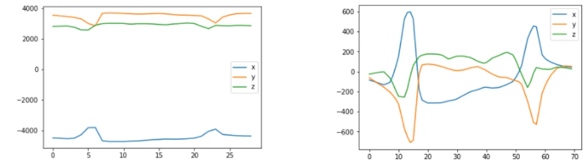
Finally, you can see the waveform of each vehicle using ‘Trimmed’ page. Figure 3.7 shows the record of one hatchback vehicle. On the left-hand side, you can see the original recordings (with earth magnetic field) and on the right-hand side, you can see the effect of the vehicle only (earth magnetic field removed). 3 axis of magnetometer values oscillate around zero.

(27)

Figure 3.6 Dataset Label UI Crop Page

Figure 3.7 Dataset Label UI Trim Page

Sedan, SUV-Minivan, and Truck-Bus. The distribution of vehicle signatures among classes can be seen in Figure 3.8.

(28)

3.2 Data Preprocessing

Since the speed and length of vehicles differ, the size of vehicle signatures measured also differ. The average length of 376 vehicles is nearly 70 discrete magnetic field recording. Therefore, all vehicle signatures lengths are equalized to 70 time frames using famous Python library numpy’s interpolation method.

After that, the Earth’s magnetic field is removed from each vehicle signature record-ings. Earth magnetic field for each axis calculated by taking the average of sensor readings while there is no passing vehicle nearby. Then for each vehicle signature recording, calculated average values are subtracted. Example of the labelled vehicle signature before the Earth’s magnetic field removed and after can be seen in Figure 3.9 and 3.10.

3.3 Outlier Analysis

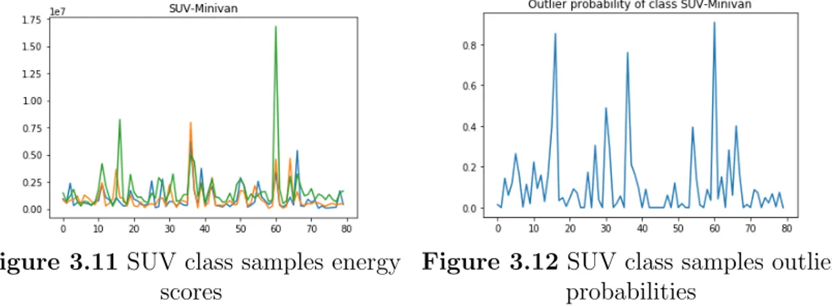
376 vehicle signatures inspected one by one and some of the vehicle signatures were noticed to have extreme magnetic field values. These anomalies are mostly caused by the error of magnetic sensor readings. In order to show these anomalies, 3 energy values for each magnetic axis of each vehicle signatures are calculated using equation 3.3.

Figure 3.9 Vehicle signature with Earth magnetic field

Figure 3.10 Vehicle signature without Earth magnetic field

(29)

energy[Xi] = 70 X j=1 (xij)2 energy[Yi] = 70 X j=1 (yij)2 energy[Zi] = 70 X j=1 (zij)2 (3.3)

Python’s PyNomaly library is used to carry out the outlier analysis over 3 features. PyNomaly implements the novel LoOP (Local Outlier Probability) outlier detection model that combines the idea of local, density-based outlier scoring with a prob-abilistic, statistically-oriented approach. Unlike the state-of-the-art unsupervised anomaly detection approaches, LoOP provides an outlier probability as score that is standardized, interpretable and can be compared over one data set and even over different data sets in [0-1] range. Using the calculated energy scores for each mag-netic field axis, LoOP probabilities are calculated. We ran LoOP for each class separately. A threshold of 0.5 is applied to eliminate the outliers, i.e., the observa-tions with LoOP probability > 0.5 are eliminated. Calculated energy scores for each samples in SUV class and their corresponding outlier probabilities shown in Figure 3.11 and 3.12.

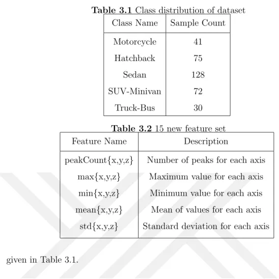
Regarding the outlier probabilities, 30 vehicle signatures are eliminated from 376 vehicle signatures. Remaining 346 vehicle signatures, each having 70 magnetic field values for each x, y, z axis are called Dataset I. The class distribution of samples are

Figure 3.11 SUV class samples energy scores

Figure 3.12 SUV class samples outlier probabilities

(30)

Table 3.1 Class distribution of dataset Class Name Sample Count

Motorcycle 41

Hatchback 75

Sedan 128

SUV-Minivan 72

Truck-Bus 30

Table 3.2 15 new feature set

Feature Name Description

peakCount{x,y,z} Number of peaks for each axis max{x,y,z} Maximum value for each axis

min{x,y,z} Minimum value for each axis mean{x,y,z} Mean of values for each axis

std{x,y,z} Standard deviation for each axis

given in Table 3.1.

Using this dataset, a second dataset is created. Fifteen new features are calculated from the Dataset I. Table 3.2 shows these fifteen features and their mathematical explanations.

3.4 Data Normalization

Before training of Neural Networks, normalization is applied to both datasets. There are several different effective methods in the literature. Min-Max scaler is found to be ineffective for time series magnetic field sensor data normalization. Almost all trained neural networks predict that all test samples as Sedan which has the majority in the datasets. Then using the equation 3.4, Mean-Std standardization is applied and better results are obtained.

(31)

xij = (xij− µ(Xi))/σ(Xi)

yij = (yij − µ(Yi))/σ(Yi)

zij = (zij − µ(Zi))/σ(Zi)

(32)

4. EXPERIMENTS

After creating the Dataset I and Dataset II, simple neural network and several different machine learning algorithms for multi class classification are trained.

4.1 Neural Network

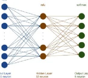
The Python Deep Learning library Keras is used to train the neural networks. Ini-tially, several well-known classifiers such as XGBoost, AdaBoost, BalancedRandom-ForestClassifier, and EasyEnsembleClassifier are tested. However, manually built Keras Neural Networks gave better initial results for both Dataset I and II. In Figure 4.1, basic properties of Neural Network that trained for first dataset are visualized. Same Network with 15 neuron in the first layer is used for the second dataset.

Using Grid Search 1008 different Neural Network (NN) trained for both Datasets I and II. Table 4.1 lists the parameters and exhausted values. Neuron count of hidden layers chosen to be 32, which is a popular value in network applications. Learning

(33)

Table 4.1 Grid Search Parameters

Parameter Name Tested Values

Activation Function relu, elu, sigmoid, tanh, exponential and hardsigmoid

Optimizer Function SGD, Adam, Nadam,

RMSprop, Adagrad, Adadelta and Adamax

Hidden Layer Count 0 and 1

Epoch 5, 20 and 50

Dropout 0, 20%, 50% and 80%

parameters and some other hyper-parameters of NN left as default values which performed better. For each network, the dataset is split into two parts, 30% for testing, 70% for training.

Activation functions are one of the fundamental parameters for Neural Networks. Activation functions make the NN learn a non-linear and complicated mapping between input and output variables. The weighted sum for each neuron is calculated using equation 4.1. The value of Y (the output) can be between minus and positive infinity. Activation function decides if the neuron will be activated or not. One of the most popular activation functions, ReLU is shown in Figure 4.2.

Y =X(weight ∗ input) + bias (4.1)

(34)

Another important function of Neural Networks is the optimization function. Since the main objective of learning is to reduce the difference between actual output and predicted output which is called cost or loss. The goal of the optimizer function is to update weight parameters to minimize loss. Categorical Cross-entropy function is used as the loss function during the experiments. During Grid Search 7 different optimizer functions had been applied to train the networks.

The hidden layers used in Neural Networks are to make them transform the previous layer to something else that improves the prediction. Since the dataset is small, more than one hidden layer deteriorated the accuracy. Therefore, two types of networks (no hidden layer and one hidden layer) have been trained.

While training the Neural Networks, one forward pass and one backward pass of all training samples count as one epoch. Initial tests showed that making the number of epochs more than 50 causes an over fitting problem. Therefore, 5, 20 and 50 epochs are tested for each network.

Dropout technique for over fitting problem is proposed by Srivastava et al. (2014). During the forward and backward weight updates, randomly selected neurons are ignored. Weights of neurons provide some specialization for specific features. And neighbours of neurons relies on this specialization and it makes network too special-ized in small datasets.

First layer, a.k.a. the input layer has the same number of neurons that the dataset feature count. For the first dataset, there are 70 magnetic field values for each axis, which equals 210 neurons. On the other hand, for the second dataset, there are fifteen neurons in the first layer. Last layer, a.k.a. the output layer has 5 neurons which are equal to the number of classes for both datasets. Since there are 5 classes, the softmax activation function used in the output layer.

Receiver Operating Characteristic (ROC) curves and Area Under the Curve (AUC) were proposed to evaluate networks’ performance (Hand & Till 2001). ROC is a

(35)

method for visualizing the performance of binary classifier while AUC is a num-ber that summarizes the performance of classifier between 0 and 1. In multi-class classification, the ROC method should be extended. For each class, one selected as positive and remaining classes joint together as negative. Then the ROC curve for each class plotted. Then 2 metrics, namely micro and macro average, calculated.

Precision values are calculated first for each class from the true positives (TP) and false positives (FP) using equation 4.2. Micro Average and Average for all networks calculated using equation 4.3 and 4.4 respectively.

precision = P RE = T P T P + F P (4.2) P REmicro = T P1+ ... + T P5 T P1+ ... + T P5+ F P1+ ... + F P5 (4.3) P REmacro= P RE1+ ... + P RE5 5 (4.4)

One of the example ROC AUC plot of trained networks can be seen in Figure 4.3. Classes 0, 1, 2, 3 and 4 correspond to Hatchback, Motorcycle, SUV-Minivan, Sedan, and Truck-Bus respectively. For that network, Micro average of ROC curve is 0.74 while Macro Average is 0.67.

(36)

4.2 Other Machine Learning Algorithms

Python Machine Learning library scikit-learn is used to train well-known classifi-cation algorithms on both datasets. 5-Fold Cross-validation with a random split is applied at each run and F1-Score and Cohen’s Kappa Score are saved for evaluation since the datasets are imbalanced.

F1-Score (a.k.a. f-score or f-measure) is commonly used in statistical analysis for classification problems. F1-Score measures the test’s accuracy considering both precision and recall of the test. In binary classification, F1-score is calculated using the equation 4.5. F1 score ranges between 0 and 1, which corresponds to the worst and the best results respectively. To extend the F1-score to a multi class problem, the same technique is applied to the AUC score.

F1 = 2 ∗

precision ∗ recall

(precision + recall) (4.5)

Cohen’s Kappa measure which measures inter-annotator agreement is also calculated for each run and saved. Cohen’s Kappa score equation is defined by J. Cohen as 4.6, where po is the empirical probability of agreement on the label assigned to

any sample, and pe is the expected agreement when both annotators assign labels

randomly (1960).

(37)

5. RESULTS

All obtained results are evaluated regarding the method and dataset that used. Experiments show that time series feature set (Dataset I) is better to train a Neural Network while the statistical feature set (Dataset II) is better for Machine Learning algorithms. However, the number of samples in the dataset clearly shows that the over fitting problem is inevitable while training the Neural Network. Oversampling and applying dropout technique were observed to be ineffective for our dataset.

5.1 Neural Network

Trained Neural Networks are evaluated using Area Under the Curve method. Micro and Macro AUC scores are calculated for each network and using these scores, different histograms are plotted. At first, the distribution of activation functions on micro and macro averaging is considered for each dataset. Then selecting the best activation function, other exhausted parameters’ effect are investigated.

Figures 5.1, 5.2, 5.3 and 5.4 shows the histogram of the AUC micro and AUC macro scores of activation functions for Dataset 1 and Dataset 2 respectively. For each dataset, exponential activation function causes the worst scores noticeably. Networks that used exponantial activation function mostly ended up with 0.5 AUC scores or worse. Therefore, it is not included in figures.

It is clear that the ReLU activation function outperforms other activation functions for the AUC metric for the first dataset. On the contrary, tanh function causes the worst predictions compared to others in the first dataset. Sigmoid and Hard Sigmoid activation functions have similar distribution for both scoring in the first dataset. While elu activation function has better scores sigmoid functions for AUC

(38)

Figure 5.1 Activation functions distribution on AUC Micro score in Dataset 1 macro metric, sigmoid functions have better scores for AUC micro.

On the other hand, elu activation function give comparable results with ReLU ac-tivation function in the second Dataset. Although its distribution is spread wider than ReLU, the best scores obtained with elu activation function are for AUC micro scores. However, remaining activation functions performed worse than elu and relu activation functions for the second dataset.

Having the ReLu activation function selected, the effect of optimizers plotted as a histogram for the first dataset. Figure 5.5 and 5.6 show the effect of the optimizer on AUC Micro and AUC Macro scores on first dataset respectively. seven different well-known optimizers are trained, Stochastic Gradient Descent optimizer for both Micro and Macro AUC scores has better scores than others with a small difference. In contrast, Adadelta optimizer has a worst distribution than other optimizers, again with a small difference. All activation functions have a similar effect on networks when the Dataset 1 is used.

The same approach is applied to the second dataset results, but elu activation func-tion is kept this time. Figure 5.7 and 5.8 shows the effect of optimizer on AUC Micro

(39)

Figure 5.2 Activation functions distribution on AUC Macro score in Dataset 1

Figure 5.3 Activation functions distribution on AUC Micro score in Dataset 2 and AUC Macro scores on the second dataset. In contrary to the first dataset re-sults, SGD optimizer gave worse results than other optimizers for the second dataset. However, distributions are very close to comparing optimizer functions on the second dataset. Still, Nadam optimizer is promising with a small difference.

(40)

Figure 5.4 Activation functions distribution on AUC Macro score in Dataset 2

Figure 5.5 Optimizer functions distribution on AUC Micro score in Dataset 1 dataset is used. Since the second dataset has non-linear features, hidden layers improve the accuracy. Even though the distributions of networks with or without hidden layer have similar results when the first dataset is used; still adding one hidden layer has a small positive effect. Effects of adding a hidden layer on AUC metrics for both datasets are shown in Figures 5.9 - 5.12.

(41)

Figure 5.6 Optimizer functions distribution on AUC Macro score in Dataset 1

Figure 5.7 Optimizer functions distribution on AUC Micro score in Dataset 2 Keeping ReLU activation function for the first dataset and elu for the second, dropout technique’s effect is shown in Figures 5.13 - 5.16. Employing the dropout technique improves the results if the first dataset is used. On the other hand, since there are only fifteen features in the second dataset, using a higher rate of dropout causes worse AUC scores since the big portion of the features were dropped.

(42)

Figure 5.8 Optimizer functions distribution on AUC Macro score in Dataset 2

Figure 5.9 Hidden Layer distribution over AUC Micro scores with first dataset Accuracy of the best performing network due to AUC micro averaging for the first dataset for 50 epochs training is plotted in Figure 5.17. ReLU activation function and SGD optimizer are used while training the network. Since the dataset is small, the over fitting problem occurs after 10 epoch of training. Similarly, Figure 5.18 shows the accuracy of AUC micro score for the second dataset where elu activation

(43)

Figure 5.10 Hidden Layer distribution over AUC Macro scores with first dataset

Figure 5.11 Hidden Layer distribution over AUC Micro scores with second dataset

function and Nadam optimizer are applied. Due to similar reasons, after fifteenth epoch, this network also shows an over fitting problem.

(44)

Figure 5.12 Hidden Layer distribution over AUC Macro scores with second dataset

Figure 5.13 Dropout distribution over AUC Micro scores with first dataset 5.2 Other Machine Learning Algorithms

Table 5.1 and 5.2 shows the result of all trained machine learning algorithms for the first and second dataset respectively. F1 and Cohen’s Kappa scores widely spread for both datasets as shown in figures.

(45)

Figure 5.14 Dropout distribution over AUC Macro scores with first dataset

Figure 5.15 Dropout distribution over AUC Micro scores with second dataset However, it is clear that the second dataset gave better Cohen’s Kappa scores com-pared to the first dataset. Even though the maximum F1 scores for both datasets are roughly the same, Cohen’s Kappa scores show that the second dataset is more suitable for machine learning algorithms.

(46)

ma-Figure 5.16 Dropout distribution over AUC Macro scores with second dataset

Figure 5.17 First Dataset, ReLu activation, SGD Optimizer accuracy graph of 50 epoch

Figure 5.18 Second Dataset, elu activation, Nadam Optimizer accuracy graph of 50 epoch

(47)

Table 5.1 Dataset I - ML Algorithm Results

Classifier F1-Score Cohen Cappa’s Score

SVC 0.492754 0.27521 GaussianNB 0.42029 0.252438 DecisionTreeClassifier 0.42029 0.219898 GradientBoostingClassifier 0.42029 0.207352 XGBClassifier 0.434783 0.205257 RandomForestClassifier 0.42029 0.201851 KNeighborsClassifier 0.318841 0.151491 MLPClassifier 0.347826 0.151176 AdaBoostClassifier 0.26087 0.098617 LinearSVC 0.275362 0.092583 RidgeClassifier 0.289855 0.073191 LogisticRegression 0.246377 0.049285 ExtraTreeClassifier 0.289855 0.044915 LinearDiscriminantAnalysis 0.188406 0.02621 QuadraticDiscriminantAnalysis 0.217391 -0.071922

chine learning classifiers for the second dataset. Likely, the second best Cohen’s Kappa score obtained by Gaussian Naive Bayes classifier for the first dataset. Fig-ure 5.19 and 5.20 show the confusion matrices of Gaussian NB classifier applied to first and second dataset.

Although the classifier demonstrated perfect accuracy with motorcycles, it per-formed poorly predicting trucks. These results are the effect of imbalanced dataset and shortage of samples. Generating artificial data using Synthetic Minority Over-sampling Technique as proposed by Chawla et al. (2002). Besides, Adaptive Syn-thetic methods also have proven to be effective (He et al. 2008). Both proposed technique applied to our datasets to improve accuracy. However, these techniques weren’t sufficient to improve the performance of trained machine learning algorithms in our case.

(48)

Table 5.2 Dataset II - ML Algorithm Results

Classifier F1-Score Cohen Cappa’s Score

GaussianNB 0.507246 0.369863 KNeighborsClassifier 0.492754 0.328234 QuadraticDiscriminantAnalysis 0.492754 0.324853 XGBClassifier 0.507246 0.318221 GradientBoostingClassifier 0.492754 0.296738 XGBRegressor 0.449275 0.283802 MLPClassifier 0.478261 0.278117 LinearSVC 0.478261 0.25895 RidgeClassifier 0.478261 0.244296 SVC 0.449275 0.213793 RandomForestClassifier 0.42029 0.19674 LinearDiscriminantAnalysis 0.42029 0.187758 DecisionTreeClassifier 0.362319 0.154318 DecisionTreeClassifier 0.362319 0.154318 AdaBoostClassifier 0.333333 0.103643 ExtraTreeClassifier 0.304348 0.076666

(49)

(50)

6. CONCLUSIONS

In this research, two different datasets are created using the magnetic field record-ings of passing by vehicles. Features of the first dataset are time series magnetic field values of vehicles. Using these time series values, some statistical features are cal-culated for each sample and the second dataset is created. Then for both datasets, 1008 Simple Neural Network trained using the Grid Search method. Besides, well-known other machine learning classifiers are applied to both datasets. As expected, time series dataset is more suitable for NN algorithms while the second dataset is more appropriate for Machine Learning algorithms.

The ReLU activation function is shown to be better than other activation functions in time series dataset while the exponential and tanh activation functions performed poorly. Also, SGD and Nadam optimizers gave better scores with respect to other optimizers. However, due to the fact that the dataset is small and imbalanced, over fitting problem occurred. Although the dropout technique improved predictions of networks, the over fitting problem couldn’t be solved with the reported results.

Gaussian Naive Bayes classifier has better Cohen’s Kappa score among other clas-sifier algorithms. However, it is clear that the accuracy of the classifier is not satisfactory, especially for Trucks and Hatchbacks. Again, oversampling methods are used to reduce misclassification rates. However, the performance of classifiers didn’t increase in the reported results. Collecting more vehicle samples are expected to solve the over fitting problem in NN and misclassification in ML applications.

(51)

REFERENCES

Chawla, N.V. et al., 2002. SMOTE: Synthetic Minority Over-sampling Technique. Journal of Artificial Intelligence Research, 16, pp.321–357. Available at: http://dx.doi.org/10.1613/jair.953.

Cohen, J., 1960. A Coefficient of Agreement for Nominal Scales. Educational and Psychological Measurement, 20(1), pp.37–46. Available at:

http://dx.doi.org/10.1177/001316446002000104.

Gupte, S. et al., 2002. Detection and classification of vehicles. IEEE Transactions on Intelligent Transportation Systems, 3(1), pp.37–47. Available at:

http://dx.doi.org/10.1109/6979.994794.

Hand, D.J. & Till, R.J., 2001. 10.1023/A:1010920819831. Machine Learning, 45(2), pp.171–186. Available at:

http://link.springer.com/10.1023/A:1010920819831.

He, H. et al., 2008. ADASYN: Adaptive synthetic sampling approach for

imbalanced learning. 2008 IEEE International Joint Conference on Neural Networks (IEEE World Congress on Computational Intelligence). Available at: http://dx.doi.org/10.1109/ijcnn.2008.4633969.

He, Y., Du, Y. & Sun, L., 2012. Vehicle Classification Method Based on

Single-Point Magnetic Sensor. Procedia - Social and Behavioral Sciences, 43, pp.618–627. Available at: http://dx.doi.org/10.1016/j.sbspro.2012.04.135. Hussain, K.F. & Moussa, G.S., 2005. Automatic vehicle classification system using

range sensor. International Conference on Information Technology: Coding and Computing (ITCC’05) - Volume II. Available at:

http://dx.doi.org/10.1109/itcc.2005.96.

Jeng, S.-T. (cindy) & Ritchie, S.G., 2008. Real-Time Vehicle Classification Using Inductive Loop Signature Data. Transportation Research Record: Journal of the Transportation Research Board, 2086(1), pp.8–22. Available at:

http://dx.doi.org/10.3141/2086-02.

Kleyko, D. et al., 2015. Comparison of Machine Learning Techniques for Vehicle Classification Using Road Side Sensors. 2015 IEEE 18th International Conference on Intelligent Transportation Systems. Available at: http://dx.doi.org/10.1109/itsc.2015.100.

(52)

Microaccelerometer for Target Classification. IEEE Sensors Journal, 4(4), pp.519–524. Available at: http://dx.doi.org/10.1109/jsen.2004.830950. Markevicius, V. et al., 2016. Dynamic Vehicle Detection via the Use of Magnetic

Field Sensors. Sensors , 16(1). Available at: http://dx.doi.org/10.3390/s16010078.

Ma, W. et al., 2014. A Wireless Accelerometer-Based Automatic Vehicle Classification Prototype System. IEEE Transactions on Intelligent Transportation Systems, 15(1), pp.104–111. Available at:

http://dx.doi.org/10.1109/tits.2013.2273488.

Ng, E.-H., Tan, S.-L. & Guzman, J.G., 2009. Road traffic monitoring using a wireless vehicle sensor network. 2008 International Symposium on Intelligent Signal Processing and Communications Systems. Available at:

http://dx.doi.org/10.1109/ispacs.2009.4806673.

Srivastava, N. et al., 2014. Dropout: a simple way to prevent neural networks from overfitting. Journal of machine learning research: JMLR, 15(1),

pp.1929–1958.

Tafish, H., Balid, W. & Refai, H.H., 2016. Cost effective Vehicle Classification using a single wireless magnetometer. 2016 International Wireless

Communications and Mobile Computing Conference (IWCMC). Available at: http://dx.doi.org/10.1109/iwcmc.2016.7577056.

Xu, C. et al., 2017. Vehicle Classification under Different Feature Sets with a Single Anisotropic Magnetoresistive Sensor. IEICE Transactions on Fundamentals of Electronics, Communications and Computer Sciences, E100.A(2), pp.440–447. Available at:

http://dx.doi.org/10.1587/transfun.e100.a.440.

Xu, C. et al., 2018. Vehicle Classification Using an Imbalanced Dataset Based on a Single Magnetic Sensor. Sensors , 18(6). Available at:

http://dx.doi.org/10.3390/s18061690.

Yang, B. & Lei, Y., 2015. Vehicle Detection and Classification for Low-Speed Congested Traffic With Anisotropic Magnetoresistive Sensor. IEEE Sensors Journal, 15(2), pp.1132–1138. Available at:

(53)