Data decomposition techniques for parallel tree-based k-means clustering

(1)

i

DATA DECOMPOSITION TECHNIQUES FOR

PARALLEL TREE-BASED K-MEANS

CLUSTERING

A THESIS

SUBMITTED TO THE DEPARTMENT OF COMPUTER ENGINEERING AND THE INSTITUTE OF ENGINEERING AND SCIENCE

OF BILKENT UNIVERSITY

IN PARTIAL FULLFILLMENT OF THE REQUIREMENTS FOR THE DEGREE OF

MASTER OF SCIENCE

By

Cenk Şen

July, 2002

(2)

ii

I certify that I have read this thesis and that in my opinion it is fully adequate, in scope and in quality, as a thesis for the degree of Master of Science.

Asst. Prof. Dr. Attila Gürsoy (Advisor)

Assoc. Prof. Dr. Özgür Ulusoy

Asst. Prof. Dr. Uğur Güdükbay

Approved for the Institute of Engineering and Science:

Prof. Dr. Mehmet B. Baray

(3)

iii

ABSTRACT

DATA DECOMPOSITION TECHNIQUES FOR PARALLEL TREE-BASED K-MEANS

CLUSTERING

Cenk Şen

M.S. in Computer Engineering Supervisor: Assist. Prof. Dr. Attila Gürsoy

July, 2002

The main computation in the k-means clustering is distance calculations between cluster centroids and patterns. As the number of the patterns and the number of centroids increases, time needed to complete computations increased. This computational load requires

high performance computers and/or algorithmic improvements. The parallel tree-based k-means algorithm on distributed memory machines combines the algorithmic improvements

and high computation capacity of the parallel computers to deal with huge datasets. Its performance is affected by the data decomposition technique used. In this thesis, we presented novel data decomposition technique to improve the performance of the parallel tree-based k-means algorithm on distributed memory machines. Proposed tree-based decomposition techniques try to decrease the total number of the distance calculations by assigning processors compact subspaces. The compact subspace improves the performance of the pruning function of the tree-based k-means algorithm. We have implemented the algorithm and have conducted experiments on a PC cluster. Our experimental results demonstrated that the tree-based decomposition technique outperforms the random decomposition and stripwise decomposition techniques.

(4)

iv

ÖZET

AĞAÇ TABANLI PARALEL K-ORTALI GRUPLAMA İÇİN VERİ DAĞITIM

TEKNİKLERİ

Cenk Şen

Bilgisayar Mühendisliği, Yüksek Lisans Tez Yöneticisi: Yard. Doç. Dr. Attila Gürsoy

Temmuz, 2002

K-ortalõ gruplamada asõl olan hesaplama yükü veri vektörleri ile gruplarõn ortalarõ arasõndaki uzaklõk hesaplamalarõdõr. Veri vektörlerinin ve grup ortalarõnõn sayõlarõ arttõrõldõkça, hesaplamalarõ tamamlamak için gerekli olan zaman artar. Bu hesaplama yükü yüksek performanslõ bilgisayarlar ve/veya algoritmik gelişmeler gerektirir. Büyük veri kümelerini işlemek için dağõnõk hafõzalõ makinalardaki paralel ağaç tabanlõ k-ortalõ algoritmasõ algoritmik iyileştirmeler ile paralel bilgisayarlarõn yüksek hesaplama kapasitesini birleştirmiştir. Algoritmanõn performansõ veri dağõtõm tekniğinden etkilenmektedir. Bu tezde, dağõnõk hafõzalõ makinalardaki paralel ağaç tabanlõ k-ortalõ algortimasõnõn performansõnõ arttõracak yeni bir veri dağõtõm tekniği sunduk. Önerilen ağaç tabanlõ dağõtõm teknikleri işlemcilere sõkõşõk altalanlar vererek toplam uzaklõk hesaplamalarõnõn sayõsõnõ düşürmeyi amaçlamaktadõr. Sõkõşõk altalanlar ağaç tabanlõ k-ortalõ algoritmasõnõn budama fonksiyonunun performansõnõ arttõrmaktadõr. Algoritmanõn gerçekleştirilmesi ve performans deneyleri gruplandõrõlmõş kişisel bilgisayarlar üzerinde yapõlmõştõr. Deney sonuçlarõmõz ağaç tabanlõ dağõtõm tekniğinin karõşõk dağõtõm ve şeritvari dağõtõm tekniklerinden daha iyi performansõ olduğunu göstermiştir.

(5)

v

Acknowledgement

I would like to express my special thanks and gratitude to Asst. Prof. Dr. Attila Gürsoy, from whom I have learned a lot, due to his supervision, suggestions, and support during the past year. I would like especially thank to him for his understanding and patience in the critical moments.

I am also indebted to Assoc. Prof. Dr. Özgür Ulusoy and Assist. Prof. Dr. Uğur Güdükbay for showing keen interest to the subject matter and accepting to read and review this thesis.

I would like to thank to my parents and my wife for their morale support and for many things.

I would like to thank to Turkish Armed Forces for giving this great opportunity.

I am grateful to all the honorable faculty members of the department, who actually played an important role in my life to reaching the place where I am here today.

I would like to individually thank all my colleagues and dear friends for their help and support.

(6)

vi

List of Figures

1.1 Stages in clustering……… 2

2.1 K-means clustering algorithm……… 9

2.2 The tree traverse function of the tree-based k-means algorithm……… 10

2.3 Example of the working of the pruning function while traversing the pattern tree.. 11

2.4 The pruning function of the tree-based k-means algorithm………... 13

2.5 The example for the pruning of the candidate cluster centroids……… 14

2.6 Parallel direct k-means clustering algorithm……… 16

2.7 Parallel tree-based k-means clustering algorithm………... 17

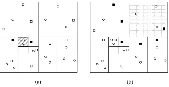
2.8 (a) The example of the effect of the compact subspace to the tree-based k-means algorithm.(b) The quadtree of the subspace………. 19

2.9 (a) The example of the effect of the larger subspace to the tree-based k-means algorithm. (b) The corresponding quadtree of the subspace……… 20

3.1 The effect of the size of the assigned subspaces: (a) the smaller subspaces. (b) the larger subspace………... 24

3.2 Strip decomposition of patterns………. 26

3.3 A two-dimensional pattern distribution and the corresponding quadtree………….. 28

3.4 Pattern tree partitioning scheme………. 29

3.5 The hierarchical representation (a) of the physical distribution of the patterns (b)... 30

3.6 The pruning rate of the two different cells, each of which has different heights….. 31

3.7 Tree decomposition with uniform numbered children………...35

3.8 100.000 patterns are distributed among 16 processors by uniform numbering of cells. Some of the subspaces are not contiguous………. 36

3.9 Ordering scheme of cells………37

3.10 Tree decomposition with non-uniform numbered children………38

3.11 100,000 patterns are distributed among 16 processors by using non-uniform numbering of cells………..39

4.1 Total execution times for all of the pattern decomposition techniques for DS11 data set…...……… 44

(9)

ix

4.2 The comparison chart of the execution times of the tree-based decomposition

techniques with different cost function……….. 45 4.3 The comparison chart of the execution times of the decomposition techniques for

DS15 data set.…...…...……….. 47 4.4 The comparison chart of the execution times of the decomposition techniques for

DS110 data set...……… 47 4.5 The comparison chart of the execution times of the decomposition techniques for

DS21 data set...……….. 50 4.6 The comparison chart of the execution times of the decomposition techniques for

DS21 dataset..……… 50 4.7 The comparison chart of the total number of the distance calculations for DS11 data

set.……….. 52 4.8 The comparison chart of the total number of the distance calculations for DS15 data

set…….……….. 54 4.9 The comparision chart of the total number of the distance calculations for DS110 data

set... 54 4.10 The comparison chart of the total number of the distance calculations for DS21 data

set ... 56 4.11 The comparison chart of the total number of the distance calculations for DS41 data

set... 56 4.12 The comparison chart of the speedup values of five decomposition techniques for

DS11 data set... 59 4.13 The comparison chart of the speedup values of five decomposition techniques for

DS110 data set... 60 4.14 The comparison chart of the speedup values of five decomposition techniques for

DS41 data set... 61 4.15 The load imbalance values caused by all decomposition techniques for DS110 data

set... 63 4.16 The comparison chart of the execution times of the decomposition techniques for

three data sets each of which has different number of patterns... 66 4.17 Comparison of the execution times of the decomposition techniques for three data sets

each of which has different number of clusters... 67 4.18 The comparison chart of the total distance calculations of the decomposition

(10)

x

4.19 The comparison chart of the total distance calculations of the decomposition

techniques for data sets DS11, DS21 and DS41... 70 4.20 The comparison chart of the speedup values of four decomposition technique for data

sets DS11, DS15 and DS110... 71 4.21 The comparison chart of the load imbalance of four methods as the number of the

(11)

xi

List of Tables

4.1 Properties of the data sets... 41

4.2 Total execution times (in seconds) for the standart parallel k-means and tree-based parallel k-means with different pattern decomposition techniques and with different number of processor for DS11 data set... 44

4.3 Total execution times (in seconds) for different pattern decomposition techniques with different number of processor for DS15 data set... 46

4.6 Total execution times (in seconds) for different pattern decomposition techniques with different number of processor for DS41 data set ... 49

4.7 Total number of distance calculations for DS11 data set... 51

4.11 The speedup values of all decomposition techniques for DS11 data set... 58

4.12 The speedup values of all decomposition techniques for DS15 data set... 59

4.13 The speedup values of all decomposition techniques DS210 data set... 60

4.14 The load imbalance values caused by all decomposition techniques for DS11 data set... 62

4.16 The load imbalance values caused by all decomposition techniques. The input dataset is DS21... 64

(12)

xii

List of Symbols and Abbreviations

PC : personal computer

n : number of the input patterns k : number of the input cluster

p : number of the processors in the system Pi : ith pattern

fix : xth feature of the ith pattern d : dimension of the data Cj : jth cluster

cj : centroid of the jth cluster

O

: asymptotic big OH

Minmax : minimum of the maximum distances N : cell of the pattern tree

SCF : simple cost function LCF : level cost function CCF : centroid cost function

LCFC : centroid and level cost function

(13)

CHAPTER 1 INTRODUCTION

1.1 Overview

Recent times have seen an explosive growth in the availability of various kinds of data. It has resulted in an unprecedented opportunity to develop automated data driven techniques of extracting useful knowledge. Data mining, an important step in this process of knowledge discovery, consists of methods that discover interesting, non-trivial, and useful patterns hidden in the data [2]. The field of data mining builds upon the ideas from diverse fields such as machine learning, pattern recognition, statistics, database systems, and data visualization. But, techniques developed in these traditional disciplines are often unsuitable due to some unique characteristics of today's data-sets, such as their enormous sizes, high dimensionality and heterogeneity [1].

The clustering problem has been addressed in many contexts and by researchers in many disciplines such as data mining [7], statistical data analysis [8], compression [4], vector quantization; this reflects its broad appeal and usefulness as one of the steps in exploratory data analysis. However, clustering is a difficult problem combinatorially, and differences in assumptions and contexts in different communities have made the transfer of useful generic concepts and methodologies slow to occur [3].

(14)

CHAPTER 1. INTRODUCTION 2 Cluster analysis is the organization of a collection of patterns (usually represented as a point in a multidimensional space) into clusters based on similarity. Intuitively, patterns within the same cluster are more similar to each other than they are to a pattern belonging to a different cluster [3]. The clustering process tries to increase similarity between patterns of a particular cluster, and tries to decrease similarity between patterns of different clusters. Clustering has been formulated in various ways in the machine learning [9], pattern recognition [10], optimization [11], and statistics literature [8,12]. Clustering can be simply formalized as follows: Given the desired number of clusters k and a dataset of n points, and a distance based measurement function (e.g., the weighted total/average distance between pairs of points in clusters), we are asked to find a partition of the dataset that minimizes the value of the measurement function [4]. So, the typical pattern clustering activity includes the following steps [6], which are depicted in Figure1.1. The first step is the pattern representation, which refers to the number of classes, the number of available patterns, and the number, type, and scale of the features available to the clustering algorithm. Some of this information may not be controllable by the practitioner. The second step is the definition of a pattern proximity measure appropriate to the data domain. It is the process of identifying the most effective subset of the original features to use in clustering. Pattern proximity is usually measured by a distance function, such as Euclidean distance, defined on pairs of patterns. The third step is clustering or grouping. This step can be performed in a number of ways so that there are many different clustering algorithms.

feedback loop Clusters Patterns Grouping/ Clustering Representations Pattern Feature Selection/ Extraction InterPattern Similarity

(15)

CHAPTER 1. INTRODUCTION 3 Since clustering is applicable to many different areas, variety of clustering techniques can be obtained. Categorization of these techniques according to their clustering structure shows that there are two major clustering algorithms, partitioning clustering and hierarchical clustering. In hierarchical clustering, each group of size greater than one is in turn composed of smaller groups. So, a hierarchical algorithm yields a dendrogram (tree) representing the nested grouping of patterns and similarity levels at which groupings change. In partitioning clustering every pattern is exactly in one group according to similarity measure. Partitional methods have advantages in applications involving large data sets for which the construction of a dendrogram is computationally expensive [3,13].

K-means is a partitional clustering method and because of its easy implementation it is one of the most commonly used clustering algorithm. The k-means method has been shown to be effective in producing good clustering results for many practical applications, for this reason there are variety of different implementations [15]. Inputs of the k-means algorithm are the patterns, the predefined number of clusters. Algorithm employs Euclidean distance based similarity metric function between center of predefined number of cluster and patterns. At each step, every pattern is assigned to the nearest cluster. After all patterns assigned, cluster centroids are updated to represent new clusters. These calculation operations are repeated until either no pattern need to be moved or predefined number of iteration of calculation process.

Most of the early cluster analysis algorithms come from the area of statistics and have been originally designed for relatively small data sets. In the recent years, clustering algorithms have been extended to efficiently work for knowledge discovery in large databases and some of them are able to deal with high-dimensional feature items. When they are used to classify large data sets, clustering algorithms become computationally demanding and require high performance machines to get results in reasonable time. Experiences of clustering algorithms taking from one week to about 20 days of computation time on sequential machines are not rare [16]. Thus, scalable parallel computers can provide the appropriate setting where to execute clustering algorithms for extracting knowledge from large-scale data repositories.

(16)

CHAPTER 1. INTRODUCTION 4 Over the last years parallel computing has received considerable attention of researchers in clustering. The main reason for the growing interest is the difficulties to increase performance of sequential computers due to technical and physical limitations. Also, the availability of cheap mass fabricated microprocessors and communication switches makes it more economical to connect hundreds of these components than to build highly specialized sequential computers. Such a collection of processors working in parallel can achieve unlimited performance and is suitable to solve problems of all areas of science.

The huge size of the available data-sets and their high-dimensionality make large-scale data mining applications computationally very intensive, because of its high-performance, parallel computing is becoming an essential component of the solution of the large scale data mining applications. Another opportunity that makes parallel computing popular in data mining is the quality of the data mining results. The quality of data mining results often depends directly on the amount of computing resources available, as the capability of computing resource is increased, the quality of the results are also increase. In fact, data mining applications will be the dominant consumers of supercomputing in the near future [18]. Although, designing parallel data mining algorithms is challenging, there is a necessity to develop effective parallel algorithms for various data mining techniques.

1.2 PROBLEM DEFINITION

In the k-means clustering, we have n patterns as an input each of which represents feature vector. Our main aim is to cluster n patterns to predefined number of clusters, denoted by k, with chosen similarity metric such as Euclidean distance.

The main computation in the k-means clustering is distance calculations between cluster centroids and patterns. As the number of the patterns and the number of centroids are increased, time needed to complete computations will be increased. It is clear that, execution time, per iteration of k-means, is sensitive to both the number of patterns and the number of centroids. Since today’s datasets are very huge, this computational load requires high performance computers and/or algorithmic improvements.

(17)

CHAPTER 1. INTRODUCTION 5 One of the new approaches to increase efficiency of the k-means algorithm is Alsabti’s tree-based k-means clustering with pruning some of the distance calculations [15]. In this approach, a pattern tree is built, each node of this tree contains a subset of patterns, as we traverse the pattern tree some candidate cluster centroids set is determined according to pruning algorithm. When only one candidate cluster is left, patterns, belonging to that tree node, are assigned to the cluster centroid without doing any distance calculation. This technique significantly decreases the execution time of the k-means clustering, by reducing the distance calculations.

Algorithmic improvements make k-means more efficient, however sequential k-means is still not satisfactory for really huge datasets. Parallelization may be one of the best choices for performance improvements of the k-means. The main workload of the k-means is the distance calculations between pattern and cluster centroids. One of the standpoints is that, calculations, made for each pattern, do not differ from pattern to pattern, k distance calculations are performed for each pattern. Besides, another standpoint of parallelization of k-means is that, the distance calculations are independent from each other. With these standpoints efficient parallelization of k-means can be accomplished by distributing equal number of patterns and a local copy of cluster centroids to each processor. Since computation load directly proportional to number of input pattern, each processor makes (n/p * k) calculations, where n is the total number of patterns, p is processor number, and k is number of cluster, per iteration. At the end of the distance computations, root processor makes update operation of the cluster centroids, and the new centroids are sent to the other processors for the next iteration. These steps are repeated until predefined condition is satisfied, such as predefined number of iteration, no pattern needs to be moved to new cluster. In the implementation of the direct parallel k-means, none of the parallelization issues, reference to parallel k-means such as load balancing, data locality becomes a problem.

Parallelization of the Alsabti’s tree based k-means method, for shared memory architectures, has been described in [2]. Parallel k-means clustering is more challenging because of the algorithm structure. Irregular tree decomposition of the space, which is directly related to the pattern distribution on the space, and changing computations due to the pruning algorithm, and also changing calculations during traversal of pattern tree, make parallelization of tree based k-means more challenging. Two different kinds of computations are done during traversal of the tree, leaf computations and non-leaf computations. In the leaf computations,

(18)

CHAPTER 1. INTRODUCTION 6 distances between the patterns and cluster centroids are measured and assigned to the nearest cluster. The amount of the leaf computation is directly related to the success of the pruning algorithm. Since the main computation load is proportional to the number of cluster centroids and the number of the patterns, more pruning in the candidate set of centroids and in the patterns, will ensure less leaf computations. So one of the problems is, to increase the candidate set of centroids pruning and to increase the number of pruned patterns, to decrease the leaf computations. In the non-leaf computations, candidate set is compared with the space covered by the node, and unrelated candidate clusters are pruned after these computations. Naturally, some of the candidate set of centroids might have been pruned in the upper level of the pattern tree; so, the number of non-leaf calculations can vary throughout internal nodes of the pattern tree.

Since data decomposition is very important issue for parallel tree-based k-means algorithm, we proposed a data decomposition technique, which decomposes patterns to processors in a manner that local patterns of the each processors is scattered in a smaller area. Thus, performance of the parallel tree-based k-means algorithm increases.

1.3. Outline of the Thesis

This work describes pattern decomposition techniques for parallel tree-based k-means algorithm on distributed system parallel computers with an experimental work on PC clusters. The data decomposition is very important issue for the parallel systems, because it affects the performance of the parallel algorithm. In this work we proposed tree-based pattern decomposition techniques, which improves the performance of the parallel tree-based k-means algorithm.

In the second chapter of the thesis, sequential standard k-means and sequential

tree-based k-means algorithms are explained in order to understand differences between

them. The parallelized version of the algorithms and their parallelizing issues are discussed. The importance of the pattern decomposition over the parallel tree-based k-means algorithm is presented.

(19)

CHAPTER 1. INTRODUCTION 7 In third chapter, proposed decomposition techniques and implementation details of them are described in details. Their standpoints are explained in details. The advantages and disadvantages of each of them are presented. In order to achieve better results, various cost functions, which are used to estimate computational load or leaf computations, are explained.

In the fourth chapter, the experimental results that are obtained by implementation of the algorithm on a PC cluster are reported. Each decomposition technique is examined with four metrics, all of these metrics are also overviewed. A comparison of the pattern decomposition technique is presented and the results of the experiments are analyzed. The results of the experiments are explained and supported with appropriate graphics.

(20)

CHAPTER 2 BACKGROUND

2.1 K-Means Clustering

The k-means clustering algorithm is the simplest and the most commonly used algorithm. It employs squared error similarity criteria, which is widely used criterion function in partitional clustering. It starts with predefined number of initial set of clusters and at each iteration, patterns are reassigned to the nearest cluster based on the distance based similarity measure, this process is repeated until a converge criterion is met such as no reassignment of any pattern to a new cluster or predefined error value. Let us examine k-means algorithm in detail.

Let say we have n input patterns and patterns are denoted by P1, P2, …,Pn. The pattern

Pi (ith pattern) consists of a tuple of describing features where features are denoted by fi1, fi2,

… , fid. A dimension represents each feature, where d is the number of dimensions of the value space. The second input of the algorithm is the predefined number of clusters, denoted by k. The number of the clusters cannot be changed during the execution of the algorithm. Let

C1, C2,…, Ck be the clusters, and each cluster is represented by its centroid. Let c1, c2, … ,ck be the centroids of the clusters. The sketch of the algorithm is illustrated in Figure 2.1. Algorithm works as follows: First, the initial cluster centroids are formed randomly. The distances between pattern Pi and all clusters are calculated and pattern Pi is assigned to the

(21)

CHAPTER 2. BACKGROUND 9

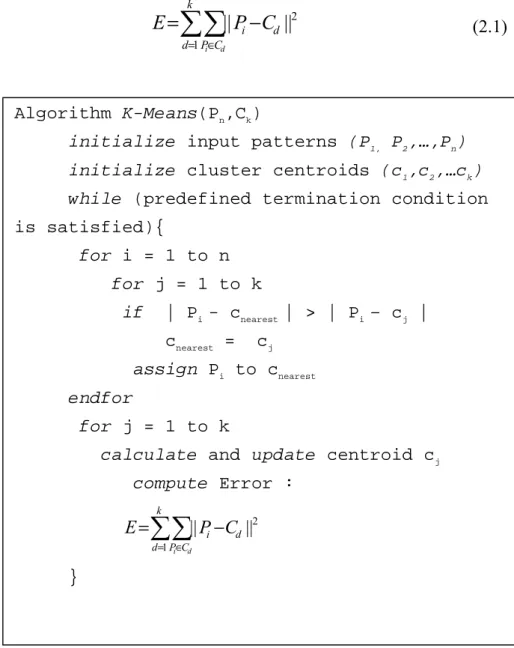
Figure 2.1: K-means clustering algorithm

Algorithm K-Means(P_n,C_k)

initialize input patterns (P_1, P₂,…,P_n)

initialize cluster centroids (c₁,c₂,…c_k)

while (predefined termination condition is satisfied){ for i = 1 to n for j = 1 to k if | P_i- c_nearest| > | P_i– c_j | c_nearest = c_j assign P_i to c_nearest endfor for j = 1 to k

calculate and update centroid c_j

compute Error :

∑∑

= ∈ − = k d PC d i d i C P E 1 2 || || }

closest cluster Cd. This process is repeated for all patterns and all patterns are assigned to a unique cluster. At the end of the iteration all centroids (c1,c2, … ,ck) are updated. In the next iteration, distance calculations between patterns and clusters are repeated with the updated centroids. The algorithm will iterate until predefined number of iteration is reached or no pattern is moved to new cluster. At the end of the algorithm, quality of the clustering is measured by the error function:

∑∑

= ∈

−

=

k d P C d i d i

C

P

E

1 2

||

_(2.1)

The time complexity of the direct k-meansalgorithm can de divided into three parts [15]. The time required for the assigning patterns to the closest cluster (first for loop in Figure 2.1) is O(nkd). The time required for updating the cluster centroids (second forloop in

(22)

CHAPTER 2. BACKGROUND 10 Figure 2.1) is O(nd). And the time required for calculating the error function is O(nd). Cleary, the computational cost of the algorithm is directly related to the number of the input patterns and the number of the input clusters. If these two input parameters are increased so much, direct implementation of the k-means can be computationally very expensive. This is especially true for today’s data mining applications with large number of pattern vectors.

There are some approaches described in the literature, which can be used to reduce the computational cost of the k-means clustering algorithm. One of the approaches uses the information from the previous iteration to reduce the number of the distance calculations. P-Cluster is a k-means based clustering algorithm, which exploits the fact that the change of the assignment of patterns to clusters are relatively few after the first few iterations [27]. It uses simple check that whether the closest cluster of a pattern has been changed or not. If the assignment has not been changed no further distance calculation is required for this pattern.

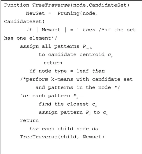
Function TreeTraverse(node,CandidateSet) NewSet = Pruning(node,

CandidateSet)

if | Newset | = 1 then /*ıf the set has one element*/

assign all patterns P_node

to candidate centroid c_c return

if node type = leaf then

/*perform k-means with candidate set and patterns in the node */

for each pattern P_i

find the closest c_c

assign pattern P_i to c_c return

for each child node do

TreeTraverse(child, Newset)

(23)

Alsabti et al. proposed another approach to reduce number of the distance calculations by pruning the cluster centroids and the patterns [15]. It uses a tree structure and organizes patterns with this structure, and then by using some geometrical constraints, it prunes some of the candidates. Even, when the candidate set of a pattern is consisting of only one cluster, it assigns pattern without any distance calculation, details of the algorithm will be given in the next section.

2.2 Tree-Based K-Means

Alsabti et al. proposed a tree-based k-means algorithm supported with pruning activity [15]. Their algorithm uses k-d tree structure to organize the input patterns according to their coordinates. The representation of the patterns provides rough grouping of patterns. Thus, patterns in a cell of the pattern tree are surely become closer to each other. The root of the pattern tree represents the all of the input patterns and covers all of the working space where is covered by the all input patterns. The children node of the pattern tree represents patterns in subspaces. 6 7 8 5 4 3 2 1

Figure2.3: Example of the working of the pruning function while traversing the pattern tree.

Square nodes represent inner nodes, circle nodes represent leaf nodes. The candidate clusters are written within the bracket.

1 _{{1,2,3,4,5,6,7,8}} 2 4 5 6 7 8 9 3 {3} {1} {1,2} {1,2,3,7} {2,3}

(24)

CHAPTER 2. BACKGROUND 12 In each iteration, the tree is traversed with depth first manner (Figure 2.2) as follows: The traverse of the tree is started at the root node, which has k candidate cluster centroids. At the each node of the pattern tree, the pruning function is applied to the candidate cluster set of the node. The pruning function will be explained in the next paragraph in detail. If the candidate cluster set has one cluster centroid, traversal of the tree is not pursued for the children of the node and all the patterns belonging to this node are assigned to the candidate cluster. Otherwise, traversal of the tree is pursued until the leaf node the pattern tree is reached. When a leaf node is reached, the pairwise distance calculations are performed between candidate cluster and patterns of the leaf node like in direct k-means, if the candidate set of clusters contains more than one candidate cluster. But the number of the calculations is possibly less than the calculations performed by the direct k-means, since pruning function eliminates some of the cluster centroids.

The example for the tree-based k-means algorithm is depicted in Figure 2.3. The quadtree of the input space is constructed. The square nodes represent inner nodes of the pattern tree and the circle nodes represent leaf nodes of the pattern tree. The number of the candidate cluster centroids is written near the nodes within a bracket. Initially, there are eight cluster centroids and all of them are candidate cluster for the root node, whose number is one. We started to traverse the tree from the root node and we apply the pruning function. The pruning function prunes different number of the candidate for the nodes so each children of the root node has different number of candidate set. For example, second node (first child of the root) has four candidate cluster centroids, while the fourth node (its second child). Then, the traversal of the tree continues with the second node, the pruning function is applied to the second node, and new candidate cluster set is constructed. Since new candidate cluster set has tree candidates, the standard k-means algorithm is applied between the candidate clusters and the patterns, which belong to second node. Unless, second node is leaf node, we would continue with applying pruning function to the first child of the second node. Then, the traversal of the pattern tree continues with the fourth node, which is second child of the second node. After the pruning function is applied to the seventh node, the candidate set of the seventh function has one candidate, thus all the patterns of the node are assigned to that candidate cluster and traversal of the tree does not pursue the children nodes of the seventh node. In other words, fifth, sixth and seventh nodes are assigned the candidate cluster number one without performing any distance calculation. Traversal of the tree continues with the eighth node. (third child of the second node). The candidate set of the eighth node has one

(25)

CHAPTER 2. BACKGROUND 13 element after the pruning function is applied. Although, eighth node is a leaf node, all the patterns belong to node will be assigned to the candidate cluster without performing any distance calculation. Traversal goes on top-down manner and traverses all of the nodes of the tree.

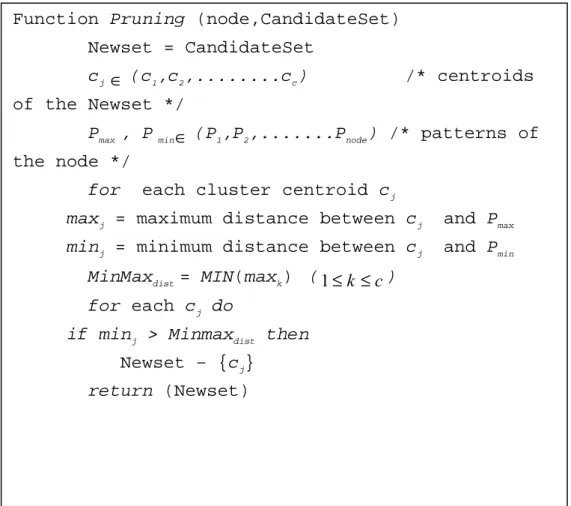
The improvements, which are achieved by the tree-based k-means are seriously rely on obtaining good pruning methods for obtaining less number of candidate cluster centroids for the next level. The pruning method used in Alsabti et.al. algorithm work as follows: For each candidate cluster centroids cd, the minimum and maximum distances are calculated to any pattern in the cell or subspace. Then determine the minimum distance of the maximum distances (MinMax) and eliminate any cluster centroids whose minimum distance is greater than the MinMax.

Function Pruning (node,CandidateSet) Newset = CandidateSet

c_j_∈ (c₁,c₂,...c_c) /* centroids

of the Newset */

P_max, P_min∈ (P₁,P₂,...P_node) /* patterns of

the node */

for each cluster centroid c_j

max_j = maximum distance between c_j and P_max min_j = minimum distance between c_j and P_min

MinMax_dist= MIN(max_k) (₁_≤_k _≤_c) for each c_j do

if min_j > Minmax_dist then

Newset – {c_j} return (Newset)

(26)

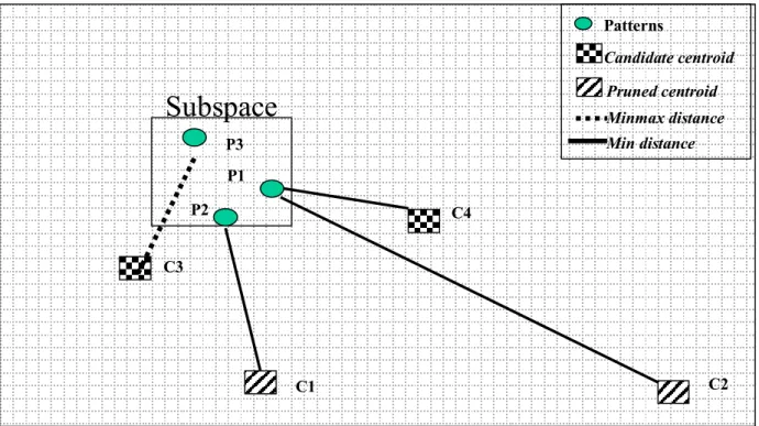
CHAPTER 2. BACKGROUND 14 To make Minmax clearer, the example of the pruning algorithm is given in Figure 2.5. Let say a node has a subspace in which there are three patterns and has a candidate set with four cluster centroids. In figure, the candidate clusters are represented by squares and circles represent the patterns. The pruning algorithm performs distance calculation between first candidate cluster and all patterns, then determine two distances; one of them is minimum distance between candidate cluster and any pattern in the subspace. The other is maximum distance between candidate cluster and any pattern in the subspace. For example minimum distance for cluster two is distance between cluster two and pattern one. The pruning algorithm finds minimum of the four maximum distances, calls it MinMax. In the example, centroid three has the minimum of the maximum distances. In the next step, algorithm compares the all of the minimums of the candidate clusters, if a cluster has a greater distance than the MinMax, algorithm prunes it. For example, centroid one and centroid two are pruned, because their minimum distances are greater than the MinMax. But, centroid four is not pruned since its minimum distance to any pattern in the subspace is less than the MinMax.

The pruning function requires distance calculations for the determination of the minimum and the maximum distances of the candidate clusters centroids to any pattern of the cell. Alsabti et al. have shown that maximum distance will be one of the corners of the cell.

P1 P3 P2 Patterns Candidate centroid Pruned centroid C3 C1 C2 C4 Minmax distance Min distance

Subspace

(27)

CHAPTER 2. BACKGROUND 15 Let the mostdistj be the furthest corner of the cell Ns for the cluster cj [15]. The coordinates of the mostdistj (mostdist1j, mostdist2j , . . . . , mostdistdj ) can be computed as follows:

if | l _jd | d c N − > | u _jd | d c N − mostdistjd = Ndl else mostdistjd = N_du where l d N and u d

N are the lower and upper coordinates of the cell along the dimension

d.

When the mostdistjd is determined we can compute the maximum distance of a candidate cluster as follows:

(

)

2

∑

−

= cjd mostdistjd

dist (2.2)

The value of the minimum distance of the candidate cluster is computed similarly. By using this approach, we do not have to calculate distances between candidate cluster centroids and patterns of the cell. Thus, this approach decreases the number of the distance calculations.

Alsabti et. al. mentioned that this pruning strategy guarantees that no candidate is pruned if it can potentially be closer than any other candidate prototype to a given subspace and the cost of pruning at a node is independent of the number of the patterns in the subspace and can be done efficiently. The results have shown that tree-based k-means is significantly faster than direct k-means. The reader is referred to [15] for the details.

In our implementation, we replaced k-d tree with tree-based quadtree. The quadtree is

a hierarchical data structure based on the principle of recursive decomposition of a space. The quadtree divides space into four equal-sized subspaces and each of which is represented as cells with same level. Each node of the tree has four children and contains the patterns falling in the region of that node. The details of the construction of the quadtree will be given in the next chapter.

(28)

2.3 Parallel Direct K-Means

The direct k-means has a problem associated that when the number of the input patterns and the number of the clusters are increased algorithm’s computational cost is increasing drastically. There are some approaches to decrease the number of the distance calculations in k-means, which are mentioned before. These approaches [15,27] are directly related with the algorithm of the k-means, they use some geometric constraints to decrease the number of the distance calculations. Another approach can be parallel implementation of the k-means algorithm.

In direct k-means algorithm, the main computation work is the distance calculations between patterns and the cluster centroids. It is clear that, for each pattern Pi, k distance calculations are performed. Since the predefined number of the cluster k, is fixed during the

iterations, the number of the distance calculations will not be changed from pattern to pattern. In addition he distance calculation between cluster and pattern does not change the location of the cluster for iteration, so that these distance calculation does not depend on each other, completely independent.

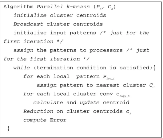
Algorithm Parallel k-means (P_n, C_k) initialize cluster centroids Broadcast cluster centroids

initialize input patterns /* just for the

first iteration */

assign the patterns to processors /* just

for the first iteration */

while (termination condition is satisfied){ for each local pattern P_{loc_i}

assign pattern to nearest cluster C_d

for each local cluster copy c_{copy_d} calculate and update centroid Reduction on cluster centroids c_k compute Error

}

(29)

CHAPTER 2. BACKGROUND 17 In the light of the above explanations, simple and the effective parallelization scheme would be as follows: Total number of the patterns is equally divided to processors in the system and a local copy of the cluster centroids are broadcasted, then each processor performs direct k-means algorithm with its local copy of the cluster and local patterns. Parallel k-means algorithm is sketched in Figure 2.6.

Parallelizing the direct k-means, for distributed memory machines is straightforward due to explained reason. In the parallel direct k-means, each processor is assigned to n/p

number of patterns, where n is the number of patterns and p is the number of the processors in

the system. The one of the processor, called root, broadcasts the cluster centroids to all

processors. At each iteration, processors perform single k-means iteration with their local copy of the clusters and their local patterns and update their local copy of the centroids. When the processor completes their computations, the root processor performs reduction for the

updated local copy of the cluster centroids of the processors, and updates the global centroids, which are the new cluster centroids set for the next iteration. This process continues until predefined termination condition is satisfied.

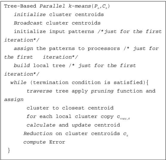
Tree-Based Parallel k-means(P_n,C_k) initialize cluster centroids Broadcast cluster centroids

initialize input patterns /*just for the first

iteration*/

assign the patterns to processors /* just for

the first iteration*/

build local tree /* just for the first

iteration*/

while (termination condition is satisfied){ traverse tree apply pruning function and

assign

cluster to closest centroid for each local cluster copy c_{copy_d} calculate and update centroid Reduction on cluster centroids c_k compute Error

}

(30)

CHAPTER 2. BACKGROUND 18 At this parallelization scheme, each processor has the same number of the patterns

(n/p) with a local copy of the cluster centroid. Thus each processor will perform the same

number of the distance calculation, which results with balanced computational load, so that one of the important problems of the parallelization is overcome by this parallelization scheme. This parallelization scheme will show almost linearly increasing speedup.

2.4. Parallel Tree-Based K-Means Clustering

The parallelization of the tree-based k-means can be a way to achieve better and faster clustering. But, it is not very straightforward because of the varying computational load balance. There is no so much difference between the parallel tree-based k-means and direct k-means. The most of the steps of the algorithms are same, just pruning function is added to the parallel direct k-means. The algorithm will be explained in details in the next paragraphs.

In parallel tree-based k-means, number of the patterns, assigned to the processors is determined by the pattern decomposition functions, which will be explained in the next section. Then, one of the processors; called root, broadcasts the local copy of the cluster

centroids to processors. The processors build their local pattern tree with their local patterns. While each processor is traversing its local pattern tree, it is also applying pruning function. This process continues until predefined termination condition is satisfied. When all of the processors finished their job, the root processor performs reduction of the updated local copy of the entire processors and updates global cluster centroids, which are the new centroid set of the next iteration. Figure 2.7 gives the parallel tree-based k-means algorithm.

When we compare the parallelization of the direct means and the tree-based k-means, we can easily obtain that parallelization of the tree-based k-means is more challenging because of the varying computational load. The tree-based algorithm performance is directly related with the performance of the pruning, since this pruning activity is changing according to some constraints such as size of the subspace, pattern density of the subspace etc., computational work load depends on the pruning activity is also varying from subspace to subspace.

(31)

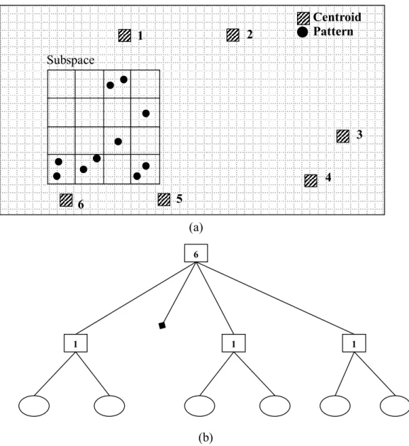
(b) (a)

The computations during traversal of the pattern tree can be divided into two groups [2]: the internal-node computations and the leaf-node computations. In the internal-node computations, computations for the pruning of the candidate clusters are done. Since some of the candidate cluster centroids might have been pruned upper levels of the pattern tree, the distance calculations can vary across the internal nodes. Similarly, as the number of the candidate set of the clusters and the number of the patterns are different in each cell, this results with difference in the number of the distance calculation and varying computational load. The leaf node computations are the distance calculations between patterns and candidate cluster centroids.

6

1 1 1

Figure 2.8: (a) The example of the effect of the compact subspace to the tree-based k-means

algorithm. Subspace is assigned to a processors. There will be more pruning at the upper level of the pattern tree.(b) The quatree of the subspace. The number of the candidate clusters is written inside the node

1 6 5 4 3 2 Centroid Pattern Subspace

(32)

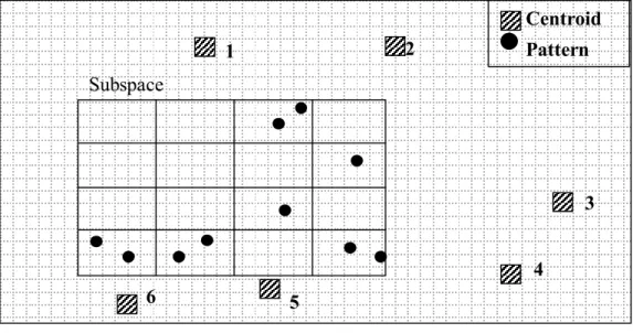
(b)

The tree-based k-means performance is directly related with the performance of the pruning algorithm like parallel version of the algorithm. When the number of the pruned candidate clusters and the patterns are increased performance of the algorithm also increases. Therefore, in order to increase the performance of the algorithm, pruning performance of the algorithm must be increased. For example, consider two processors with same number of patterns one with smaller subspace as shown in Figure 2.8 and another with larger subspace as shown in Figure 2.9. Figure 2.8-(b) represents the quadtree of the subspace, which is shown in the Figure 2.8-(a), and the number of candidate cluster centroids is written in the node

. 1 6 2 2 1 2 1 1 (a)

Figure 2.9: (a) The example of the effect of the larger subspace to the tree-based k-means

algorithm. The larger subspace is assigned to a processors. In this case there will be less pruning at the upper level of the pattern tree. (b) The corresponding quatree of the subspace. The number of the candidate clusters is written inside the node.

1 6 ₅ 4 3 2 Pattern Centroid Subspace

(33)

CHAPTER 2. BACKGROUND 21 The first processor starts traverse tree from the root node. The traversal of the tree continues with the first child of the root, when the pruning function is applied, five of the candidate clusters centroids (1,2,3,4,5) are pruned, because none of their minimum distances, between them and any pattern in the node are smaller than the Minmax distance. Thus, the

first child of the root node has the candidate set with a one element, and all of the patterns of the first child node will be assigned to sixth cluster centroid. The first processor continues to traverse tree with the third child. The pruning function is applied to candidate set of cluster, and the five of the six candidate cluster centroids (2,3,4,5,6) are pruned. Since, the third child’s candidate cluster set has one element, all of the patterns are assigned to cluster one.

Figure 2.9-(b) represents the quadtree of the larger subspace, which is shown in the Figure 2.9-(a). The second processor is assigned the larger subspaces shown in the Figure 2.9.a. It starts the traverse the tree, with the root node. Then it continues the traverse with first child of the root node. The pruning function is applied to the node and four of the six candidate cluster centroids( 1,2,3,4) are pruned. The traversal goes on with the first child of the first child, again the pruning function is applied and all the patterns are assigned to sixth cluster.

Then the next node is second child of the first child. After the pruning function is applied, two cluster centroids are left in the candidate set of the second child. Since the second child is the leaf node, the processor performs distance calculations between candidate clusters and the patterns of the node. The traversal of the tree goes on until the all nodes of the tree are visited. As we explained in the example the first processor who has smaller subspace performed less number of the distance calculations, most of the candidate cluster centroids are pruned at the first level of the tree. However, the second processor, which has same number of patterns but larger area, performed higher number of distance calculations, because most of the candidate clusters of it are not pruned at level one.

As a result, the more pruning of the candidate cluster centroids and patterns at the upper level of the pattern tree will result in the less distance calculations so that a processor with a smaller subspace will perform less number of distance calculation. In the case of larger subspace, the pruning performance is decreased, this will cause more distance calculations. In the light of the above explanations, if we assign compact subspaces to

(34)

CHAPTER 2. BACKGROUND 22 processors, the number of the distance calculations is decreased, and the performance of the parallel tree-based k-means is increased.

Pattern decomposition is important factor of increasing performance of the parallel tree-based k-means algorithm. To achieve better performance, pattern decomposition techniques must be handled very carefully, so we have examined and proposed new pattern decomposition technique. The decomposition techniques of the parallel tree-based k-means algorithms are explained in the next chapter.

(35)

CHAPTER 3

PATTERN DECOMPOSITION

Parallelizing tree-based k-means is not straightforward like standard k-means because of the parallelization scheme problems. The structure of the tree-based k-means is sensitive to load balancing. The pruning technique employed causes this sensitivity. Each processor’s pruning performance is varying according to its local patterns distribution. If patterns are distributed in a small space, there will be more pruning of candidate set of clusters at the upper levels of the tree, so leaf computations will be decreased. In the case of sparse distribution, there will be less pruning of candidate set of clusters at the upper levels of the tree, and then there will be more leaf computations than the small space distributed case. As a result, processor whose local patterns are distributed in a small space will have less computation load than the processor whose local patterns are sparse distributed (Figure 3.1).

In the light of the above explanations, we have implemented three different pattern decomposition techniques of parallel tree based k-means. These decomposition techniques are, random pattern decomposition, stripwise pattern decomposition and tree-based pattern

(36)

CHAPTER 3. PATTERN DECOMPOSITION 24

3.1 Random Pattern Decomposition

This decomposition technique is similar to technique used in parallel direct k-means. Each processor is assigned n/p local patterns; each of these patterns has been chosen randomly. It is

mostly probable that, local patterns of each processor are distributed in a sparse manner. This sparse distribution affects the performance of the pruning algorithm, in other words, performance of the tree-based k-means clustering algorithm.

Patterns are distributed among processors in the system as follows; The root processor randomly chooses n/p patterns for each processor without looking their location or without

paying attention whether they are distributed in a small space or not. The root processor only controls that pattern must be sent only one processor in the system. Then, root processor sends p pattern packed, each packed contains n/p patterns, to processors in the system.

Sparse distribution of the local patterns will cause less pruning of candidate set of Total space covered by all patterns

Cluster centroids

small subspace

Total space covered by all patterns

Cluster centroids

large subspace

(b) (a)

Figure 3.1: The effect of the size of the assigned subspaces: (a) The smaller subspaces. There

will be more pruning of candidate set of clusters centroids. (b) The larger subspaces. there will be less pruning of candidate set of cluster centroids, pruning will shift to leaves. Although, both processor have the same number of patterns (b) will do more calculations.

(37)

CHAPTER 3. PATTERN DECOMPOSITION 25 It is probable that every processor is assigned larger subspace, and many of the cluster centroids will be related with this subspace, so performance of the pruning algorithm will decrease. The pruning might shift towards to the leaves; this shifting might result in more distance calculation.

With this technique, we are expecting to have a balanced computational workload. Because, all of the processors have subspaces with almost equal sizes and have exactly same number of patterns. Also, random decomposition technique is easy to implement and it does

not need so much preprocessing work, which has done over the input pattern. However, each processor will have larger subspace (see Figure 3.1) so the pruning algorithm performs less pruning of candidate clusters at the upper level, and the number of the leaf computations will be increase, but it never reaches the number of the distance calculations performed by parallel direct k-means. The pruning advantage of the tree-based k-means is not used very much by

random pattern decomposition technique.

3.2 Stripwise Pattern Decomposition

If a processor is assigned to a compact subspace, we expect that, processor will perform better pruning activity, and the number of the leaf computations will decrease and then the performance of the algorithm will increase. So, we need a scheme that distributes more compact space to each processor.

Stripwise pattern decomposition technique distributes n/p patterns to each processor,

but each of n/p pattern set is belong to a more compact space when we compare with the random pattern decomposition. This set of patterns that are concentrated in small space,

ensures better pruning. Thus, the main goal of the tree-based parallel k-means algorithm is achieved.

In this technique, total space, covered by all patterns, is divided into the strips. All input patterns are sorted according to the one of the member of its feature vector space. The root processor divides sorted patterns to p strips each of which contains n/p patterns. These

strips are distributed to each processor. Each processor performs algorithm on these stripped set of patterns, which are concentrated on a small space.

(38)

CHAPTER 3. PATTERN DECOMPOSITION 26 We know that input patterns are distributed randomly. Their concentration is not uniform on the space, which is covered by all patterns, so that, pattern concentration of the stripes also is not uniform. This nonuniformity causes load imbalance. For example consider two processors, one with a pattern strip whose patterns are concentrated in a small space, and another one with a pattern strip, which has same number of patterns but patterns are less concentrated than the other. The first processor will prune many of the candidate cluster centroids at the upper level of the local tree. Because of the pruning algorithm specialty, some of the local patterns are assigned to a cluster without doing any distance calculation. Second processor will not prune many of the candidate cluster centroids, so number of the leaf computations will increase and the number of the tree-pruned patterns, which are assigned to a cluster without a leaf computation, is also increased. In other words, first processor will do less distance calculations than the second processor because first processor’s pattern strip is more compact than the other one.

In this decomposition technique we are expect to have less number of leaf computations, because stripwise decomposition will ensure better pruning. Since we will have less number of leaf computations and more tree pruned patterns, performance of the algorithm will be better than the algorithm whose assigned patterns are determined by the random pattern decomposition technique. But, the different concentration of the patterns on a strip will cause varying computations loads for each patterns.

Area covered by all patterns

P roces so r 2 P rocees or 1 P roces so r 3 P roces so r 4 P roces so r 5

Figure 3.2 : Strip decomposition of patterns . All processor have the same number of

(39)

CHAPTER 3. PATTERN DECOMPOSITION 27

3.3 Tree-Based Decomposition of the Patterns

The random decomposition technique and stripwise decomposition technique have

decomposed space, which is covered by all patterns, to subspaces by ignoring concentration of the patterns on these subspaces. They have just taken into account assigned number of patterns for each processor. They have tried to distribute equal number of patterns to each processor.

Size of the subspaces, assigned each processor, is determined by two factors. One of them is number of patterns assigned to each processor, and the other is concentration of patterns. Since each processor has equal number of patterns (n/p), the dominant factor in

determination of the size of the compact subspace is concentration of the patterns on that subspace. If the patterns are scattered in a small space, it means that the pattern concentration is high, it is clear that subspace will be compact. But the same number of patterns are scattered in a larger space then the subspace will invade larger area. The processor, whose subspace is highly concentrated, will perform more pruning, and less distance computations. But the other processor, whose subspace is not highly concentrated, will perform less pruning, and more distance calculations. In other words, the processor, whose subspace is compact area, will do less distance calculations than the processor whose subspace is larger. This situation is lead to load imbalance. This situation will be explained in detail in the next section.

To overcome load imbalance hierarchical representations of the physical space can be used. Tree structure is used for hierarchical representation of physical space, in most of the classical problems, such as n-body methods [23]. If we construct a pattern tree and then distribute this hierarchical tree structure, we are expecting to have improvements in the performance of the tree-based parallel k-means clustering algorithm.

In proposed decomposition technique, the input patterns are organized in a tree structure. We have already used the tree in tree-based k-means algorithm. The pattern tree is built by recursively subdividing space cells until predefined termination conditions, such as number of patterns per cell, are satisfied. In two-dimensional patterns, patterns are organized as quadtree structure [24], in which a subdivision divides cell area into four equal rectangular and each of cell has four children. In three-dimensional patterns, patterns are organized as

(40)

CHAPTER 3. PATTERN DECOMPOSITION 28 octree structure, whose cells have eight children and each subdivision operation divides cell into eight cubes.

Let us now describe the tree construction in some details. First of all, the positions of the patterns are used to determine the dimensions of the root cell of the tree. Then, tree is built by adding all patterns into the initially empty root. In our implementation, there are two termination conditions, predefined number of pattern per cell and predefined depth of the pattern tree. The root cell is controlled whether it is achieved to termination condition or not. If the root’s assigned number of patterns exceeds the predefined number of patterns per cell, then subdivision operation is started. The root cell is divided into four children (for the two-dimensional patterns, in case of three two-dimensional input children number will be eight.). Root cell’s patterns inserted into its children cell according to their location in the physical space. The subdivision operation is recursively applied to all children cell, until predefined termination condition is satisfied. In our implementation, depth of the tree is controlled at first, if this termination condition is satisfied then tree construction is terminated without controlling other termination condition. Otherwise, depth of the tree will be very high, which causes inefficient use of memory space and time. The result is a tree whose internal nodes are space cells and whose leaves are patterns. Because of the randomly scattered patterns, some of the cells might be empty, which are deleted. The tree is adaptive in that it extends to more levels in regions that have high pattern concentration. Figure 3.3 shows a small two-dimensional example domain and the corresponding quadtree.

(41)

CHAPTER 3. PATTERN DECOMPOSITION 29 After the pattern tree is built, next step will be partitioning the tree. This technique is very similar to costzones partitioning technique, which was discussed in the parallel n-body

implementations.[24]. We already have a hierarchical representation of spatial distribution of input patterns, so we will use this advantage by using costzones partitioning techniques.

Therefore, we will partition tree rather than partition the space and each processor is assigned to a smaller subspace. Partitioning procedure can be explained as follows: The root processor calculates the total cost of the domain with a chosen cost function by traversing the pattern tree. Each processor equally shares total cost in the system. After average cost for each processor is determined, which is equal to division of the total cost with the number of the processors in the system, the root processor distributes leaf cells of the tree. Patterns distribution policy is determined by the cost functions. Patterns may be distributed by either pattern-by-pattern or cell-by-cell. The leaf cell distribution of the pattern tree is lead to have each processor’s assigned patterns scattered to a compact space, which is our aim. The

costzones partitioning scheme is illustrated in Figure 3.4.

The main workload is directly proportional to the two factors, which are number of patterns and the number of cluster centroids. The predefined number of the cluster centroids is not varying throughout the clustering operation, so that, each input pattern has equal workload. The total workload is shared among processors by assigning different or equal number of patterns to each processor. Thus, cost functions, which are used to calculate total cost of the clustering operation, decides the number of patterns to be assigned for every

Figure 3.4 : Pattern tree partitioning scheme ([24]).

(42)

CHAPTER 3. PATTERN DECOMPOSITION 30 processor in the system. The cost functions will be explained in the following subsections in details.

3.3.1 Cost Functions

3.3.1.1 Simple Cost Function (SCF)

The simple cost function is straightforward. It assumes that, each pattern is associated with an equal workload in the each iteration of the algorithm. The input number of patterns is equal to total cost. The global average cost is calculated by dividing the total cost to number of the processor in the system. In other words, simple cost function assigns equal number of patterns to each processor. It can be formalized as follows:

tterns rofInputPa TotalNumbe TotalCost = ocessor numberofpr TotalCost t AverageCos = /

3.3.1.2 Level Cost Function (LCF)

Simple cost function depends on the assumption that, each pattern is associated with equal amount of work at the every iteration of the algorithm. However, tree-based parallel k-means algorithm performs cluster centroids pruning, and each pattern might have different amount of workload, even no workload, at the every iteration of the algorithm. So, there is a necessity for a cost function, in which the pruning specialty of the tree-based parallel k-means algorithm is not ignored.

(3.1) (3.2)

Figure 3.5 : The hierarchical representation (a) of the physical distribution of the patterns (b).

Patterns are represented by circles and centroids are represented by squares. As the depth of the tree increases, physical representatin of the nodes are getting smaller.