Cost-efficient approximation of linear systems with repeated and multi-channel filtering configurations

(1)

COST-EFFICIENT APPROXIMATION O F LINEAR SYSTEMS W I T H

REPEATED AND MULTI-CHANNEL FILTERING CONFIGURATIONS

M. A . Kutay,

M.

F. Erden,

H. M.

Ozaktas,

0. Arzkan,

c.

Candan, and

0. G.iilery.iiz

Bilkent University, Dept. of Electrical Engineering, TR-06533 Bilkent

,

Ankara, Turkey

ABSTRACT

It is possible to obtain either exact realizations or useful approximations of linear systems or matrk-vector products arising in many different applications, by synthesiz- ing them in the form of repeated or multi-channel filtering operations in fractional Fourier domains, resulting in much more efficient implementations with acceptable decreases in accuracy. By varying the number and configuration of filter blocks, which may take the form of arbitrary flow graphs, it is possible to trade off between accuracy and efficiency in the desired manner. The proposed scheme constitutes a systematic way of exploiting the information inherent in the regularity or structure of a given linear system or matrix, even when that structure is not readily apparent.

1. INTRODUCTION

Let f(u) denote the input and g ( u )

=

~ H ( u , U‘) f(u’) du‘ the output of an arbitrary linear system characterized by the kernel H ( u , U’). In some applications, such as image

enhancement, we may wish to implement a linear system deliberately designed to impart a certain effect on the input. In others, such as signal or image restoration or reconstruction, linear systems are used to recover a desired signal from whatever data or measurements are available. If we are working with signals whose time- or space-bandwidth products are NI the above may be approximated with the discrete form g k

=

cfit

Hkn f n ,

which is simply a matrix-vector multiplication of the form g

= Hf

This expression may either represent a matrix al- gebra operation we wish to implement or may constitute an approximation of its continuous counterpart. Digi- tal implementation of such general linear systems takes

O ( N 2 ) time. Common single-stage optical implementations, such as optical matrix-vector multiplier architectures or multi-facet architectures [l] require an optical system whose space-bandwidth product is O ( N 2 ) .

The output of a shift-invariant system characterized by the impulse response h ( u ) is related to the input by the relation g ( u )

=

J h ( u

-

u’)f(u’) d d whose discrete form is g k =

E

:

.

;

hk-,Jn, which is again a matrix- vector multiplication, but this time with the matrix being of a special form. Digital implementation of such shift-

invariant systems takes O ( N log N) time (by using the FFT). Optical implementation requires an optical system whose spacebandwidth product is O ( N ) .

Due to the intrinsic nature of some problems, convolution-type systems are fully adequate. However, in other cases, the use of shift-invariant systems is either totally inappropriate or at best a crude approximation which is employed only because of its significantly lower digital or optical implementation cost. This is not surprising given the fact that shift-invariant systems are a much more restrictive class than general linear systems, which is evident upon noting that general linear systems have N 2 degrees of freedom whereas shift-invariant systems have only N .

We may think of shift-invariant systems and general linear systems as representing two extremes in a cost- accuracy tradeoff. Sometimes use of shift-invariant systems may be inadequate, but at the same time use of general linear systems may be overkill and prohibitively costly. In such situations where both extremes are un- acceptable, or simply when we desire greater flexibility in trading off between cost and accuracy, it would be desirable to be able to interpolate between these two ex- tremes. There may be many ways of achieving this. In

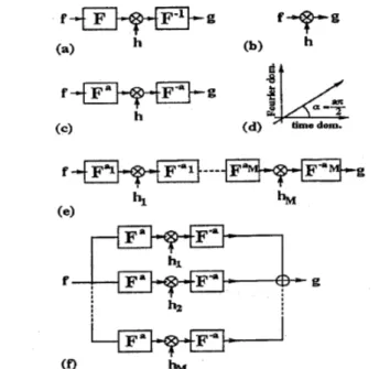
this paper we will consider repeated and multi-channel filtering in fractional Fourier domains. Common single- stage Fourier-domain filtering is shown in Fig.la. The dual of this operation is single-stage time-domain filtering, and is shown in Fig.lb. Fig.lc depicts single-stage filtering in the ath order fractional Fourier domain. This filtering configuration and its applications are discussed in [2, 31.

The uth order fractional Fourier transform of f(u) is

denoted by fa(.) and given by [4, 51

cn

ei*(COtCC Ua-2CSCCZ U U ‘ + C O t U U ‘ a ) f ( u I ) du’

fa(.) = A ,

J

I

-cn

(1) for a

#

2 j , and fa(.> = f ( u ) for a

=

4 j and fa((.)

=

f(-u) for a = 4 j f 2, where j is an integer, (Y

=

a ~ / 2 ,

and A ,

=

d-.

The 0th transform of f(u) is sim- ply fo(u) =

)

.

(

p

itself and the 1st transform is simply fl(u) = F ( u ) , the ordinary Fourier transform. The aath transform of the a l t h transform is equal to the (az+ui)th transform, a property known as index additivity. fa(.)

(2)

Figure 1: Single-stage filtering in the Fourier domain (a), the time domain (b), and the ath order fractional Fourier domain (c). ath order fractional Fourier domain (d). Re- peated (series) filtering (e). Multi-channel (parallel) filtering (f).

is also referred to as the representation of f(u) in the ath fractional Fourier domain. The ath fractional Fourier do- main makes an angle a

=

a7r/2 with the time (or space) domain in the time-frequency (or space-frequency) plane (Fig.ld) [4, 61. This is confirmed by the fact that the in-

tegral projection of the Wigner distribution of f(u) onto

-

this domain equals lfa(u)12.

2. R E P E A T E D A N D MULTI-CHANNEL FILTERING

In the repeated filtering scheme (Fig-le) first suggested in [7, 41, the input is first transformed into the a l t h domain where it is multiplied by a filter h l ( u ) . The result is then transformed back into the original domain. This process is repeated M times.l (The back transform of stage k with order a k , may be combined with the for- ward transform

of

stage

k

+

1 with order Q+I, resulting in a single transform of order ak+l

-

U k . Thus the system consists of multiplicative filters sandwiched between fractional transform stages of order a i = ak+l - a k . )

The multi-channel filter structure consists of M single- stage blocks in parallel. For each channel I C , the input is transformed to the akth domain, multiplied with a filter l I t has been shown in [SI that, by modifying the filters h, (U)

appropriately, the repeated configuration can be reduced to one involving only ordinary Fourier transforms. However, the modified filters often exhibit oscillatory behavior so that this reduction is not necessarily beneficial in practice.

3434

&(U), and then transformed back. (More generally, we

may choose not to back transform, or to transform to some other domain.)

Let hj, denote the nth sample of the j t h filter h j ( u ) , and Aj denote the diagonal matrix whose elements are equal to those of the vector hj

=

[hj, h j ,

.

h j N - l ] T . Then, the output vectors g are related to the input vectors f according to the relations2

g

=

[ F - a M A ~ .

.

.Fa2-"'AlFa1] f , ₍₂₎

g =

C F - ~ ~ A ~ F ~ ~

f , (3)

[ k I l

1

where F"j represents the discrete aj th order fractional Fourier transform matrix [9]. The above may also be expressed as g = Tf where T is the matrix representing the overall filtering configuration.

Both filtering configurations have at most M N

+

M

degrees of freedom. Their digital implementation will take O ( M N log N ) time since the fractional Fourier transform can be implemented in O ( N log N ) time [9]. Optical implementation will require an M-stage or M-channel optical system, each with space-bandwidth product N [lo]. We see that these configurations lie (interpolate) between general linear systems and shift-invariant systems both in terms of cost and flexibility. If we choose

M to be small, cost and flexibility are both low. If we choose M larger, cost and flexibiIity are both higher. In

between, these systems give us considerable freedom in trading off efficiency and flexibility for each other, the latter which will translate into a better approximation and greater accuracy in most applications.

M

= 1 corresponds to single-stage filtering. As

M

approaches N , the number of degrees of freedom of the repeated filtering configuration approaches that of a general linear system. The important point is that increasing M gives us greater flexibility and will allow us to realize a broader class of linear systems, or put in a different way, to better approximate a given linear system. In other words, the capabilities of an M-stage system can be characterized in two ways. First, for a given value of MI we can realize a certain subset of all linear systems ezactly (or to some other specified degree of accuracy). As M increases, the subset in question becomes larger and larger. Second, and perhaps more useful, is to consider the problem of approximating a given linear system. For a given value of M I we can approximate this system with a certain degree of accuracy (or error). For instance, a shift-invariant system can be realized with perfect accuracy with M

=

1.

In general, there will be a finite accuracy for each value of M . As M is increased, the accuracy will usually in- crease (but never decrease). Thus, in the context of a particular application or problem, we can seek the minimum value of M which results in the desired accuracy, 2The extension to two-dimensions and/or rectangular matrices is straightforward.

(3)

or the highest accuracy (or minimum error) that can be achieved for a given value of M . Of course, this amounts to seeking the best performance for given cost, or least cost for given performance. Such cost-performance points are referred to as Pareto optimal cost-performance com- binations. The locus of such Pareto optimal points constitutes the cost-performance tradeoff curve.

The proposed system can be used in a given application in one of two distinct ways, which we now distin- guish. (i) Starting with a signal restoration, recovery, or reconstruction problem, we determine the optimal linear estimation or reconstruction matrix using any models and methods considered appropriate. Or, we may simply be given a matrix H to multiply input vectors f with. Then, we seek the transform orders aj and filters hj such

that the resulting matrix T (as given by (2) or (3)) is as close

as

possible to

H

according to some specified criteria. (ii) We take (2) or (3) as a constraint on the form of the linear estimation or reconstruction matrix to be employed. Given a specific optimization criteria, such as minimum mean-square error, we find the optimal values of aj and_hi such that the given criteria is optimized.

3. EXAMPLES

The repeated filtering configuration has been taken up in

Ell, 12,131, where its usefulness is discussed at length and several application examples are given. We also compare the accuracies and costs obtained with direct exact implementation of general linear systems and with the best approximation possible with single-stage filtering systems. We give many examples where it is possible to obtain useful approximations by using only a moderate number of stages. The corresponding full-length treatment of the more recent work on the multi-channel configuration will be subsequently reported. Here we must satisfy ourselves with a few illustrative examples.

Our first example is the restoration of signals de- graded by space-variant atmospheric turbulence using the repeated filtering configuration. Using approach (i), the resulting normalized mean-square difference between

H and

T

is 11% with M

=

4 and

<

1% with

M

=

8.

Us-

ing approach (ii)

,

the resulting normalized mean-square error between the actual signal and its estimate is

<

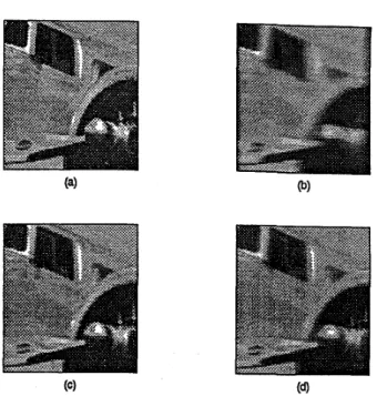
1% with M = 4.

In our second example, we consider restoration of im- ages blurred by a non-constant velocity (space-variant) moving camera. We use approach (ii). Fig.2 shows the results. The mean-square estimation error is 5% in the repeated case and 7% in the multi-channel case for M

=

5 , representing significant improvements with respect to

single-stage ( M = 1) filtering. Ordinary Fourier domain filtering gives very poor results. Although the errors obtained in both cases are close in this example, this is not always so. Often one or the other is clearly superior. Furthermore, repeated may be better for certain values

Figure 2: Original image (a). Blurred image (b). Re- stored by repeated filtering (c). Restored by multi- channel filtering (d).

of M and muIti-channel for the other values of

M.

Finally we consider the problem of recovering a signal corrupted with several additive chirp distortions. We assume that the second-order statistics of the signal and chirp distortions are given. In our example, we assume that the Q chirps have uniformly distributed random am- plitudes and time shifts, and their chirp rates are clus- tered around

P

(initially unknown) values. For Q

=

9,

P

=

3 the multi-channel configuration (approach (i)) re-

sults in a mean-square error

<

1% with

M

=

3.

We have employed an iterative algorithm to determine the optimal filters

hj

which minimize mean-square error. (The repeated system is highly nonlinear and does

not admit an exact solution. The multi-channel system is linear and has an exact solution, but in practice an iterative solution is preferred.)

In the last example we have optimized over the three orders 01, a2, as, whereas in the second example the orders were chosen to 'be equally spaced between 0 and

1. Whereas optimizing over the orders will always yield better results, this may be difficult when M is large. How to choose a set of orders a1,a2,

. . .

,

aM suitable for given application classes or with certain desirable properties is the subject of current research.

4. DISCUSSION AND CONCLUSION The repeated and multi-channel configurations may be based on other transforms with fast algorithms, instead of the fractional Fourier transform. For instance, the three- 3435

(4)

parameter family of linear canonical transforms may be used in place of the fractional Fourier transform. Con-

centrating on (3), the essential idea is to approximate a general linear operator a9 a linear combination of opera-

tors with fast algorithms. If an acceptable approximation can be found with a value of M which is not too large, the computational burden can be significantly reduced.

The singular value decomposition (SVD) of H leads to a similar approximation if we keep only the M largest sin- gular values and discard the others: g

=

[CEl

A k U k ] f .

Since

Uk

is of outer-product form, its implementation takes only O ( N ) time for an overall implementation time of O ( M N ) . For the chirp distortion example considered above, M

=

3 results in an error of 20%. Whereas (3)

gives good results for M

2 P,

the SVD approach gives comparable results only when M

2

Q. It is also possible to find many examples in which the SVD approach gives better results.

n

Figure 3: Each block corresponds to figure IC.

The series

and

parallel filtering configurations may be combined in arbitrary manner to give what we term gen-

eralized filtering configurations or circuits

(Fig.3).

What type of circuits may be beneficial in what circumstances is an area for future research.

Naturally, the number of stages and filters required to attain a given accuracy will be smaller for matrices ex- hibiting greater regularity or other more subtle forms of intrinsic structure. In such cases, direct implementation of the matrix-vector product is clearly inefficient. The regularity or structure inherent in a given matrix can be exploited on a case by case basis through ingenuity or

invention; most sparse matrix algorithms and fast transform algorithms are obtained in this manner. In contrast, ficient implementation which does not require ingenuity on a case by case basis. This approach would be espe- cially useful when the regularity or structure of the matrix is not simple or is not expressed symbolically or when we are presented with a specific matrix in numerical form

for which no easily discernible regularity or structure is apparent.

A distinct circumstance in which the method may be beneficial, even when a strong intrinsic structure does not exist, is when it is sufficient to compute the matrix-

our method provides a systematic w a y of obtaining an ef-

vector product with limited accuracy. This may be the case when some other component or stage of the overall system limits the accuracy to a lower value anyway, or simply when the application itself demands limited accuracy.

w e also expect the proposed filtering architectures to result in-possibly parallel and pipelined-efficient VLSI implement at ions.

5.

REFERENCES

[I] D. Mendlovic and H. M. Ozaktas. Optical-coordinate transformation methods and optical-interconnection ar- chitectures. Appl. Opt., 32:5119-5124, 1993.

[2] M. A. Kutay, H. M. Ozaktas, 0. Ankan, and L. Onural. Optimal filtering in fractional Fourier domains. IEEE

Trans. Sig. Proc., 45:1129-1143, 1997.

[3] M. F. Erden, H. M. Ozaktas, and D. Mendlovic. Synthe- sis of mutual intensity distributions using the fractional Fourier transform. Opt. Commun., 125:288-301, 1996. [4]

H.

M. Ozaktctas, B. Barshan, D. Mendloec, and L. Onu-

ral. Convolution, filtering, and multiplexing in fractional Fourier domains and their relation to chirp and wavelet transforms. J. Opt. Soc. Am. A

,

11:547-559, 1994.

[5] L.

B.

Almeida. The fractional Fourier transform and time-frequency representations. IEEE Trans. Sig. Proc.,

42:3084-3091, 1994.

[6] A. W. Lohmann. Image rotation, Wigner rotation, and the fractional order Fourier transform. J. Opt. Soc. Am. A, 10:2181-2186, 1993.

[7]

H. M.

Ozaktas snd D. Mendlovic. Fractional Fourier transforms and their optical implementation, 11. J. Opt.

Soc. Am. A 10:2522-2531, 1993.

[8]

H.

M. Ozaktas. Repeated fractional Fourier domain fil- tering is equivalent to repeated time and frequency domain filtering. Sig. Proc.

,

54:81-84, 1996.

[9]

H.

M. Ozaktas, 0. Ankan, M. A. Kutay, and G. Bozdagi. Digital computation of the fractional Fourier transform.

IEEE Trans. Sig. Proc., 44:2141-2150, 1996.

[lo]

H. M.

Ozaktas and D. Mendlovic. Fractional Fourier o p tics. J. Opt. Soc. Am. A , 12:743-751, 1995.

[ll] M. F. Erden. Repeated Filtering in Consecutive Frac- tional Fourier Domains. Ph.D. Thesis, Bilkent Univer- sity, Ankara, 1997.

[12] M. F. Erden, M. A. Kutay, and H. M. Ozaktas. Repeated filtering in consecutive fractional Fourier domains and its application to signal restoration. Sub. to IEEE Trans.

Sig. Proc.

1131 M. F. Erden, and H. M. Ozaktas. Synthesis of general linear systems with repeated filtering in consecutive frac- tional Fourier domains. Sub. to J. Opt. Soc. Am. A.