Animation of deformable models

A n i m at io n of d e f o r m a b I e

m o d e l s

U0ur G0d0kbay and B01ent OzgiJ9

present faster and simpler formulations to build and Although kinematic modelling methods are adequate for control the motions of models using physically based describing the shapes of static objects, they are insufficient when

it comes to producing realistic animation. Physically b a s e d appr°achest"

Another aspect in realistic animation is that of modelling remedies this problem by including forces, masses, modelling the behaviour of deformable objects. To strain energies and other physical quantities. The paper simulate the behaviour of deformable objects, we should describes a system for the animation of deformable models. The

system uses physically based modelling methods and approximate acontinuousmodel by usingdiscretization methods, such as finite difference methods and finite approaches from elasticity theory for animating the models, element methods. For finite difference discretization, a Two different formulations, namely the primal formulation and deformable object could be approximated by using a grid the hybrid formulation, are implemented so that the user can of control points where the points are allowed to move select the one most suitable for an animation depending on the in relation to one another. The manner in which the rigidity of the models. Collision of the models with impenetrable points are allowed to move determines the properties of obstacles and constraining ofthe model points to fixed positions the deformable object. Various researchers ~-s have in space are implemented for use in the animations, presented discrete models to define and enforce constraints for modelling and animating deformable

Keywords: modelling, animation, simulation

objects.

The plan of this paper is to first present a short description of the formulations which we have used to An animation system which is implemented for the animate elastically deformable models. We will then animation of nonrigid (deformable) models is discussed explain the implementation details of these formulations in this paper. The system is built on top of a modelling in the context of our system, and the algorithmic solution system for representing 3D freeform objects 1. The static of the problems, such as the collision of flexible models models obtained can be animated using the techniques with impenetrable obstacles. Then, some simulation discussed in this paper. The system is implemented using results representing the features of the system are given c language on a Unix* workstation environment (it runs and a quantitative comparison of the formulations is

on Sun 3 and Sparc workstations), presented. Finally, conclusions are given.

Currently, most of the methods used for modelling are kinematic. This becomes a major drawback when we want

to create realistic animation since these methods are N O N R I G I D M O D E L S passive; they do not interact with each other or with

external forces. The behaviour and forms of many objects To animate nonrigid objects in a simulated physical are determined by the objects' gross physical properties, environment, we should use the methods of elasticity To build and animate active models, physically based theory. Elasticity theory provides methods to construct techniques should be used. These techniques facilitate the the differential equations that model the behaviour of creation of models capable of automatically synthetizing nonrigid curves, surfaces, and solids as a function of time. complex shapes and realistic motions that are attainable Real materials exhibit both elastic and inelastic only by skilled animators. Physically based modeUino behaviour. Some materials undergo perfectly elastic achieves this by adding physical properties to the models, deformations so that, when the forces acting on the Such properties may be forces, torques, velocities, materials are removed, objects restore themselves to their accelerations, kinetic and potential energies, heat etc. natural shapes completely, However, there are other Physical simulation is then used to produce animation materials, such as cloth, paper etc., which restore on the basis of these properties. Researchers continue to themselves to their initial shapes slowly (or partially)

upon removal of the forces that cause deformations. *Unix is a registered trademark of AT&T Laboratories, USA. To model elastic materials, physical properties such as

tension and rigidity should be simulated. In this way, Department of Computer Engineering and Information Science, Bilkent

University, Bilkent, 06533 Ankara, Turkey fA complete bibliography of computer animation can be found in Paper received." 7 October 1993. Revised: 28 May 1994 Reference 2.

0010-448519411210868-08 © 1994 Butterworth-Heinemann Ltd 868 Computer-Aided Design Volume 26 Number 12 December 1994

Animation of deformable models: U G0d0kbay and B Ozg09 static shapes of a wide range of deformable objects, The distance between these points in the deformed body including string, rubber, cloth, paper, and flexible metals, in Euclidean 3-space is given by

can be modelled. Dynamics of these materials can be

simulated by including physical properties, such as mass dl = ~ G o du~ duj (2)

and damping. The simulation entails the numerical i.j solution of the partial differential equations that govern

the evolving shape of the deformable object and its where the symmetric matrix motion through space.

~x ~x

Gij(x(u))

. . . . (3)

~u~ ~uj

Formulation of deformable models

is the metric tensor, which is a measure of deformations To simulate the dynamics of elastically deformable (the dot indicates the scalar product of two vectors). models, we use two different formulations, namely the Two 3D solids have the same shape (differ only by a

primal formulation 6

and the

hybrid formulation 7.

rigid body motion) if their 3 x 3 metric tensors are identical forms of u = [Ul, uz, u3] for all u in the material

Primal formulation domain ~. Two surfaces have the same shape if their

In the primal formulation, a deformable model is metric tensors G as well as their curvature tensors B are formulated by using the material coordinates of points identical forms of u = [Ul, u2] for all u in the material in the body (denoted by f~). For a solid body, domain fl. The components of the curvature tensor are

u=(ui, u2, u3),

for a surface, u=(ul, u2), and, for a

curve, u=(ul) denotes the material coordinates. The a2x

Euclidean 3-space positions of points in the body are B o ( x ( u ) ) = n ' - - (4) given by the time-varying vector-valued function

~u~uj

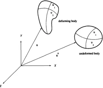
x(u, t) = [xl(u, t), x2(u, t), x3(u, t)]. The body in its natural

resting state is given by x°(u)= [x°(u), x°(u), x°(u)] (see where n = [ n l , n2, n3] is the unit surface normal. Two

Fioure 1).

The equations of motion for a deformable space curves have the same shape if their arc length s(x(u)), model can be written in Lagrangian form (which should curvature x(x(u)), and torsion ¢(x(u)) are identical forms of u = lull. See Reference 8 for a detailed discussion of hold for all u in the material domain Q) as

these formulations.

d ( ~x~ 0 x . 6e(x) ,., Using the above differential quantities, potential dt \ / z ~ - , / + y ~ - + - - ~ x =qx, t) (1) energies of deformation for use in Lagrange equations can be defined as the norm of the difference between the fundamental forms of the deformed body and those of where/~(u) is the mass density of the body at u, ~(u) is the undeformed body. This norm measures the amount the damping density of the body at u, f(x, t) is the net of deformation away from the natural shape so that the externally applied force, and ~(x) is the energy functional potential energy is zero when the body is in its natural which measures the net instantaneous potential energy shape and it increases as the model is increasingly of the elastic deformation of the body. deformed away from its natural shape.

The shape of a body is determined by the Euclidean If the fundamental forms associated with the natural distances between nearby points. As the body deforms, shape are denoted by the superscript 0, then the strain these distances change. Let u and u + du denote the energy for a curve can be defined as

material coordinates of two nearby points in the body.

~(X) = J n W I(S -- 80) 2 "1- W2(K -- K0) 2 + W3(~ " -- .~0)2 du

(5)

where w 1, w 2 and w 3 are the coefficients for the curve that show the amounts of resistance to stretching, bending, and twisting, respectively. The strain energy for a surface can be defined in a similar way:

8(x)-- f a IIG-G°II~, + IIB-B°II~, du x du 2 (6) where the weighted matrix norms I1" I1.~ and I1" I1.~ involve the weighting functions

w~(Ul, U2)

and

w~(ux, u2).

Analogously, a strain energy for a deformable solid is

~(x)= f a ]IG-G°]]~,

duxduldu3

(7) where the weighted matrix norm I1" I1,, involves the

z weighting functions wl~(Ul, u2, u3).

Figure 1 Geometric representation of deformable body for primal These energies denote the amount of energy required

Animation of deformable models: U G0d0kbay and B 0zg0q

The net external force in Lagrange's equations is the sum to rigid body dynamics to have a rigid body motion of various types of external force, such as gravitational besides its elastic motion) is given by

force and constraint forces.

The weighting functions in the above energies

q(u,t)=r(u,t)+e(u,t)

(8)

(w~j(Ux, U2)

and

w~(ut, u2)

for a deformable surface)

determine the properties of the simulated deformable Deformations are measured with respect to the reference material. The weighting function

w~(ul, u2) determines

shape r. Elastic deformations are represented by an surface tensions and shear strengths which minimize the energy e(e) which depends on the position of the body deviation of the surface's actual metric coefficients Gij frame ~b.

from its natural coefficients G °. As w~j is increased, the material becomes more resistant to length deformation,

with w~l and wl,2 determining this resistance along ul I M P L E ~ A T I O N O F P R I M A L and u2, and w121 = w2~ ~ determining the resistance to shear F O R M U L A ~ O N

deformation. The functions

w~(ul, u2) control surface

rigidities which act to minimize the deviation of the To simulate the dynamics of a deformable surface, we surface's actual curvature coefficients B 0 from its natural must discrctize the following expression for the elastic coefficients Bg.,~. As w~ is increased, the material becomes force, which is an approximation of the derivative of the more resistant to bending deformation, with w~l and we2 expression for potential energy:

determining this resistance along u l and u2, and w~2 = w, 2 1

determining the resistance to twist deformation. To & d / ~gx'~ d 2 / a 2 x \

simulate a stretch rubber sheet, for example, we make w~ ~x) = ~ - ~ / a 0 - - / + - - ~flo a--~u~) (9) relatively small and set w~=0. To simulate relatively i,i=t

\

auJ autuj

stretch resistant cloth, we increase the value of w~j. To where the functions ao(u, x) and fie(u, x) determine the simulate paper, we make w. 1. relatively large and we

'J elastic properties of the material. The expressions for introduce a modest value for w? Springy metal can be

_'J"

_aq(u,

x) and

#q(u, x) are as follows:

simulated 6 by increasing the value of w~.

To create animation with deformable models, the ao(u, x)=w~(uXGo-G °) (I0) differential equations of motion should be discretized by

applying finite difference approximation methods and

solving the system of linked ordinary differential

~q(u'x)=w~(uXBq-B°)

(11)

equations of motion obtained in this way. The diseretization of the expression for elastic force is achieved by applying the finite difference approximation

Hybrid formulation

method.

Since the body coordinates of the models are in the unit square domain, Qffi0~ul, uz~ < 1, we ~ t ~ this In this formulation, a deformable body is represented as domain as a regular M x N ~ t ¢ ~ of nodes, Here, the sum of a reference component r(Lt) and a

theint~modvspacingsareh~=l/Mandh2ffil/Ninthe

deformation component

e(u, t) (see Figure 2).

The Ul and u2 directions, respectively. The nodes on the positions of mass elements in the body relative to a body discrete model are indexed by integers Ira, n], where frame ~ (whose orion coincides with the body's centre 1 ~< m ~< M and 1 ~< n ~< N. Therefore, if x (which is a of mass and which should be evolved over time according continuous vector function x(u,t) represents the 3D coordinates of the positions of points, we d ~ e t i z e it by arrays of continuous time vector-valued nodal Y Deforming body variables xrCm, n] = x(mhx, nh2, t).

Since the elastic force requires the approximations to the first and second derivatives of the nodal variables, we should first define them for the vector-valued position function x.

The forward difference operators are

r y ~

D~x[ra, n] =(x[m+ 1, n]-x[m, n])/hl

(12)

/

Reference

x

compo~nt

D~x[ra,

n] =(x[m, n + 1] - x [ m ,

n])/h2

(13)

~dy ~ and the backward difference operators are

D-f x[m, n] =(x[m, n ] - x [ m - 1 ,

n])/h 1

(14)

X

1

~

/

D~x[m, n] = (x[m, n]--x[m, n-- 1])/h2

(15)

Using Equations 13 and 1 5, we can define the forward and backward cross difference operators as

z

D~2x[m, n] = D~-lx[m, n] =O~O~x[m, n]

Fillm~ 2 Geometric representation of deformable.body for hybrid =(xl'm+ 1, n + 1 ] - - x [ m + 1, n-I

Animation of deformable models: U GndOkbay and B Ozgfi 9

D~=x[m, n] = D~lx[m, n] = DiD~x[rn, n]

= (xEm, n]-xCm, n - 1 ) - x [ m - 1, n] +xEm-- 1, n - 1])/hlh e (17) and the central difference operators as

DllxCm, n] --D ~ D~ xCrn, n] -- xCm + 1, n] - 2x[m, n] + x [ m - 1, n])/h~

(18)

D22xC m, n] --D~D~xCm, n] = (x['m, n + 1] -- 2x[m, n] + xCm, n - 1-1)/h~ (19) Now, using the grid functions x[m, n], w~j[m, n], w~[m, n]

to represent their continuous counterparts, we can ~ . _

discretize the expressions in Equations 10 and 11 as Figure 3 Band structure of stiffness matrix K follows:

aij[m, n] = w~j[m, n](D + xCm, n] . D + xEm, n'l - G~[m, n])

(20) the total external force for that point. This method for calculating constraint forces gives good results for small

bu[m, n] =w~[m, n](nCm, n].D~xCm, n]-B~[m, n]) (21) time steps. For larger time steps, the model points are

subject to small oscillations since this approach corresponds to a corrective action.

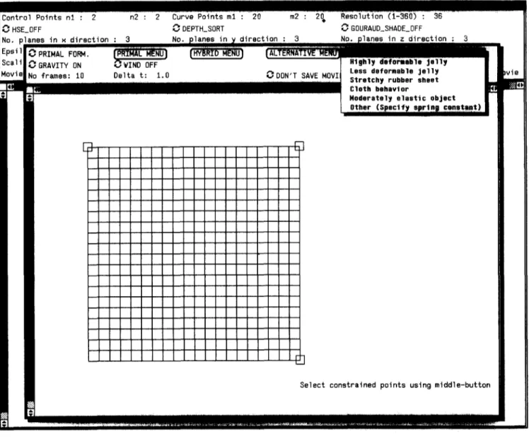
where the + superscript indicates that the forward cross The constrained points are specified by the user difference operator is used when i~j, and interactively. The system displays a grid specifying the body coordinates of each point existing in the model to n [ m , n ] = D~xCrn, n] x D~x[m,n] (22) be animated, and the user selects the points to be

ID~xCrn, n] x D~x[m, n-II constrained during the animation (the points that will

not move during the animation) using mouse buttons is the surface normal grid function. The elastic force in (see Figure 4). In other words, any point on a model can Equation 9 can be approximated as be constrained to a fixed location in space so that, when the model is animated, the constrained points remain in

2 their initial positions. The constraint force that connects

~[m, n] = ~ -Di(a~.~D+xCm, n])+D~(buD~x[m, hi) a material point u0 on a deformable model to a point Po

t.j= 1 in space by a spring is

(23)

f,(u, t) = k ( p o - X(Uo,

t))~(u-

Uo)

(25) To introduce free boundary conditions on the free edges

of a surface where the inner difference operators in where k is the spring constant and 6 is the unit delta Equation 23 attempt to access nodal variables outside function.

the discrete domain, we set the value of the inner The forces due to the collision of deformable models difference operators to zero. with impenetrable obstacles are calculated using the Expressing the grid functions x[m, n] and elm, nl as x obstacle's implicit (inside-outside) function. The obstacle and ~ in grid vector notation, where these denote the 31) exerts a repulsive force on the deformable model which posi/]ons of model points and elastic force for each model can be calculated as a function of the obstacle's implicit point stored in an M x N vector for an M x N discrete function such that the force increases quickly if the model grid of a deformable model, the elastic force can be written attempts to penetrate the obstacle. This is achieved by

in vector form as creating a potential energy function c exp(f(x)/O around

each obstacle, where f is the obstacle's implicit function,

= K(~).x (24) and c and ~ are constants determining the properties of

the obstacle. In our system, the user can select different where K is an M N x MN matrix. K is a sparse and banded obstacles to exist in an animation sequence by the help matrix. This becomes a major advantage when we solve of a menu. Ellipsoids, toroids and hyperboloids are the simultaneous system of 2nd-order ordinary differential possible choices for an obstacle. "l~he repulsive force due equations. The band structure of the matrix K is shown .to an impenetrable obstacle (expressed using the gradient

in Figure 3. V of the potential energy function) is

Then, we need to calculate the total external force for

each point of the model which is discretized using body f~(u, t)= -c((Vf(x)/0 e x p ( - f ( x ) / O , n)n (26) coordinates. In order to achieve this, we must add the

forces affecting a point: gravitational, viscous, collision where n(u, t) is the unit surface normal vector of the and constraint forces. The constraint forces are taken deformable body's surface.

into account in the following way. When a constrained The mass density p(Ul, u2) and the damping density point tends to move, an opposite force that will bring it ~(u~, u2) are discretized as grid functions p[m, n] and back to its original position is calculated and added to yl-m, hi. Let M be the mass matrix, and M N x MN

A n i m a t i o n of d e f o r m a b l e m o d e l s : U GiJdOkbay and B Ozg0q

J

k

I

!

:

I

Centre] Points nl : 2 ~ n2 : 2 Curve Points ml ~: 20 m2 2 ~ Res0iution 36 ...

HSE_OFF ~ DEPTH_SORT ~, GOURAUD_SHADE_0FF

,. pl ,si 1 : a l i

iiik:ii2kTiS!::=::

r l

Select constrained points using middle-button

Figure 4 Screen dump during specification of parameters for an animation

diagonal matrix with the #[m, n-I variables as diagonal procedure elements, and C be the damping matrix, constructed

similarly from ~,[m, hi. Then the Lagrang¢ equations can A,x, + a, =g, (30)

be expressed in grid vector form by the simultaneous

system of 2nd-order ordinary differential equations where the M N x M N matrix

d2x ~ + K(x)x = f(x) (27) - - \At ~ 2At

M ~ - ~ + C . . . .

At(xt)=K(xt)+(1.M+

1-~-C)

(31)

where the net external force on the surface f(ul, u2) has and the effective force vector been discretized into the grid vector f, which represents

the grid function f[m, n]. (~t2 )

We integrate -this system through time using a g , = f , + M + ~ I C ~ x , + ( 1 M - 1 C ~_, (32) 2At J - \ A t 2

step-by-step procedure. Evaluating K(x_) at time t + A t

and f at t, and substituting the discrete time with approximations

d2x X_t = (_x, - x,_ at)/At (33)

dt- f .~, (x, + at - 2 x t + x t - at)~ A t 2 (28)

Applying the above semiimplieit procedure, we can

dx evolve the dynamic solution from ~ven initial conditions

~tt.~(xt+at-x,_~,)/2At (29) Xo and _Xo at t=0. During each time step, we solve a

- - sparse linear algebraic system (Equation 30) for the

instantaneous configuration xt+at using the preceding into Equation 27, we obtain the semiimplicit integration solution xt and "_xt.

Animation of deformable models: U Gfid6kbay and B Ozg/ig:

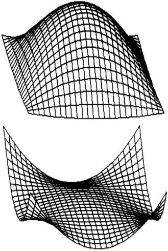
Figure 5 Highly nonrigid surface constrained from its four corners falls

The implementation of the hybrid formulation follows made up ofajeUy-like material. In this example, a discrete the same steps as those described for the primal model of size 20 x 20 is constrained from its four corners formulation. The only difference is that the sparse, banded and falls by the effect of gravitational force.

stiffness matrix K is constant. The equations of motion In

Figure 6,

we have used the hybrid formulation and can be expressed in semidiscrete form by a system of set the material properties to simulate a moderately rigid coupled ordinary differential equations. The system object (such as a thin metal plate). The model is contains two ordinary differential equations for the constrained from different points on its edges and a translational and rotational motion of the model as if all downward force is exerted on it. We can use such models of its mass were concentrated at its centre of mass, and in CAD and CAM applications to design mechanical parts. a system of ordinary differential equations whose size is In

Figure

7, a flat surface that is not resistant to proportional to the size of the discrete model. These elongation or contraction and not resistant to bending equations are solved in tandem for each time step with falls on an impenetrable obstacle which is a toroid. The respect to the initial conditions given, surface takes the shape of the toroid when it collides with

S I M U L A T I O N E X A M P L E S

We have implemented both primal and hybrid formulation in our system so that the user can interactively select between them. In this way, the primal formulation can be selected for highly nonrigid models, and the hybrid formulation can be selected for highly rigid models.

The system can be used to simulate the behaviour of elastically deformable materials, such as cloth, paper, and

metals. We can also utilize the system in CAD and

CAM

~

applications. For example, automobile bodies could be

designed by applying external forces to metal surfaces,

and imposing constraints on model points. " ~ ~

In

Figure 5,

we have used the primal formulation, and the material properties are adjusted to simulate a

membrane that is not resistant to elongation o r Figure 6 Thin metal plate constrained from three comers exerting a contraction, and not resistant to bending. The model is downward force

Animation of deformable models: U G~dOkbay and B OzgOq

Figure 7 Highly nonrigid surface collides with toroid

it. To obtain better results in collision simulations, we ' - - ~ - ' ~ ~--~

/ I

must either take a very small time step, or use adaptive ... !

time stepping. Otherwise, we may detect collisions very 3oooo / i

late, after the model points penetrate the obstacle too H Primal Formulation ... i

deeply. • ... • Hybrid Formulation /

r:"

25000 /

Q U A N T I T A T I V E C O M P A R I S O N O F F O R M U L A T I O N S

2OOOO

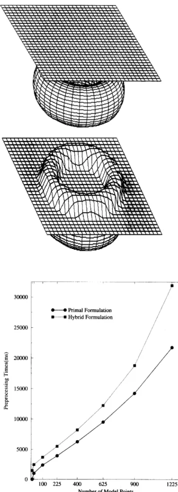
We have compared the processing times for generating /..U

an animation frame using the two formulations. T o ~z ....

compute processing times, simple B~zier surfaces are .- ~ / ...

animated using the two formulations. Fioures 8 and 9 ~ 15ooo ....

give the preprocessing and processing times of the =~ .,. ...

animations of the B~zier surfaces of different sizes. The ~ .... =

processing times for each frame given in the tables include 1oooo ... ././/

• the time taken to calculate the external forces for ... =

each model point . . . .

• the time taken to calculate the entries of the stiffness 5ooo . =

matrix*,

• the time taken to calculate the 3D positions of model "

points,

• the wireframe rendering time for the calculated frame. 0 ¢_{100 225} ~ ₄₀₀ ~ _{625 900 1225}

Number of Model Points

Although it seems from the graphs that the hybrid Figure 8 Preprocessing times using the two formulations formulation is superior to the primal formulation, they

complement each other for different elasticity properties. The nonquadric energy functional in primal formulation causes a nonlinear elastic force associated with the

*This is for the primal formulation; for the hybrid formulation, it is deformable body to appear in the partial differential

Animation of deformable models: U G5dDkbay and B OzgQ(~

3oooo . . . constructing the equations of motion for the models, the

equations should be solved using fast numerical methods. In this paper, we explained a system for animating H PrimalFormulation ff deformable models using a physically based approach. 25000 I---m Hybrid Formulation / The system uses both the primal formulation and the hybrid formulation for animating these models so that the user can decide which one to use in an animation, taking into consideration the advantages and

20000 _/ disadvantages of each formulation.

15000 R E F E R E N C E S

1 Giidiikbay, U and Ozgii~, B 'Free-form solid modeling using

d: ~ // deformations' Comput. & Graph. Vol 14 No 3 (1990) pp 491-500

100(~ - 2 Thalmann, N M and Thalmann, D 'Six-hundred indexed

references on computer animation' J. Visualization & Comput. Animat. Vol 3 No 3 (1992) pp 147-174

3 Platt, J and Barr, A H 'Constraint methods for flexible models' Comput. Graph. Vol 22 No 4 (1988) pp 279-288 (Proc. Siggraph '88)

5000 4 Pentland, A and Williams, J 'Good vibrations: modal dynamics

for graphics and animation' Comput. Graph. Vol 23 No 3 (1989) ... a pp 215-222 (Proc. Siggraph '89)

5 Witkin, A., Fleischer, K and Barr, A H 'Energy constraints on

. , , , , parameterized models' Comput. Graph. Vol 21 No 4 (1987)

0 100 225 400 625 900 1225 pp 225-232 (Proc. Siggraph '87)

Number of Model Points 6 Terzopoulos, D, Platt, J, Barr, A H and Fleischer, K 'Elastically deformable models' Comput. Graph. Vol 21 No 4 (1987) Figure 9 Processing times of one frame using the two formulations _{pp 205-214 (Proc. Sigoraph '87)}

7 Terzopoulos, D and Witkin, A 'Physically based models with rigid and deformable components' Comput. Graph. & Applic. Vol 8 No 6 (1988) pp 41-51

elastic force attempts to restore the shape of the deformed 8 Do Carmo, M P Differential Geometry of Curves and Surfaces body to a rest shape. The advantage of nonlinear Prentice-Hall, USA(1974)

elasticity is that it is in principle the most accurate way to characterize the behaviours of certain elastic phenomena. However, it can lead to serious practical

difficulties in the numerical implementation of deformable . . . U#ur Giidiikbay was born in Ni~de, models for animation. The hybrid formulation offers a Turkey, in 1965. He received a BSc in

practical advantage for fairly rigid models, whereas computer engineering from the Middle

primal formulation becomes unpractical because of the g u t Technical University, Turkey, in nonquadric energy functional with increasing rigidity 1987. He received an MSc and a PhD

and complexity of the models 7. from Bilkent University, Turkey, in

1989, and 1994, respectively, in the

An important advantage of primal formulation over Computer Engineering and lnformation

hybrid formulation is that it is easier to establish an Science Department. His research inter-

intuitive link between the weighting functions of the ests include physically based model-

deformable models and the resulting elastic behaviour, ling and animation, and deformable

. . . models.

This is because ofthe nature of the weighting functions.

C O N C L U S I O N S

Physically based modelling has emerged as a means of Biilent Ozgii¢ joined the Bilkent

creating realistic animation. It proposes methods of University Faculty of Engineering,

Turkey, in 1986. He is a professor of creating active models which react to applied forces, to computer science and the dean of the

constraints, to ambient media, or to impenetrable Faculty of Art, Design and Architecture.

obstacles, as one would expect from real physical objects. He has taught at the University of

In this way, computer animators are unconcerned with Pennsylvania, USA, the Philadelphia

College of Arts, USA, and the Middle

the kinematic details of animations, knowing that physics East Technical University, Turkey, and

will dictate the low-level motions, he worked as a member of the research

Physically based modelling adds new levels of staff at the Schlumberger Palo Alto

representation to object descriptions in addition to Research Center, USA. For the last 15 geometry. Forces, torques, velocities, kinetic and )'ears, he has been active in the field of computer graphics and animation. He received a BArch and an MArch in architecture, both potential energies, heat, and other physical quantities are from Middle East Technical University, Turkey, in 1972 and 1973. used to control the creation and evolution of models. To He received an M S in architectural technology from Columbia construct the differential equations of the motion of the University, USA, and a PhD in a joint program of architecture and models, different techniques, such as Lagrange equations computer graphics at the University of Pennsylvania, in 1974 and and constraint-based methods, could be used. After 1978.