IET Microwaves, Antennas & Propagation
Research Article
Analysis of a thin, penetrable, and
non-uniformly loaded cylindrical reflector
illuminated by a complex line source
ISSN 1751-8725 Received on 20th October 2016 Revised 3rd August 2017 Accepted on 14th August 2017 E-First on 4th October 2017 doi: 10.1049/iet-map.2016.0915 www.ietdl.org
Taner Oğuzer
1, Fadil Kuyucuoglu
2, Ibrahim Avgin
3, Ayhan Altıntaş
4 1Electrical and Electronics Engineering Department, Dokuz Eylul University, Buca, 35160 Izmir, Turkey 2Electrical and Electronics Engineering Department, Celal Bayar University, Muradiye, 45140 Manisa, Turkey 3Electrical and Electronics Engineering Department, Ege University, Bornova, 35100 İzmir, Turkey4Electrical and Electronics Engineering Department, Bilkent University, 06800 Ankara, Turkey
E-mail: [email protected]
Abstract: A thin, penetrable, and cylindrical reflector is illuminated by the incident field of a complex source point. The scattered
field inside the reflector is not considered and its effect is modelled through a thin layer generalised boundary condition (GBC). The authors formulate the structure as an electromagnetic boundary value problem and two resultant coupled singular integral equation system of equations are solved by using regularisation techniques. The GBC provides us to simulate the thin layer better than the resistive model which is applicable only for very thin sheets. Hence, the more reliable data can be obtained for high-contrast and low-loss dielectric material. The scattering and absorption characteristics of the front-fed and offset reflectors are obtained depending on system parameters. Also, the effects of the edge loading are examined for both E- and H-polarisations. The convergence and the accuracy of the formulation are verified in reasonable computational running time.
1 Introduction
The penetrable, thin, curved surfaces of lossy dielectric material have attracted considerable interest currently by researchers of electromagnetic scattering theory. One noticeable application is the reflectors used in the communication systems as microwave antennas. In the reflector antenna technology [1], they are generally made up of perfect electric conductor (PEC) type materials, but some resistive layers can also be applied to the edge of the reflector to reduce diffraction effects [2]. As another application, the frequency-selective surface (FSS) reflector antennas [3] are manufactured from the dielectric materials which allow waves to pass through in some frequencies. If the thickness is very small compared with the wavelength, the layer can be treated by a resistive BC. If the thickness is smaller than the 0.1λe where λe is
the wavelength, the single thin dielectric layer is called thin dielectric sheet (TDS) in the literature [4]. When the thickness of the thin dielectric layer is higher than the upper limit of the resistive case, it is needed to perform more accurate formulation to produce reliable numerical data.
In the simulation of TDS, an efficient approach is the dielectric physical optics (PO) [5, 6] as a high-frequency technique. The similar idea is generalised and applied to the three-dimensional (3D) reflectors having the multilayered structure as an extended PO [7]. PO can be improved by physical theory of diffraction (PTD) to model the edge waves by assuming the edges of the reflector as a local resistive half-plane. The asymptotic solution for scattering from a resistive half-plane is obtained in terms of Maliuzhinets functions. However, the high-frequency asymptotic solution for a thin layer half-plane thicker than the resistive case is not known. Therefore, the simple extension of PO to PTD is not easy. It should also be remarked that PO integral gives nearly correct result for a resistive case due to low diffraction effect.
One of the common techniques for the full-wave TDS simulation is to obtain a singular integral equation (SIE) on the reflector region and to solve it by the method of moments (MoM). For a TDS simulation, the volume integral equation (VIE) approach [8] is used to obtain MoM data with the tetrahedral-type basis functions. However, for the TDS, it produces some numerical errors because of the very flat tetrahedral production. To minimise this numerical error, one should increase the mesh density at the
expense of additional memory and run time. In another study in [9], the VIE-based MoM analysis is tried to prevent the previously mentioned numerical errors by using straight thin dipole-type basis functions carrying the sinusoidal current. Instead of the VIE, an old study given in [10] is improved by the proper numerical modelling of the field components varying along the normal direction of the TDS [4]. Recently, this study is generalised to solve multilayer TDS surfaces [11]. In [12], the wideband frequency domain solution of the TDS surface modelling is done with the combination of another method. Therefore, it seems that the wide spectrum of dielectric constants and the thicker layer in the thin surface modelling is still of interest among the electromagnetic community. On the other hand, lack of high accuracy and convergence are drawbacks of the SIE-based MoM solutions because of the level of the singularity and its handling techniques. Therefore, a special analytical handling of the singular parts of the original operator is still a serious alternative. This alternative is the method of the analytical regularisation (MAR) via the SIEs [13– 15].
The MAR technique is applied to the flat geometries to get accurate numerical data. The simulation of the resistive-dielectric strip of periodic flat gratings is cited in [16]. On the other hand, the thin layer generalised boundary condition (GBC) given in [17] can also be used for the sheets having more realistic thickness. For example, in [18], the SIE with its Nystrom-type solution is applied to a single material strip. In [19], different forms of the thin layer GBC are studied for a thin flat strip having low- and high-contrast dielectric permittivity and good accuracy is obtained by comparing the results with the Richmond's VIE data [20]. Recently in [21], the accuracy and limitations of the thin layer GBC are verified by using the Muller boundary integral equation method considering the material strip as an object. The thickness to width ratio of the strip is increased to quite larger values and it is seen that the thinner and wider strips show better agreement. In the recent paper [22], MAR technique is applied to the computational photonics problems.
A curved and thin impedance reflector having the non-circular profile is considered and the resultant two coupled systems of SIE are solved by a more accurate MAR technique [23]. The reflector is a smooth surface and locally planar. Then it is seen that the thin layer GBC [17, 19] can permit us to model the penetrable layers
having the larger thicknesses under the high-contrast approximation. The codes based on both PO and VIE-MoM are also produced. The VIE-MoM can be thought as an alternative of the full solution. It includes all physical effects. If the meshing level is taken as dense, we can assume it as a reference solution for comparison with other methods. The presented MAR code is possibly as accurate as the VIE-MoM and we can claim its accuracy, especially for the thin and moderate thicknesses under the thin layer GBC. Especially, Karlsson resistivity parameters can produce more accurate results [24]. It should also be mentioned that the presented MAR code has reasonable running times against the VIE-MoM. The PO is faster, but its accuracy is worse and it cannot be easily improved by PTD for the layer which is not very thin. Throughout the paper, e−iωt convention is used and
suppressed.
2 Description of basic equations
The 2D reflector surface M can be an arbitrary conic section with an offset orientation (Fig. 1). The d1, d2, and their corresponding angles φ1 and φ2 are the positions of lower and upper edges of the
reflector. The reflector thickness h is electrically very thin, i.e. h << λ, and it is made up of a dielectric material whose permittivity
εrφ can be non-uniformly distributed depending on φ. When the
reflector conic section is elliptic depending on the eccentricity (0 <
e < 1), the feed is located at the first focus point F1 and there is a second focus F2 at a far point. If the second focus goes to infinity, then only the first focus point remains and the reflector surface becomes a parabolic profile (e = 1). Then f is the focal length of the reflector. In making out our formulation, the open arc of the reflector contour M is extended to a complete closed contour C via arc S. This arc S is the combination of two separate portions, i.e.
S1−φ2, φ1 conic section part and S2 is the remaining
complementary circle of radius a. Also, L is the centre shift of this circle.
The requirements for a unique solution are the satisfaction of the Helmholtz equation, Sommerfeld radiation condition far from the reflector and the source; the GBC on M and the edge condition of the local energy finiteness in any finite domain enclosing the edge points. These conditions warrant the uniqueness of the solution [25].
The total tangential electric and magnetic fields on both sides of the thin layer can be stated as
E±(z,T)(r) = E(scz,±T)(r) + E(inz,T)(r) (1)
H(±T,z)(r) = H(scT,±z)(r) + H(inT,z)(r) (2)
where E(scz,T±) and H(scT,±z) represent scattered partial fields and E(inz,T),
H(inT,z) represent incident fields. Also the superscripts ‘±’ indicate
the front (+) and back (−) reflector faces. The subscript ‘T’ denotes the tangential field along t^. Here, the first term of the indices
appearing inside the subparentheses indicates the direction of the electric field in the E-polarisation case and the second term in the parentheses representing the direction of the magnetic field in the H-polarisation case. The E-field is taken along the z-direction and the H-field has a component along the tangential direction in E-polarisation.
The GBC for a thin surface can be written as [E(+z,T)(r) + E(−z,T)(r)]
2 = RT r n^(r) × [H−(T,z)(r) − H(+T,z)(r)] (3)
[H(+T,z)(r) + H(−T,z)(r)]
2 = ST r −n^(r) × [E−(z,T)(r) − E(+z,T)(r)] (4)
where RT(r) and ST r are defined as RT r = R r Z0 and
ST r = S r /Z0. The thin layer is characterised by this non-uniform
electrical resistivity RT and the magnetic resistivity ST. The free
space intrinsic impedance is denoted as Z0. n^ and t^ are the unit
normal and tangential vectors. The above boundary conditions can be obtained from the infinite slab geometries and then they can approximately be used for any smoothly curved surfaces when the radius of curvature is large [17]. In the case of a thin single-layer high-contrast material sheet, the resistivities (Mitzner type) can be given as RT φ = iZ20 ε1 rφ cot 1 2 εrφ k0h ST φ = i2Z 0 εrφ cot 12 εrφ k0h (5a)
It is assumed that εrφ >> 1 and k0h << 1 where k0 is the free
space wavenumber. Our reflector surface is thin single layer and the non-uniform permittivity variation in angle may exist [17].
An alternative to the approximate thin layer boundary condition is the compensated version of (5a) in terms of the thickness [24]. In this alternative, the thin layer has been replaced by a boundary condition that excludes the layer from the computation, but it keeps the thickness of the structure. Then the compensated version of the boundary condition is represented by the Karlsson resistivities
R∗φ = v − R − v2R
4vR − v2− 1
S∗φ = v − S − v2S
4vS − v2− 1
(5b)
where v = i cot(k0h/4) and R and S are normalised versions of the parameters given in (5a). Also RT∗ = R∗Z0 and ST∗= S∗/Z0.
Especially for thicker layers, Karlsson resistivities give more accurate results due to the proper phase correction and it is numerically studied in detail [21]. It is shown that these are valid for both low- and high-contrast cases again under the thin layer approximation. Even in the normal incidence, the Karlsson model gives the results very close to the exact one in magnitude and phase [24].
The incident electric field and the magnetic field will be written for both polarisations by the complex source point (CSP) method as follows:
Ukin(r) = H0(1)(k0r− rs), Vkin(r) =δikktk
0
∂Ukin(r)
∂n (6)
where the subscript k = e describes the E-polarisation case and k = h describes the H-polarisation case, also Uk = {Ez for k = e; Hz for k
= h} and Vk = {HT for k = e; ET for k = h}, δk = {1 for k = e; −1 for
k = h} and tk = {1/Z0 for k = e; Z0 for k = h}. The complex source
position vector rs is obtained from the real source position vector
r0(x0, y0) according to the CSP method. The complex source
position vector is defined as rs= r0+ ib that can be written as
rs= (x0+ ibcos β, y0+ ibsin β) expression where b and β are the
aperture width and beam-aiming angle, respectively. Note that the magnitude of the position vector of the CSP feed is complex-valued, as such rs= L2− b2+ i2Lbcos β but, only Re(rs) > 0
branch should be chosen for a physically meaningful case.
3 Formulation of the SIEs
We first write the scattered tangential electric and magnetic fields just on the front and back side of the reflector surface for both polarisations. Then by applying the initially defined GBC with the total fields for both sides, one can obtain the following SIEs on the material surface. These SIEs are given in (7) and (8) for E-polarisation case, (9) and (10) for H-E-polarisation case. Jz, MT and
JT, Mz are the electric and magnetic surface current densities
indicating the tangential field discontinuity on the thin layer surface for E- and H-polarisation cases, respectively. Furthermore,
G x = i/4 H01 x is the 2D Green's function. Each integral
equation constitutes a dual system with the zero surface current condition on the complimentary part S. So there are two coupled dual SIE systems in each polarisation. Also, the H-polarisation result can be obtained from E-polarisation by replacing the dual parameters. To do this, the electrical and magnetic resistivity values are interchanged
ik0Z0
∫
MJz(r′)G(k0|r − r′|) dl′ −∫
MMT(r′) ∂ ∂n′G(k0|r − r′|) dl′ + Ezin(r) = RT r Jz(r), r ∈ M (7) (see (8)) ik0 Z0∫
MMz(r′)G(k0|r − r′|) dl′ +∫
MJT(r′) ∂ ∂n′G(k0|r − r′|) dl′ + Hzin(r) = ST r Mz(r), r ∈ M (9)(see (10)) Suppose that the arbitrary conic section profile can be characterised by parametric equations in terms of the polar angle x = x(φ), y = y(φ) on MUS1 where −φ2< φ < φ2. We denote the
differential lengths in the tangential direction as ∂l = aβ(φ)∂φ. Here, β(φ) = r(φ)/(acos γ(φ)), r(φ) is the length of the position vector defined on the conic section part from the origin, ξ(φ) is the
angle between the normal and the x-direction, and γ(φ) is the angle
between the normal and radial direction. We set the surface-current densities to zero on S (slot). Thus, we can modify the above SIEs on the complete contour C made of M and S(S1US2) as such the
corresponding angle φ spans the whole period, that is, φ ∈ 0, 2π .
The radial parameter is given in piecewise manner in Table 1 for the whole contour C.
To proceed with the MAR-based formulation, all functions should be expressed in terms of the Fourier series (FS) form. The surface current densities are expanded into FS coefficients as follows: Jz Mz =n = − ∞
∑
∞ xne xnh e inφ, MT JT =n = − ∞∑
∞ mne mnh e inφ (11)Furthermore, to work with this way and make computations more economic, we add and subtract the similar functions from the original kernels. Then the corresponding FS coefficients can be computed by 2D-FFT algorithm efficiently and this provides us to solve reasonably larger geometries.
We used here a regularised solution different than the MoM and two dual SIE systems are obtained. In the discretisation procedure, the first dual system has the singular kernels having the lower singularity and it is in the Fredholm second kind stable form. For the second dual SIE system, the Riemann–Hilbert method is used for the regularisation. The more singular part of the original operator of the second dual SIE system is analytically inverted by the RHP technique that is also called semi-inversion procedure. Finally, an algebraic equation system is obtained with the remaining parts.
Then combining them leads to the following matrix equation:
∫
MJz(r′) ∂∂nG(k0|r − r′|) dl′ + ik 0 Z0∫
MMT(r′)cos ξ r − ξ r′ G(k0|r − r′|) dl′ + 1ik 0Z0∫
MMT(r′) ∂ 2 ∂l∂l′G(k0|r − r′|) dl′ +HTin(r) = ST r MT(r), r ∈ M (8) −∫
MMz(r′) ∂∂nG(k0|r − r′|) dl′ + ik0Z0∫
MJT(r′)cos ξ r − ξ r′ G(k0|r − r′|) dl′ + Z0 ik0∫
MJT(r′) ∂ 2 ∂l∂l′G(k0|r − r′|) dl′ + ETin(r) = RT r JT(r), r ∈ M (10)Table 1 Parameterisation of the problem geometry given in Fig. 1
Parameterisation of the closed contour C
−φ2< φ < φ2 (arbitrary conic section part) φ2< φ < 2π − φ2 (complementary circular part)
r(φ) = (1 + e) f1 + ecos(φ) γ = φ − sin−1 L
a sin φ , r(φ) = a2+ L2− 2aLcos γ
(If y(φ2) = d2 and x(φ2) = xe) L = −e
2x
e+ f (1 + e)e
1 − e2 a = f2(1 + e)2+ e2d22
I 0 0 I2Q× 2Q− . . . Q×Q . . . Q×Q . . . Q×Q . . . Q×Q Amnk 2Q× 2Q xnk mnk ynk = . .. . Bmk 1 × 2Q (12)
where the I is the identity matrix, Q= 2Ntr+ 1 and it is obtained
that ∑m∞,n= −∞|Amnk |2< ∞ and ∑m∞= −∞|Bmk|2< ∞, provided that
the branch cut associated with the CSP aperture does not cross the reflector contour M. In this case, the matrix equation system given in (12) is of Fredholm second kind. Hence, Fredholm theorems about the convergence and accuracy can be used.
4 Scattering and absorption characteristics
The scattering characteristics of a material reflector illuminated by a CSP feed are obtained by far-field radiation pattern. The total radiated field can be written asUktot= ϕinφ − k4 ϕ0a kscφ iπk20r eik0r (13) where ϕinφ = e−ik0r0cos φ−φ0ek0bcos φ−β (14) ϕsck φ = 1tk
∫
θ1 θ2 τkφ′ e−ik0r′ φ′ cos φ−φ′β φ′ dφ′ −δk∫
θ 1 θ2 ρkφ′ cos φ′ − γ′ − φ e−ik0r′ φ′ cos φ−φ′β φ′ dφ′ (15) where τk = {Jz for k = e; Mz for k = h}, ρk = {JT for k = h; MT for k =e}, and r0= x02+ y02 1/2, i.e. y0 = 0 and x0 = 0 in our case. The
incident field has been already defined previously by (6). The scattered field for both polarisations can be written by using the following integral: Ukscx, y = ikt0a k
∫
θ1 θ2 τkφ′ G x, y, φ′ β φ′ dφ′ −δka∫
θ1 θ2 ρkφ′ ∂G∂n′ β φ′ dφ′ (16) and Vkscx, y = −ikδktk 0 ∂Uksc ∂r (17)The required field components can be obtained by using (16) and (17) for the specified polarisation type. Besides x and y are the coordinates of the observation point in the near zone of the reflector surface. The total power radiated by the CSP feed in the presence of reflector is Pradk = Zπk00
∫
0 2π ϕinφ − k4 ϕ0a sck φ 2 dφ (18)The total radiated power is a function of the reflector material parameters as well as the source and reflector geometry parameters. Together with the absorbed power captured by the lossy penetrable surface, power conservation law must be satisfied in (19), whereas the power supplied by the CSP for both polarisation depending on k indices.
Psplk = P
radk + Pabsk (19)
The evaluation details of this supplied power are given in [15]. In computations, the power values are normalised by the power radiated by the same CSP source into free space, i.e. P0.
5 Numerical results
We present the radiation characteristics as such the radiation patterns, directivities, and power plots which are obtained by changing the various parameters of the presented formulation. For comparison, we also used PO technique for a thin dielectric layer [5–7]. We carried out our calculations using MATLAB® software
program in a PC with Intel i5 processor working on Windows 8 platform. We did not make any comparison with the commercial codes. Instead of this, we tried to make an explanation using the results produced from our own codes. Also, it should be said that the Mitzner and Karlsson boundary conditions are used in the numerical codes based on the FDTD technique as mentioned in [24]. The radiation patterns are obtained by using VIE-MoM and MAR (Karlsson), and the results are compared with each other. Generally, it is found that all patterns have similar characteristics.
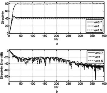
Fig. 2 shows the variation of the directivity with the increasing truncation number (Ntr) for E-polarisation. The relative error in
directivity is defined as ΔD = DNtr + 1− DNtr/ DNtr. The maximum
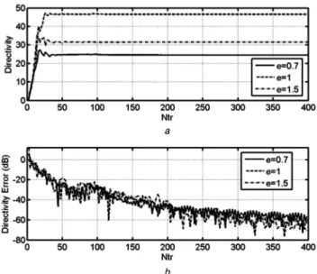
directivity is obtained for parabolic cross-section as expected. Similarly, Fig. 3 presents directivity and its relative accuracy for H-polarisation case with the smaller directivity levels than E-polarisation case. This drop is attributed to higher edge effects seen in H-polarisation. These two figures show that the convergence in directivity and the observable decrease in relative error can be guaranteed with increasing Ntr. This is a verification of the
statements that are the convergence and accuracy in the used regularised formulation of the presented problem. The wavelength in material is defined as λe= λ0/Re εr.
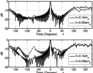
In Fig. 4, the layer thickness h is chosen as 0.25λe. By
considering the equivalent slab model at a point of the reflection on the surface, the maximum reflection coefficient is near unity. Then it is expected that the field should drop to smaller values at the back side of the reflector due to shadowing. In Fig. 4, the far-field radiation patterns are compared for the thin dielectric layer by using the present MAR (Karlsson) and the PO methods. The expected sharp drop at the back side is not observed. Also an increase is observed at the region between 40° and 70° in Fig. 4b.
Fig. 2 Directivity and relative directivity error comparisons for different eccentricity values(a) Directivity, (b) Relative directivity error versus truncation number (Ntr) for E-polarisation case. Problem parameters are
given as f = 10λ, d1 = −7.5λ, d2 = 7.5λ, kb = 5, h = 0.2λe, ɛr = 20 + 2i (L = 11.4λ, a = 21.35λ)
This situation is seen to be higher for thicker layers and observed for only for H-polarisation case. The interfering fields inside the layer become more dominant for thicker layers and even the stronger standing wave currents can occur. The side lobe increase between 40° and 70° in the radiation patterns can be attributed to these oscillatory currents.
The antenna patterns based on VIE-MoM and MAR are compared in Figs. 5–7 in terms of the increasing thickness and the relative permittivity. The relative permittivity values are taken as 4, 20, and 50 in the figures. Also the E-polarisation and the circular reflector cases are studied in these figures and the feed is located at the half distance of the radius. In Fig. 5, the thin reflector case is considered and h is taken as 0.15λe. If the εr is equal to 4 in Fig. 5a,
Mitzner resistivity result deviates from the others due to the relatively low level of the dielectric constant. In Figs. 5b and c, all results almost close to each other under the high-contrast approximation. It is seen that the field passes through the reflector along the backward direction due to the high transmission property of this transparent sheet.
In Fig. 6, the thickness h is 0.25λe. The expected shadowing in the magnitude of the field is not observed in both methods of
VIE-MoM and the MAR (Karlsson type). This is similar to the parabolic reflector results given in Fig. 4. When we did not consider the Mitzner results, VIE-MoM and the presented MAR are very similar. The VIE-MoM solution is performed by using the pulse type basis functions which are chosen inside the thin dielectric reflector. The circular geometry has a shift-invariant structure along angular direction. We followed the Galerkin's procedure with this Toeplitz symmetry of the circular case along angular direction and we computed the appearing integrals sensitively. Normally the MoM directivity has not so converged in terms of problem dimension (see Table 2, small variation), but the MoM code is faster for 2 radial divisions. However to obtain more accurate results, we should take high discretization level (N = 800 along angular and Nr = 5 along radial), then it becomes slower compared to the MAR. We consider this dense MoM results for comparing purposes. Since the MoM formulation is full and all physical effects should be included. Furthermore, the recordable shadowing at the back side is not observed here and the field level is not too small like seen in the perfectly conducting reflectors. It may not be seen because the infinite slab model is changed near the edges. The field can penetrate inside the material and radiate
Fig. 3 Directivity and relative directivity error comparisons for different eccentricity values(a) Directivity, (b) Relative directivity error versus truncation number (Ntr) for H-polarisation case. Problem parameters are
given as f = 10λ, d1 = −7.5λ, d2 = 7.5λ, kb = 5, h = 0.2λe, ɛr = 20 + 2i (L = 11.4λ, a = 21.35λ)
Fig. 4 Normalised far-field radiation patterns versus angle in degrees for MAR (Karlsson) and PO solutions(a) E-polarisation and (b) H-polarisation cases. Problem parameters are given as f = 10λ, d1 = −7.5λ, d2 = 7.5λ, e = 1, kb = 2, h = 0.25λe, ɛr = 20 + 3i (L = 11.4λ, a = 21.35λ)
Fig. 5 Comparison of the normalised far-field radiation patterns for E-polarisation using MoM and MAR (a) εr = 4, (b) εr = 20, (c) εr = 50 case. The solid line is VIE-MoM, the dashed line is Mitzner resistivity case, and the dotted line is Karlsson resistivity case. Problem parameters are given as f = 20λ (radius of the reflector), r0 = f/2 (feed position), e = 0 (circle), h = 0.15λe, d1 = −7.5λ, d2 = 7.5λ, kb = 2 (L = 0, a = 20λ)
Fig. 6 Comparison of the normalised far-field radiation patterns for E-polarisation using MoM and MAR (a) εr = 4, (b) εr = 20, (c) εr = 50 case. The solid line is VIE-MoM, the dashed line is Mitzner resistivity case, and the dotted line is Karlsson resistivity case. Problem parameters are given as f = 20λ (radius of the reflector), r0 = f/2 (feed position), e = 0 (circle), h = 0.25λe, d1 = −7.5λ, d2 = 7.5λ, kb = 2 (L = 0, a = 20λ)
through the back region. Therefore, complicated interactions on the curved thin sheet may occur. Also increasing the relative dielectric constant of the layer reduces the back field around 2–3 dB. Since the field reduction is expected inside the layer. This observation also supports our claim.
In Fig. 7, the thickness h is 0.4λe. The thin layer approximation
becomes to deviate and naturally all results become different and this is seen dominantly in Fig. 7a. When we increase the dielectric constant, it again makes the electrical thickness lower and the deviation between the methods reduces as seen in Figs. 7b and c.
Next we increased the discretisation level close to our computer memory capacity and the results are presented in Table 2. As it is seen, the overall running times are greater for the VIE-MoM. However, there is not much difference in the CPU times because we write our MoM code for the circular and shift-invariant case. If one performs the similar analysis for the parabolic surface, the big difference will appear in the running times. The directivity is almost in the same level in the VIE-MoM and the presented MAR results. However, it is seen in Table 2, MoM has a slow convergence, so it needs the dense mesh for the proper comparison. Therefore, we observe that the presented MAR gives quick and accurate results.
The far-field radiation patterns with two different polarisations are presented in Figs. 8a and b for the offset parabolic reflector. The results are obtained from the MAR code using the Karlsson coefficients. One can say that the computed radiation level drops 2–3 dB for the backside angles of the reflector. However, this field level drop is not observed in H-polarisation. This can be explained that even the reflection is high; the stronger surface interactions for H-polarisation produce the extra field level in the backside region. Also, an increase is observed at the region between −150° and −30° in Fig. 8b. This situation was also seen in Fig. 4 as discussed in the related sentences.
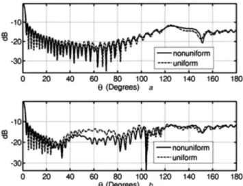
The results for Figs. 9 and 10 are obtained from the MAR code using Mitzner parameters which are very close to Karlsson for this thin case. Having presented uniform dielectric case, we disclose non-uniform edge loading effect by changing dielectric material properties. This edge loading is computed by decreasing the relative permittivity linearly from middle region value εrm = 70 + 5i
to the edge point value εre= 10 close to the edge [15]. It is expected
that this variation decreases edge effects. Far-field patterns of E-and H-polarisations with uniform E-and non-uniform edge loadings are given in Figs. 9a and b. Field levels are reduced in the non-uniform case for both figures especially in 30° and 110° region. However, in H-polarisation, the radiation level drop is larger as expected. By this non-uniformity, the edge effects are reduced, but this is high for Fig. 9b because the edge effects are stronger for H-polarisation.
We further study the scattered and absorbed power variations by changing the problem parameters. Fig. 10 describes the total radiated and absorbed normalised powers and even the forward
Fig. 7 Comparison of the normalised far-field radiation patterns for E-polarisation using MoM and MAR
(a) εr = 4, (b) εr = 20, (c) εr = 50 case. The solid line is VIE-MoM, the dashed line is Mitzner resistivity case, and the dotted line is Karlsson resistivity case. Problem parameters are given as f = 20λ (radius of the reflector), r0 = f/2 (feed position), e = 0 (circle), h = 0.4λe, d1 = −7.5λ, d2 = 7.5λ, kb = 2 (L = 0, a = 20λ)
Table 2 CPU time comparison of MAR (Karlsson), MOM, and PO with the problem parameters are given as f = 20λ (radius of
the reflector), r0 = f/2 (feed position), e = 0 (circle), d1 = −7.5λ, d2 = 7.5λ, kb = 2, ɛr = 20, (L = 0, a = 20λ), h = 0.25λe. The memory
complexity of MAR is O(2(2Ntr+ 1)) and for MoM O(NrN) where N is the angular and Nr is the radial division of the thin circular
region. In PO, N is indicating the total division during the computation of PO integral by using Riemann sum
MAR MOM (Nr = 2) MOM (Nr = 3) PO
CPU time Directivity CPU time Directivity CPU time Directivity CPU time Directivity
N = Ntr = 100 23.75 61.85494 63.70 61.86084 131.93 61.69595 12.44 38.69443 N = Ntr = 150 36.46 62.16126 94.35 61.39400 196.32 61.22968 18.15 40.21739 N = Ntr = 180 44.36 61.39103 111.98 61.68380 229.25 61.51296 21.56 40.32571 N = Ntr = 215 60.17 62.25092 132.57 59.40750 269.32 59.18424 25.66 40.54473 N = Ntr = 250 77.86 62.88699 154.42 61.41820 313.31 61.24567 31.13 40.70104 N = Ntr = 280 99.00 62.99154 174.02 60.82979 351.83 60.64498 42.10 40.71696 N = Ntr = 320 136.88 61.70833 189.37 59.33942 378.66 59.30603 42.35 40.90919 N = Ntr = 380 207.00 61.65374 201.12 61.70965 404.28 61.52647 52.01 40.89937 N = Ntr = 430 283.68 62.33127 219.47 61.41234 436.66 61.23629 57.29 40.75923 N = Ntr = 470 359.99 62.64481 234.58 61.22631 469.07 61.04846 66.55 40.88781
Fig. 8 Normalized far-field radiation patterns versus angle in degree for reflector geometry as an offset type
(a) E-polarisation, (b) H-polarisation cases. Problem parameters are given as f = 15λ, d1 = 5λ, d2 = 20λ, β = φ1+ φ2/2, e = 1, kb = 3, εr = 20 (L = 21.66λ, a = 36λ)
directivity versus the complex part of the relative permittivity εr.
The variable parameter η is defined as εr= 20 1 + iη . The electric
field strength inside the thin layer is stronger in E-polarisation, so the absorbed power is greater in this case. Consequently, the radiated power level in E-polarisation is small. Figs. 10a and b confirm our claims. In Fig. 10b, there is a critical η value that makes absorbed power maximum. If we increase η, the absorbed power starts to incline and reaches 0 when η → ∞ (PEC). The forward directivity increases with the increasing η because the reflector surface approaches to PEC case as shown in Fig. 10c. However, the directivity becomes smaller for H-polarisation again due to the higher scattering of the waves from the reflector due to the dominant edge effects.
6 Summary and conclusion
A thin and penetrable cylindrical reflector illuminated by CSP is studied by using the thin layer GBC. The properties of the model are clearly verified in our numerical results. The total scattering and absorbed power plots are shown and also the radiation patterns are compared with the extended PO and VIE-MoM solutions. We
see that the field levels do not drop much in the backside region. This may be due to the complicated interactions of the waves in and on the surface of the thin reflector. There are many studies for very thin resistive layers in the literature, whereas studies of thicker layers are very few. Here, more realistic curved reflectors having high-contrast dielectric constant through the SIEs-based MAR solution are simulated. Our reliable computed data can be used in the design of transparent thin reflectors.
7 References
[1] Scott, C.R.: ‘Modern methods of reflector antenna analysis and design’ (Artech House, Norwood: MA, 1990)
[2] Jenn, D.C., Rusch, W.V.T.: ‘Low-side lobe reflector synthesis and design using resistive surfaces’, IEEE Trans. Antennas Propag., 1991, 39, (9), pp. 1372–1375
[3] Rahmat-Samii, Y., Tulintseff, A.N.: ‘Diffraction analysis of frequency selective reflector antennas’, IEEE Trans. Antennas Propag., 1993, 41, (4), pp. 476–487
[4] Chiang, I.T., Chew, W.C.: ‘Thin dielectric sheet simulation by surface integral equation using modified RWG and pulse bases’, IEEE Trans. Antennas Propag., 2006, 54, (7), pp. 1927–1934
[5] Janse van Rensburg, D.J., Malherbe, J.A.G., McNamara, D.A.: ‘Computation of electromagnetic plane-wave scattering from a curved dielectric shell using a physical optics approach’, Microw. Opt. Technol. Lett., 1992, 5, (7), pp. 326–328
[6] Hodges, R.E., Rahmat-Samii, Y.: ‘Evaluation of dielectric physical optics in electromagnetic scattering’. IEEE AP Society Int. Symp. Proc., Ann Arbor, USA, June 1993, pp. 1742–1745
[7] Ip, H.-P., Rahmat-Samii, Y.: ‘Analysis and characterization of multilayered reflector antennas: rain/snow accumulation and deployable membrane’, IEEE Trans. Antennas Propag., 1998, 46, (11), pp. 1593–1605
[8] Schaubert, D.H., Wilton, D.R., Glisson, A.W.: ‘A tetrahedral modeling method for electromagnetic scattering by arbitrarily shaped inhomogeneous dielectric bodies’, IEEE Trans. Antennas Propag., 1984, 32, (1), pp. 77–85 [9] Pelletti, C., Bianconi, G., Mittra, R., et al.: ‘Volume integral equation analysis
of thin dielectric sheet using sinusoidal macro-basis functions’, IEEE Antennas Wirel. Propag. Lett., 2013, 12, pp. 441–444
[10] Harrington, R.F., Mautz, J.R.: ‘An impedance sheet approximation for thin dielectric shells’, IEEE Trans. Antennas Propag., 1975, 23, (4), pp. 531–534 [11] Niu, X., Nie, Z., He, S., et al.: ‘Improved multilayer thin dielectric sheet
approximation for scattering from electrically large dielectric sheets’, IEEE Antennas Wirel. Propag. Lett., 2015, 14, pp. 779–782
[12] Jeong, Y.-R., Hong, I.-P., Lee, K.-W., et al.: ‘‘Fast frequency sweep using asymptotic waveform evaluation technique and thin dielectric sheet approximation’, IEEE Trans. Antennas Propag., 2016, 64, (5), pp. 1800–1806 [13] Nosich, A.I.: ‘The method of analytical regularization in wave-scattering and eigenvalue problems: foundations and review of solutions’, IEEE Trans. Antennas Propag. Mag., 1999, 41, (3), pp. 34–49
[14] Oğuzer, T., Altintas, A., Nosich, A.I.: ‘Integral equation analysis of an arbitrary profile and varying-resistivity cylindrical reflector illuminated by an E-polarized complex source-point beam’, J. Opt. Soc. Am. A, 2009, 26, (7), pp. 1525–1532
[15] Oğuzer, T., Altıntaş, A., Nosich, A.I.: ‘Analysis of the elliptic-profile cylindrical reflector with a varying resistivity using the complex source and dual-series approach: H-polarization case’, Opt. Quantum Electron., 2013, 45, (8), pp. 797–812
[16] Zinenko, T.L., Nosich, A.I., Okuno, Y.: ‘Plane wave scattering and absorption by resistive-strip and dielectric-strip periodic gratings’, IEEE Trans. Antennas Propag., 1998, 46, (10), pp. 1498–1505
[17] Bleszynski, E., Bleszynski, M.K., Jaroszewicz, T.: ‘Surface integral equations for electromagnetic scattering from impenetrable and penetrable sheets’, IEEE Trans. Antennas Propag., 1993, 35, (6), pp. 14–25
[18] Shapoval, O.V., Sauleau, R., Nosich, A.I.: ‘Scattering and absorption of waves by flat material strips analyzed using generalized boundary conditions and Nystrom-type algorithm’, IEEE Trans. Antennas Propag., 2011, 59, (9), pp. 3339–3346
[19] Shapoval, O.V., Sauleau, R., Nosich, A.I.: ‘Fabry-Perot-like resonances in the E-polarized electromagnetic plane wave scattering and absorption by a thin dielectric strip’. 6th European Conf. on Antennas and Propagation (EUCAP), Prague, Czech Rep., March 2012, pp. 655–658
[20] Richmond, J.H.: ‘Scattering by thin dielectric strips’, IEEE Trans. Antennas Propag., 1985, 33, (1), pp. 64–68
[21] Sukharevsky, I.O., Shapoval, O.V., Altintas, A., et al.: ‘Validity and limitations of the median-line integral equation technique in the scattering by material strips of sub-wavelength thickness’, IEEE Trans. Antennas Propag., 2014, 62, (7), pp. 3623–3631
[22] Nosich, A.I.: ‘Method of analytical regularization in computational photonics’, Radio Sci., 2016, 51, (8), pp. 1421–1430
[23] Kuyucuoglu, F., Oğuzer, T., Avgin, I., et al.: ‘Analysis of an arbitrary-profile, cylindrical, impedance reflector surface illuminated by an E-polarized complex line source beam’, J. Electromagn. Waves Appl., 2014, 28, (3), pp. 360–377
[24] Karlsson, A.: ‘Approximate boundary conditions for thin structures’, IEEE Trans. Antennas Propag., 2009, 57, (1), pp. 144–148
[25] Colton, D., Kress, R.: ‘Integral equation method in scattering theory’ (Wiley, New York, 1983)
Fig. 9 Normalised far-field radiation patterns versus angle in degrees for uniform and non-uniform cases with h = 0.15λe (a) E-polarisation,
(b)H-polarisation cases. Problem parameters are given as f = 15λ, d1 = −12.5λ, d2 = 12.5λ, e = 1, kb = 3, εrm= 70 + 5i, εre= 10, linear drop from εrm to εre
near edge (L = 17.6λ, a = 32.5λ)
Fig. 10 Radiation characteristics comparisons for E- and H- polarisations
(a) Normalised radiated power, (b) Normalised absorbed power, (c) Forward directivity versus η for E-polarisation (dashed curve) and H-polarisation (solid curve) cases. Problem parameters are given as f = 10λ, d1 = −7.5λ, d2 = 7.5λ, e = 1, kb = 3, h = 0.15λe (L = 11.4λ, a = 21.35λ)