Analytical regularization based analysis of a spherical reflector symmetrically illuminated by an acoustic beam

Analytical regularization based analysis of a spherical reflector

symmetrically illuminated by an acoustic beam

Sergey S. Vinogradova) and Elena D. Vinogradovab)

Department of Mathematics, University of Dundee, Dundee DD1 4HN, Scotland, United Kingdom

Alexander I. Nosich

Institute of Radiophysics and Electronics of the National Academy of Sciences, Ul. Proskury 12, Kharkov 310085, Ukraine

Ayhan Altintas¸

Department of Electrical and Electronics Engineering, Bilkent University, 06533 Ankara, Turkey 共Received 3 April 1999; revised 16 February 2000; accepted 18 February 2000兲

A mathematically accurate and numerically efficient method of analysis of a spherical reflector, fed by a scalar beam produced by a complex source-point feed, is presented. Two cases, soft and hard reflector surface, are considered. In each case the solution of the full-wave integral equation is reduced to dual series equations and then further to a regularized infinite-matrix equation. The latter procedure is based on the analytical inversion of the static part of the problem. Sample numerical results for 50-␭ reflectors demonstrate features that escape a high-frequency asymptotic analysis. © 2000 Acoustical Society of America.关S0001-4966共00兲00306-4兴

PACS numbers: 43.20.Fn关ANN兴

INTRODUCTION

Most frequently, performance of a reflector antenna is predicted by using asymptotic high-frequency techniques such as Physical Optics 共PO兲, combined with Geometrical Theory of Diffraction 共GTD兲,1,2for the off-beam radiation. The Method-of-Moments共MoM兲 is also used in the integral-equation共IE兲 analysis of reflectors of small to moderate size in terms of wavelength.3,4The merits and limitations of both approaches are well known. In spite of their flexibility, PO or GTD alone is not uniformly accurate with respect to the di-rection in space, and both fail to characterize smaller reflec-tors. MoM algorithms for the full-wave IE become compu-tationally expensive for larger reflectors, due to either large matrices or a large time for filling the matrix. Besides, not every MoM approximation scheme is convergent to the exact result as the number of equations is increased, in the sense that the computation error cannot be progressively mini-mized.

The feed field is normally simulated via a Gaussian beam or a spherical-wave expansion multiplied with an an-gular window function. Commonly it is neglected by these simulations that such a feed field function does not solve the Helmholtz equation exactly, although the radiated or scat-tered field is found as a solution of the full-wave integral equation. It has been proposed therefore to use the complex source-point共CSP兲 beam, or combination of such beams, as a feed field.5,6 Then, the latter is an exact solution to the Helmholtz equation at every point in the physical observa-tion space. In Refs. 7, 8, this concept was combined with PO and GTD for a characterization of a spherical-wave scalar

beam scattering from a circular aperture. This concept is fur-ther developed in Refs. 9, 10, which contain practical and useful results.

In a recent study,11it was demonstrated, for a 2D prob-lem, that a very accurate and computationally efficient analy-sis of reflector antennas can be achieved by using a combi-nation of the CSP method to simulate a beam-like feed field, and an analytical regularization based technique to solve the reflector scattering. In Ref. 11, a circular-cylindrical reflector fed by the CSP-type line sources was considered. First, the IE was discretized into the dual series equations 共DSE兲 in terms of the entire-period angular exponents. Then, the static part of DSE was analytically inverted, using the Riemann– Hilbert Problem solution, resulting in an infinite matrix Fred-holm equation of the second kind. A remarkable feature of this equation is that it can be solved numerically with a guar-anteed accuracy and small CPU time expenditures.

Our present study is similar to Ref. 11, but deals with a quasi-3D problem of a spherical reflector. Acoustic reflectors of this type have been analyzed in Refs. 12, 13 assuming finite transparency of reflector material and tapered spherical wave illumination. Unlike Refs. 12, 13, we characterize the feed by a scalar CSP beam, assume the reflector to be per-fectly hard or soft, and develop a numerically exact solution. It is obtained from the DSE in terms of Legendre polynomi-als, with the static part inversion based on the Abel integral equation technique.14,15This solution is equivalent to a judi-cious choice of the expansion functions in an MoM proce-dure, forming a set of the orthogonal eigenfunctions of the static limit of the IE kernel. The usage of a directive CSP field as a feed brings new features, hence we believe that an in-depth physical analysis of two scalar problems of soft and hard reflectors is reasonable. To obtain the results which are applicable to paraboloidal reflectors as well, we restrict the computed examples to ‘‘dish’’ reflectors with a large to

mod-a兲_{Visiting Scientist from Kharkov Academy of Civil Engineering,} Kharkov 310002, Ukraine.

b兲_{Visiting Scientist from Institute of Radiophysics and Electronics NAS,} Kharkov 310085, Ukraine.

erate f /d ratio 关 f and d being the Geometrical Optics 共GO兲 focal distance and the dish diameter, respectively兴.

The remainder of the paper is organized as follows. In Sec. I, we formulate the boundary-value problem for soft and hard reflectors, and derive a rigorous IE for each case. Fur-ther we discretize and convert it to the DSE. In Sec. II, we present basic points of the partial inversion of the DSE and reduction to the regularized matrix equation. Section III con-tains the formulas for far field characteristics. Section IV presents the results of numerical analysis concerning radia-tion patterns and the directivity of the soft and hard spherical reflectors. Conclusions of the presented work are summa-rized in Sec. V. Focal shifts in parabolic reflectors. A note should be made that the time dependence is assumed as e⫺i␻tand is omitted.

I. FORMULATION AND BASIC EQUATIONS A. Problem formulation

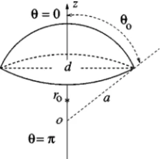
Consider a zero-thickness, perfectly soft or perfectly hard, spherical reflector of radius a and angular width 2␪0, symmetrically excited by the field of a CSP beam. That is, the feed is located at the point (r_s,0,0) with the radial source coordinate being a complex value: r_s⫽r₀⫹ib. The geom-etry of the problem is shown in Fig. 1. The incident scalar wave field is:

U0共r,␪兲⫽eikR/R, 共1兲

where R⫽(r2⫺2rrscos␪⫹rs

2

)1/2, and k⫽␻/c is the real-valued free-space wave number (c being the sound propaga-tion velocity兲. The scattered field Usc(r,␪) is the solution of a boundary-value problem for the 3D Helmholtz equation, with the boundary condition of either soft or hard type at the reflector surface M: (r⫽a,0⭐␪⬍␪0,0⭐␸⭐2␲)

U0⫹Usc兩M⫽0,

⳵共U0_⫹Usc_兲 ⳵r

冏

M

⫽0. 共2兲

The formulation must also include共i兲 the edge condition Usc⬃O(␳1/2), ⳵Usc/⳵r⬃O(␳⫺1/2), where ␳→0 is the dis-tance from the dish rim, and 共ii兲 the outgoing radiation con-dition at r→⬁, to ensure the solution uniqueness.16

B. Acoustically soft reflector

Consider first the case of a perfectly soft reflector. We seek the scattered field function as a single-layer potential:

Usc共r兲⫽⫺ 1 4␲

冕 冕

M

js共␪

⬘

,␸

⬘

兲

eik兩r⫺r⬘兩

兩r⫺r

⬘

兩 dS

⬘

, 共3兲 where 兩r⫺r

⬘

兩⫽兵r2⫹a2⫺2ra关cos␪

⬘

cos␪⫹sin␪

⬘

sin␪ ⫻cos(␸⫺␸

⬘

)兴其1/2 is the distance between the observation point and a point at the reflector surface. Note that the un-known density function is related to the jump of the scattered field normal derivative across the reflector as

js共␪

⬘

,␸

⬘

兲⫽ ⳵Usc ⳵r

冏

r⫽a⫹0 ⫺⳵U sc ⳵r

冏

r⫽a⫺0 . 共4兲

The soft-surface boundary condition Eq. 共2兲 then yields a Fredholm first kind IE as

a 8␲

冕

0 ␪0

冕

0 2␲ js共␪

⬘

,␸

⬘

兲 ei2ka兩sin(␺/2)兩 兩sin共␺/2兲兩 sin␪

⬘

d␪

⬘

d␸

⬘

⫽U0_{共a,␪,␸兲, 共5兲}

where␺⫽arccos关cos␪

⬘

cos␪⫹sin␪

⬘

sin␪cos(␸⫺␸

⬘

)兴. Instead of approximating IE Eq. 共5兲 by MoM with sub-domain or M-sub-domain basis functions, we further discretize it in terms of a complete set of orthogonal functions in the global domain 0⭐␪⭐␲. In our case of a ␸-independent solution, such a set is formed by the Legendre polynomials P_n(cos␪) (n⫽0,1,2, . . . ). By extending the density function to be identically by zero on the complementary surface (r ⫽a,␪0⬍␪⭐␲), as is natural due to Eq.共4兲, we assume that for all ␪

⬘

js共␪

⬘

兲⫽⫺ 1 ka2 n

兺

⫽0 ⬁ xn s_{共2n⫹1兲P} n共cos␪

⬘

兲, 共6兲

with the expansion coefficients x_ns, n⫽0,1,2, . . . to be found.

Besides, it is known that the free-space Green’s function can be expanded as:15

eik兩r⫺r⬘兩 兩r⫺r

⬘

兩⫽ikm

兺

_⫽0 ⬁ 共2⫺␦0m兲cos m共␸⫺␸

⬘

兲 ⫻

兺

n⫽m ⬁ 共2n⫹1兲共n⫺m兲!_共n⫹m兲! ⫻

再

hn (1) 共ka兲jn共kr兲, r⬍a j_n共ka兲h_n(1)共kr兲, r⬎a

冎

⫻Pn m 共cos␪兲Pn m 共cos␪

⬘

兲, 共7兲

where P_nmare the associated Legendre functions. This yields the following series representation of the kernel function of the IE Eq.共5兲: ei2ka兩sin(␺/2)兩 兩sin共␺/2兲兩 ⫽i2kam

兺

⫽0 ⬁ 共2⫺␦0m兲cos m共␸⫺␸

⬘

兲 ⫻

兺

n⫽m ⬁ 共2n⫹1兲共n⫺m兲!_共n⫹m兲!jn共ka兲hn (1)_共ka兲 ⫻Pn m_{共cos␪兲P} n m_共cos␪

_⬘

_{兲. 共8兲}

Now the integration in Eq.共5兲 over␪

⬘

can be extended from 0 to ␲. This enables us to use orthogonality of the spherical harmonics

冕

0 2␲ cos m共␸⫺␸

⬘

兲

冕

0 ␲

Ps共cos␪

⬘

兲Pn共cos␪

⬘

兲sin␪

⬘

d␪

⬘

d␸

⬘

⫽_{共2n⫹1兲)共s⫺m兲!}4␲共s⫹m兲! ␦ns␦m0 共9兲

when discretizing the IE. Together with the specification that the density function Eq. 共6兲 is zero off the reflector, this brings us to the dual series equations共DSE兲:

兺

n⫽0

⬁

x_ns共2n⫹1兲j_n共ka兲h_n(1)共ka兲P_n共cos␪兲

⫽

兺

n⫽0 ⬁ b_nsP_n共cos␪兲, 0⭐␪⬍␪₀, 共10兲

兺

n⫽0 ⬁ x_ns共2n⫹1兲Pn共cos␪兲⫽0, ␪0⬍␪⭐␲,

where the right-hand side coefficients are determined by the CSP feed field as

b_ns⫽共2n⫹1兲jn共krs兲hn

(1)_{共ka兲. 共11兲}

Once again, the DSE Eq. 共10兲 can be attacked by a ’’brute force’’ numerical solution with a direct MoM scheme. Al-though the results are generally meaningful, only a few cor-rect digits can be obtained, and there is no possibility of increasing accuracy by taking a greater number of colloca-tion points. That is our motivacolloca-tion for regularizing the DSE Eq. 共10兲, to obtain an algorithm convergent to the exact so-lution in a pointwise manner.

C. Acoustically hard reflector

For a perfectly hard spherical reflector fed by a CSP feed, we seek the scattered field function as a double-layer potential: Usc共r兲⫽⫺ 1 4␲

冕 冕

M jh共␪

⬘

,␸

⬘

兲 ⳵ ⳵r

⬘

再

eik兩r⫺r⬘兩 兩r⫺r

⬘

兩

冎

dS

⬘

, 共12兲 where the ␸-independent density function is now related to the jump of the field across the reflector surface:

jh共␪

⬘

兲⫽Usc共a⫹0,␪

⬘

兲⫺Usc共a⫺0,␪

⬘

兲. 共13兲

The hard-surface boundary condition Eq.共2兲 now yields a hypersingular IE for this function:

a2 4␲ ⳵ ⳵r

冕

0 ␪0

冕

0 2␲ jh共␪

⬘

,␸

⬘

兲 ⳵ ⳵r

⬘

再

eik兩r⫺r⬘兩 兩r⫺r

⬘

兩

冎

sin␪

⬘

d␪

⬘

d␸

⬘

⫽_⳵⳵_rU0共r,␪兲. 共14兲

In order to discretize the IE Eq.共14兲, we assume that the density function is extended, so that it is identically zero on the rest of the sphere of radius a; we expand the density

function in terms of the same complete set of Legendre poly-nomials as were used in the ‘‘soft case’’:

jh共␪

⬘

兲⫽

1 k2a n

兺

_⫽0

⬁

x_nhPn共cos␪

⬘

兲. 共15兲

We substitute this series into the IE Eq. 共14兲 and inte-grate, making use of the orthogonality properties Eq. 共9兲. Moreover, we explicitly enforce the vanishing of jh(␪

⬘

) off

the reflector surface, and so arrive at the DSE as

兺

n⫽0

⬁

x_nhj_n

⬘

共ka兲h_n(1)⬘共ka兲Pn共cos␪兲⫽⫺

兺

n⫽0 ⬁ b_nhPn共cos␪兲, 0⭐␪⬍␪0, 共16兲

兺

n⫽0 ⬁ x_nhPn共cos␪兲⫽0, ␪0⬍␪⭐␲, where b_nh⫽ j_n共kr_s兲h_n(1)⬘共ka兲. 共17兲

Note that the DSE so obtained are of the same type as in the case of the soft reflector.

II. PARTIAL INVERSION OF DSE

We shall regularize Eqs.共10兲 and 共16兲 by performing an analytical inversion of the static part of the DSE. To extract the static parts, use the power series for the spherical Bessel functions,17from which it follows that:

jn共ka兲⫽ n!共2ka兲n 共2n⫹1兲!

再

1⫹O

冉

k2a2 n

冊冎

, 共18兲 h_n(1)共ka兲⫽⫺i 共2n兲! n!共2ka兲n⫹1

再

1⫹O

冉

k2_a2 n

冊冎

. This enables us to show that if nⰇka, then

共2n⫹1兲jn共ka兲hn

(1)_{共ka兲⬃⫺i/共ka兲,}

共19兲 共2n⫹1兲⫺1j_n

⬘

共ka兲h_n(1)⬘共ka兲⬃i/共4k3a3兲.

Based on these estimates, we introduce two coefficient sets as ␧n s ⫽1⫺ika共2n⫹1兲jn共ka兲hn (1)_共ka兲, 共20兲 ␧n h ⫽1⫹i4共ka兲3_共2n⫹1兲⫺1_j n

⬘

共ka兲hn (1)

_⬘

_共ka兲.

Note that all ␧_ns behave as O(k2a2n⫺2) for larger n, or, equivalently, for smaller ka, while ␧_nh behave as (2n ⫹1)⫺2_{. The DSE may be written as}

兺

n⫽0 ⬁ x_nsPn共cos␪兲⫽

兺

n⫽0 ⬁ 共␧n s_x n s_⫺ikab n s_兲P n共cos␪兲, 0⭐␪⬍␪0, 共21兲

兺

n⫽0 ⬁ 共2n⫹1兲xn s Pn共cos␪兲⫽0, ␪0⬍␪⭐␲, and

兺

n⫽0 ⬁ 共2n⫹1兲xn h_P n共cos␪兲 ⫽

兺

n⫽0 ⬁ 共2n⫹1兲共xn h_␧ n h_⫹i4k3_a3_b n h_兲P n共cos␪兲, 0⭐␪⬍␪0, 共22兲

兺

n⫽0 ⬁ x_nhPn共cos␪兲⫽0, ␪0⬍␪⭐␲.

Analytical inversion of the left-hand side the DSE is performed by transforming it to a single function, defined on the complete interval 关0,␲兴 of␪ variation. This is done by reducing each of the functional equations of the DSE to an Abel IE 共see Refs. 12, 13兲, which has a known inversion formula. Here we use the Mehler–Dirichlet formulas for the Legendre polynomials: Pn共cos␪兲⫽

冕

0 ␪ cos共n⫹1/2兲␥ 共cos␥⫺cos␪兲1/2d␥ ⫽

冕

␪ ␲ sin共n⫹1/2兲␥ 共cos␪⫺cos␥兲1/2d␥. 共23兲 This enables us to integrate the second equation of Eqs. 共21兲 and the first of Eqs. 共22兲, and reduce each of the DSE to the same function of ␪, given by its piecewise Fourier-expansion on关0,␲兴:

兺

n⫽0 ⬁ x_nscos共n⫹1/2兲␪ ⫽

再

n

兺

⫽0 ⬁ 共xn s_␧ n s_⫹B n s_{兲cos共n⫹1/2兲} ␪, 0⭐␪⬍␪0 0, ␪₀⬍␪⭐␲ , 共24兲

兺

n⫽0 ⬁ xn h sin共n⫹1/2兲␪ ⫽

再

n

兺

⫽0 ⬁ 共xn h_␧ n h_⫹B n h_{兲sin共n⫹1/2兲␪, 0⭐␪⬍␪} 0 0, ␪0⬍␪⭐␲ . 共25兲

Here we have denoted

B_ns⫽⫺ikab_ns, B_nh⫽i4共ka兲3b_nh. 共26兲 Using orthogonality and completeness of the functions cos(n⫹1/2)␪or sin(n⫹1/2)␪, n⫽(0),1,2, . . . at the interval (0,␲), produces a regularized infinite-matrix equation:

x_mh,s⫽1 ␲ n

兺

⫽0 ⬁ 共xn h,s_␧ n h,s_⫹B n h,s_兲S mn s,h_共␪ 0兲, m⫽0,1,2, . . . , 共27兲 where Smn s,h_共␪ 0兲⫽ sin共n⫺m兲␪0 n⫺m ⫾ sin共n⫹m⫹1兲␪0 n⫹m⫹1 共28兲

with the upper and lower sign for the soft and hard case, respectively.

Taking account of the large-index behavior of␧_ns or␧_nh, it is easy to verify that the absolute squared norm N_A2 ⫽兺m,n⬁ ⫽0兩␧n s,h_(ka)S mn s,h_(␪ 0)兩 2_{⭐const 兺} n⫽0 ⬁ _兩␧ n s,h_兩2 _{is finite.} This is enough to conclude that the matrix operator of Eq. 共27兲 is of Fredholm second kind type in the space of the square summable sequences l2. Besides, the right-hand side of Eq. 共27兲 belongs to l2, provided that 兩rs兩⬍a, or, more

precisely, if the real-space branch-cut associated with the CSP feed共see Refs. 5–8兲 does not touch or cross the reflec-tor. Under such a condition, the Fredholm theorems are valid:16due to uniqueness, the exact solution of the infinite-matrix equation共27兲 exists in l2. Moreover, it can be shown that the solution satisfies the edge condition: without going into details we point out the connection with the square-root denominators in the integrands of Eq. 共23兲. For computa-tional purposes the most important consequence of the regu-larization procedure is that, the greater the truncation order of Eq. 共27兲, the closer the numerical solution will be to the exact one. The convergence here is of pointwise-type, not of mean-type, or of some other ‘‘weak’’ form. Note that the matrix elements are remarkably simple, and need no numeri-cal integrations. If k⫽0, all the coefficients ␧_ns vanish, show-ing that in the static case Eq.共27兲 delivers an exact analytical solution. In the case of the hard boundary condition, ␧_nh ⫽(2n⫹1)⫺2_{in the limit k→0. This means that by}

introduc-ing new coefficients ␧˜_nh⫽␧_nh⫺(2n⫹1)⫺2, one can also ob-tain an exact analytical solution of the static-counterpart of the hard-surface problem. However, as spherical reflectors are normally used with kaⰇ1, such a procedure is not nec-essary in our analysis.

III. FAR FIELD CHARACTERISTICS

After determining the coefficients x_ns,h from Eq. 共27兲, one can easily find, with the same guaranteed accuracy, the density function, the far field pattern, the total radiated power, and the directivity共which, in our lossless analysis, is the same as gain兲. All of these functions and parameters are expressed in terms of series depending on x_ns,h. For example, the far field pattern is found as

⌿s,h_{共␪兲⫽e}k(b⫺ir0)cos␪_⫹

兺

n_⫽0 ⬁ 共⫺i兲n_w n s,h y_ns,hPn共cos␪兲, 共29兲 where we denote y_ns⫽ jn(ka)xn

s

, y_nh⫽ j_n

⬘

(ka)x_nh, and w_ns ⫽2n⫹1, wn

h_⫽1.

Due to completeness and orthogonality of the expansion functions on the unit sphere, integration of the time-average far-zone power flux is performed analytically, yielding

P_tots ⫽P0⫹P0 2kb sinh 2kb ⫻

兺

n⫽0 ⬁ 共2n⫹1兲兵兩yn s_兩2_{⫹2 Re关y} n s jn共krs兲兴其, 共30兲

P_toth ⫽P0⫹P0 2kb sinh 2kb n

兺

⫽0 ⬁ 兵共2n⫹1兲⫺1_兩y n h_兩2 ⫹2 Re关yn h_j n共krs兲兴其. 共31兲 The directivity is D_tots,h⫽ 4␲ k2P_tots,h

冏

e ikr_s⫹

兺

n⫽0 ⬁ iny_ns,hw_ns,h

冏

2 . 共32兲

Note that the space radiated power and the free-space directivity of the same CSP feed are given, respec-tively, by the expressions:

P0⫽ 2␲ k2 sinh 2kb kb , D0⫽ 2kbe2kb sinh 2kb. 共33兲

Overall directivity Dtotshould be compared with D0.

IV. NUMERICAL RESULTS

In principle, the accuracy in solving Eq. 共27兲 is limited only by the digital precision of the computer used, in contrast to the conventional MoM-type numerical approximations 共e.g., Refs. 3, 4兲. For an accuracy in the far field of three digits, and in the near field of two digits, the number of equations to be taken is Ntr⭓ka⫹20 independently of the angular width 2␪0, and of the feed parameters. This estimate is illustrated by the plots of normalized error of computed density function versus truncation number, presented in Fig. 2 共for the hard-surface case兲. The error is computed in the maximum-norm sense: e共N兲⫽maxn⭐N兩xn N⫹1_⫺x n N_兩 max_n⭐N兩x_nN兩 . 共34兲

However, the error computed in the l2 sense shows very similar behavior. It should be recalled that the Fredholm na-ture of Eq. 共26兲 guarantees that e(N)→0 as N→⬁. CPU

time needed for solving a 50-␭ reflector of angular halfwidth

␪0⫽15°, that is ka⫽620, with a Pentium 133 computer and Fortran 77 source-code under Windows 3.11 was 2.5 min.

We present some further results on the dependence of overall directivity on the feed location in real space. We examine two d⫽50␭ hard-surface reflectors: a ‘‘shallow dish’’ (␪₀⫽15°, or f /d⫽0.97) and a ‘‘deep’’ one (␪₀ ⫽30°, or f /d⫽0.5). The spherical reflector is believed to behave as a paraboloidal one, provided that the geometrical deviation between the two surfaces does not exceed␭/16 共or even ␭/8).1 Despite the paper titles, this is why spherical reflectors were considered in Refs. 12, 13. According to Fig. 2 of Ref. 11, this limits the aperture size of our ‘‘shallow dish’’ to the value d⫽53.5␭. Of course, even deeper or larger reflectors can still be considered 共there is no compu-tational difficulty兲, but spherical aberrations are known to degrade the main beam. This happens in the case of our ‘‘deep’’ reflector. However, such spherical reflectors remain of interest, due to easier manufacturing and mechanical beam steering.

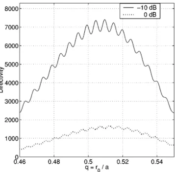
Only an infinite paraboloid generates a plane wave, if the point feed is placed at the GO focus: r0/a⫽0.5. In any finite-size geometry a focal shift occurs, predicted by GO,18 and studied in Ref. 19 by using PO. However in reality, for a finite d, the dependence of Dtoton q⫽r0/a has an even more complex and oscillatory nature. In Fig. 3 is presented the hard ‘‘shallow’’ reflector under two edge illuminations: ⫺10 dB 共the same for all q, solid curve兲 and 0 dB 共omnidi-rectional source, dashed curve兲. In the former case, the pa-rameter kb was slightly varied around the value 8.2 to pro-vide a constant illumination level. One may clearly see that there is not a single, but several positions of the feed provid-ing almost equally good directivity. The broad maximum corresponds to the focal shift predicted by GO:19 it is be-tween r0/a⫽0.5 and r0/a⫽sec␪0/2, that is r0/a⫽ 0.518

FIG. 2. Normalized computation error as a function of the matrix truncation

number, for a hard-surface reflector␪0⫽30°. FIG. 3. Directivity of a hard-surface ‘‘shallow’’ reflector as a function of

the normalized feed position. Solid curve is for the edge illumination⫺10 dB, dashed curve is for nondirective source (kb⫽0). Reflector parameters are: d⫽50␭, f /d⫽0.97 (ka⫽606.9,␪0⫽15°).

here. The period of the smaller oscillations is equal to␭/2. This feature of the near field is clearly not of GO nature, and does not appear to be predicted by high-frequency asymptotic approximations. In Fig. 4, we present total far field radiation patterns, computed for three different edge illuminations. Note that reduction of the edge illumination levels from⫺5 dB to ⫺10 dB 共that is, increasing the beam-width parameter kb, from 4 to 8.4兲 mainly affects the far sidelobes, between 30° and 90°. The feed position here cor-responds to the optimum.

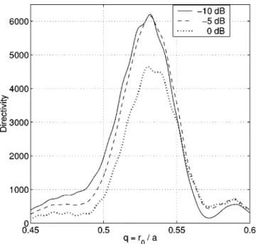
The next series of results illustrates features of the ‘‘deep’’ reflector. In this case, the spherical shape of the latter has a greater effect. The directivity dependence on the feed position共Fig. 5兲 shows a broad maximum in the middle

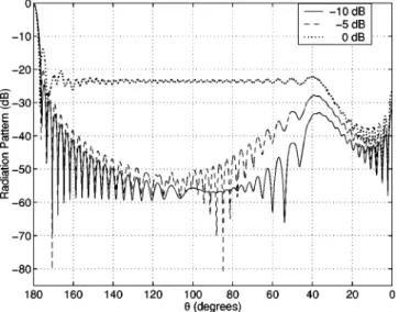
of GO-predicted interval, between r₀/a⫽0.5 and 0.578, but no oscillations. Note that the maximum directivity for the omnidirectional feed is double that of the ‘‘shallow’’ reflec-tor case 共compare with Fig. 3兲, due to doubling the area of reflector. However, the directivity in this case is much more critically dependent on the feed position, the GO focus being completely unacceptable. Far field patterns presented in Fig. 6 are more sensitive to the decrease of edge illumination levels from ⫺5 dB to ⫺10 dB 共by increasing the beam-width parameter kb, from 0.8 to 2.1兲, and show the effect of spherical aberrations, not visible in Fig. 4.

Most of these features are observed for the soft reflectors as well: see Figs. 7 and 8. Similarly for the hard reflector,

FIG. 4. Normalized far field radiation patterns of the same ‘‘shallow’’ re-flector as in Fig. 3, for the feed position r0/a⫽0.507. Edge illuminations

are:⫺10 dB 共solid curve兲, ⫺5 dB 共dashed curve兲, and non-directive source

共dotted curve兲.

FIG. 5. Directivity of a hard-surface ‘‘deep’’ reflector as a function of the normalized feed position. Edge illuminations are: ⫺10 dB 共solid curve兲,

⫺5 dB 共dashed curve兲, and nondirective source 共dotted curve兲. Reflector

parameters are: d⫽50␭, f /d⫽0.5 (ka⫽314.2,␪0⫽30°).

FIG. 6. Normalized far field radiation patterns of the same ‘‘deep’’ reflector as in Fig. 5, for the feed position r0/a⫽0.526. Edge illuminations are:

⫺10 dB 共solid curve兲, ⫺5 dB 共dashed curve兲, and nondirective source 共dotted curve兲.

FIG. 7. Directivity of a soft-surface ‘‘shallow’’ reflector as a function of the normalized feed position. Edge illuminations are:⫺10 dB 共solid curve兲, and nondirective source共dotted curve兲. Reflector parameters are: d⫽20␭, f /d

decreasing the edge illumination below ⫺5 dB has a small effect on the overall directivity. As expected, a soft-surface edge produces smaller sidelobes than a hard-surface one. V. CONCLUSIONS

We have presented a simple but powerful algorithm for the analysis of spherical reflector antennas fed by a scalar beam. It is based on the exact analytical inversion of the singular part of the corresponding full-wave integral equa-tion. This is achieved through the conversion of the problem to dual series equations, and followed by the Abel integral transform to invert the static part 共in the soft case兲, or the ‘‘main’’ part共in the hard case兲. The resulting infinite matrix equations are of Fredholm second kind, thus ensuring exis-tence of the exact solution, and the opportunity of obtaining it within machine precision, by taking more and more equa-tions. This approach was previously used in plane-wave scat-tering analysis; here, it is combined with a complex source-point simulation of a directive feed field employing a function which is an exact solution to the Helmholtz equa-tion. The analytical regularization approach described above can be considered numerically exact because the achievable accuracy is limited only by the computer used, and is uni-form with respect to the frequency and the other parameters. Accurate numerical analysis of the considered problem reveals several interesting features of the wave field that do not seem to be predicted by asymptotic techniques. For ex-ample, besides the well-known focal shift toward the reflec-tor, the directivity 共as a function of the feed position兲 dis-plays not a single, but several, local maxima near the GO-predicted shifted focal point. Generally, optimization of antenna geometry depends on the cost functional. Maximum

directivity is a possible choice of cost functional, but mini-mum sidelobe level is another, or a combination of both is also reasonable. Potential applications of the analysis pre-sented are in the area of hydro-acoustic antenna design.

One possible extension of this analysis is to parabolic or other nonspherical reflectors. Here, an IE, similar to Eq.共5兲 or 共14兲, will require a modified domain of integration. How-ever, analytical regularization of this IE can be based upon the extraction and inversion of the singular static part of the spherical dish IE operator. Hence, the technique presented above will be at the core of the modified analysis.

ACKNOWLEDGMENTS

The first two authors are grateful to NATO and the Royal Society for a research fellowship which supported this work, and also to the Department of Mathematics, University of Dundee, for its support for this work.

1

J. D. Kraus, Antennas共McGraw-Hill, New York, 1988兲.

2_{C. Scott, Modern Methods of Reflector Antenna Analysis and Design}

共Artech House, Boston, 1990兲.

3_{D. C. Jenn, M. A. Morgan, and R. J. Pogorzelski, ‘‘Characteristics of}

approximate numerical modeling techniques applied to resonance-sized reflectors,’’ Electromagnetics 15, 41–53共1995兲.

4_{M. R. Barclay and W. V. T. Rusch, ‘‘ Moment-method analysis of large,}

axially symmetric reflector antennas using entire-domain functions,’’ IEEE Trans. Antennas Propag. 39, 491–496共1991兲.

5

G. A. Deschamps, ‘‘Gaussian beam as a bundle of complex rays,’’ Elec-tron. Lett. 7, 684–685共1971兲.

6_{L. B. Felsen, ‘‘Complex-point source solutions of the field equations and}

their relation to the propagation and scattering of Gaussian beams,’’ Symp. Math. Instituta di Alta Matematica 18, 39–56共1975兲.

7

P. A. Belanger and M. Couture, ‘‘Boundary diffraction of an inhomoge-neous wave,’’ J. Opt. Soc. Am. 73, 446–450共1983兲.

8_{G. A. Suedan and E. V. Jull, ‘‘Scalar beam diffraction by a wide circular}

aperture,’’ J. Opt. Soc. Am. A 5, 1629–1634共1988兲.

9

A. N. Norris, ‘‘ Complex point-source representation of real point sources and the Gaussian beam summation method,’’ J. Opt. Soc. Am. A 3, 2005– 2010共1986兲.

10_{A. N. Norris and T. B. Hansen, ‘‘Exact complex source representations of}

time-harmonic radiation,’’ Wave Motion 25, 127–141共1997兲.

11

T. Ogˇuzer, A. Altintas¸, and A. I. Nosich, ‘‘Accurate simulation of reflector antennas by the complex source—dual series approach,’’ IEEE Trans. Antennas Propag. 43, 793–801共1995兲.

12_{Y. N. Feld and A. K. Ansryan, ‘‘Diffraction of scalar wave by a parabolic}

reflector,’’ Radio Eng. Electron. Phys. 22, 1共1977兲.

13

I. V. Vovk, ‘‘Diffraction of sound waves by a parabolic reflector,’’ Sov. Phys. Acoust. 25, 287–289共1979兲.

14_{S. S. Vinogradov, ‘‘A soft spherical cap in the field of a plane sound}

wave,’’ USSR Comput. Math. Math. Phys. 18, 244–249共1978兲.

15

S. S. Vinogradov, Y. A. Tuchkin, and V. P. Shestopalov, ‘‘Summatory equations with kernels in the form of Jacobi polynomials,’’ Sov. Phys. Dokl. 25, 531–532共1980兲.

16_{D. Colton and R. Kress, Integral Equation Methods in Scattering Theory}

共Wiley-Interscience, New York, 1983兲.

17

M. Abramowitz and I. A. Stegun, Handbook of Mathematical Functions 共Dover, New York, 1965兲.

18_{R. C. Spenser and G. Hyde, ‘‘Studies of the focal region of a spherical}

reflector: Geometrical optics,’’ IEEE Trans. Antennas Propag. AP-16, 317–324共1968兲.

19_{H. Ling, S.-W. Lee, P. T. C. Lam, and W. V. T. Rusch, ‘‘ Focal shifts in}

parabolic reflectors,’’ IEEE Trans. Antennas Propag. AP-33, 744–748 共1985兲.

FIG. 8. Normalized far field radiation patterns of the same reflector as in Fig. 7, for the feed position r0/a⫽0.504. Edge illuminations are: ⫺10 dB

共solid curve兲, ⫺5 dB 共dashed curve兲, and nondirective source 共dotted