1
Testing the Role of Renewable Energy Consumption and Trade Policy on Ecological Footprints of the US: Evidence from Innovative Accounting Tests
Ojonugwa Usman1 and Andrew Adewale Alola2, 3 Samuel Asumadu Sarkodie4
1 Department of Economics, Faculty of Business and Economics,
Eastern Mediterranean University, Famagusta North Cyprus, via Mersin 10, Turkey.
2 Department of Economics and Finance, Faculty of Business and Economics, Istanbul
Gelisim University, Turkey.
3 Department of Financial Technologies, South Ural State University, Chelyabinsk, Russia 4 Nord University Business School (HHN), Post Box 1490, 8049, Bodø, Norway
___________________________________________________________________________
Abstract: Renewable energy technologies are promising, yet, very little is known about its role
as a limiting factor in fossil fuel-attributable environmental degradation — especially in high-income countries. This study investigated the dynamic effect of renewable energy consumption, economic growth, and biocapacity and trade policy on environmental degradation in the United States from 1985Q1 to 2014Q4. To achieve this objective, the study applied an autoregressive distributed lag (ARDL) model to obtain the long-run and short-run dynamic coefficients. Toda-Yamamoto causality test was used to examine the direction of causality while Cholesky decomposition test was for innovative accounting to validate the estimated models. The empirical results divulged that a decline in environmental degradation can be attributed to an increase in renewable energy consumption through its negative effects on ecological footprint. Economic growth and biocapacity were found to exert upward pressure on ecological footprint; however, trade policy exerts downward pressure on ecological footprint. A two-sided causal relationship was established between economic growth and ecological footprint as well as economic growth and biocapacity. In contrast, a one-way causality was confirmed running from trade policy to renewable energy consumption and from renewable energy consumption to biocapacity. The innovative accounting revealed that 14.79% and 8.41% of renewable energy consumption and trade policy caused 0.60% and 9.88% deterioration in the environment. Hence, country-specific energy policies that increase the share of renewable energy in the energy portfolio are recommended.
Keywords: Ecological footprints; renewable energy consumption; Trade policy; Innovative
Accounting tests
2
1. Introduction
In the last decades, environmentalists and environmental stakeholders are increasingly overwhelmed with the impact of environmental degradation and ecological distortions of the globe’s geographical space. The continued and somewhat unwanted climatic experiences, in most cases, resulting into environmental disasters are the common indications that suggest these drastic ‘revolution’ in the earth’s climatic systems. With the increasing human activities, which include the direct and indirect activities on the atmospheric strata and the biosphere, humans’ sustainability has increasingly been endangered. (Alola, 2019; Bekun et al., 2019). For several decades, the impact of human engagements on the environment has consistently been measured by the environmental response to economic growth, population dynamics, energy usage, and several other notable factors (Sarkodie and Owusu, 2016; Emir and Bekun, 2018; Sarkodie, 2018; Sarkodie and Strezov, 2018; Shahbaz and Sinha, 2019; Wang and Dong, 2019). In fact, such environmental impact has consistently been accounted for by emissions from carbon dioxide (CO2). Specifically, the emissions from CO2 is largely believed to
constitute about 76% and 94% of the total United States (US)’ anthropogenic greenhouse gas (GHG) and the anthropogenic CO2 emissions (Energy Information Administration, 2017).
In recent times, and following the ecological accounting vis-a-vis the ecological footprint that was put forward by Wackernagel and Rees (1998), environmental wellbeing and distortions have been examined by using the ecological footprints. This is because the ecological footprint measures the capacity of the earth resources that is available for use or already been expanded by human engagements (Global Footprint Network, 2019). On one hand, the Global Footprint Network (GFN) presents biocapacity as the earth surface’s capacity to produce the human basic ecological needs or resources from the fishing grounds, cropland, grazing land, built-up land, and forest area excluding carbon emissions’ absorption from land surface. In response, the perpetual demand on the ecological products (assets) is increasingly depleted especially in large states, thus accounting for the low or ecological deficit in some countries. Hence, ecological deficit (when the population’s demand on nature is more than the productive capacity of a nature) posits a severe environmental quality and sustainability concerns.
Specifically, the US is currently known to be ecologically deficit (Global Footprint Network, 2019). Although the ecosystem is expected to be managed such that it naturally adjusts and continuously change conditions in a sustainable pattern, the ecological accounting for the US otherwise suggests a serious concern. In previous studies, especially for the US, economic
3
expansion, vast energy (non-renewable fuels) consumption, and population growth are among the factors adjudged to be responsible (Boyce, 1994; Soytas et al., 2007; Shahbaz et al. 2017). However, the recent trade policy of the current US government has potentially continued to create more research questions especially as it relates to both economic and environmental sustainability of the country. With the changes in the US’s trade protocol like the North American Free Trade Agreement (NAFTA) and the introduction of trade embargoes on trade partners, the dynamics of environmental quality would potentially be undermined. For instance, in limiting its trade with China, it suggests that more of the previously imported goods would be produced domestically, thus increasing economic activities. In addition to the dynamics of the country’s trade policy, the surge in the consumption of renewable energy in the US (18% of power mix) is another factor that has continued to compound the demand on its ecological footprints. Importantly, the dynamics of the aforementioned factors is also not unconnected with the degradation of the country’s biocapacity.
Based on the above motivations, this study is aimed at investigating the dynamic impact of renewable energy consumption, economic growth, biocapacity and trade policy on the ecological footprints in the US. In conducting this investigation, quarterly dataset from 1985Q1 to 2014Q4 is employed, thus presenting diverse novelty to extant literature. At first, the study further draws the attention of environmentalists and scholars to the dire environmental concern for the US. In this case, the ecological footprint is employed as against the regular indicator (CO2) which potentially reveals more information on the ecological imbalance of the US. In
addition to the recent study of Alola (2019), this current study investigates which variables among the combinations of the renewable energy consumption, GDP, biocapacity and trade policy exert upward or downward pressure on ecological footprints in the US.
The other part of the study is ordered as follows. Section 2 presents an overview of ecological accounting vis-à-vis ecological footprint and biocapacity. Section 3 covers the material and empirical methodologies. The empirical findings and discussion are reported in Section 4. In section 5, the concluding remarks and policy implication of the study are provided.
2. Environmental quality and sustainability: A synopsis
Since the study of Wackernagel and Rees (1998) on the necessity of reducing the human impact of the environment, the use of ecological footprint has continued to be the toast of
4
environmentalist. For some reasons, the ecological footprint has been recently used as proxy for environmental quality. In a recent study and while investigating the role of economic growth on environmental degradation in the newly industrialized countries, Destek and Sarkodie (2019) affirmed the validity of the environmental Kuznets curve (EKC) hypothesis. Commenting further on the study, ecological footprint is being used in lieu of the conventional CO2 as proxy for environmental quality to obviously evaluate the positive of the EKC.
Although other factors like the energy consumption, financial development were incorporated along with the Gross Domestic Product (GDP), the study found an inverted U-shaped relationship between GDP and the ecological footprint in the selected eleven newly developed countries. Similarly, Al-Mulali et al., (2015) utilized the ecological footprint in place of environmental degradation to investigate the positive of EKC for 93 countries. In this case, the validity of the EKC hypothesis is found to increase with the GDP growth, thus indicting the low and lower middle-income countries are at severe risk of environmental damage. The implication suggested by the study is that the low income countries are not likely equipped with technologies that improve energy efficiency, energy saving and renewable energy, thus experiencing slower economic growth (lower GDP growth).
Furthermore, in addition to investigating the nexus of economic development or income (GDP growth), trade openness, energy consumption and financial development with the ecological footprint, other indicators have recently been employed. For instance, the disaggregated economic activities that include tourism, food and transportation have also been found to exhibit significant relationship with ecological footprint (Gössling et al., 2002; Ozturk et al. 2016; Baabou et al., 2017). While the nexus of the ecological footprint and the tourism industry’s sustainability is being investigated by Seychelles by Gössling et al. (2002), a similar study has been presented for 144 countries by Ozturk et al. (2016). The results found negative connection of the ecological footprint and the GDP growth from tourism, consumption of energy, openness to trade as well as urbanization.; hence it is reaffirmed the hypothesis of EKC holds, which is mostly exist around the upper middle- and high-income countries. Moreover, Baabou et al (2017) found that the drivers of EKC hypothesis in 19 Coastal Mediterranean Cities (CMC) are food consumption, transportation and consumption of manufactured goods. In addition, Baabou et al., (2017) noted empirically that the differences in the ecological footprint of the cities are potentially associated with socio-economic factors that include the disposable income, infrastructure, and cultural habits.
5
Moreover, in identifying the important of sustainable development of the regional ecology and economic system of China, Yue (2011) utilized the spatial analysis to examine the supply and demand of biocapacity across the country’s North-western region. Subsequently, the study revealed the following impacts of spatial heterogeneity on the biocapacity supply of the Northwestern region. Firstly, it affirmed a decline in the biocapacity supply from the eastern region to the middle, and then a rise from the middle to the west is however observed. Secondly, ecological deficit in the provincial and county levels are observed to be larger notwithstanding small regional ecological deficit resulting from the gap between the biocapacity demand and supply in the region. Lastly, it suggested that biocapacity supply is also determined by population density and the intensity of human exploitations. Additionally, Liu et al., (2011) and Kissinger and Rees (2010) are among the studies that have revealed the nexus of ecological capacity and different human activities in China and the US respectively. While Liu et al. (2011) hinted on the imbalance of the demand-supply ecological carrying capacity across China, the impact of the US’s imports of renewable resources on the ecosystem area is examined by Kissinger and Rees (2010).
3. Materials and data
3.1 Data
We use quarterly data from 1985Q1 to 2014Q4 to investigate the dynamic effects of renewable energy and trade policy on environmental quality and environmental sustainability in the US. To achieve this objective, use is made of the variables such as renewable energy, trade policy, gross domestic product (GDP) per capita, ecological footprint per capita, and biocapacity (gha/person). Environmental quality is proxied by ecological footprint (gha/person) while biocapacity is a proxy for environmental sustainability. Renewable energy is the amount of renewables to total supply of primary energy. GDP is a proxy for economic growth while trade policy is specifically used following the recent paper by Alola (2019) as a proxy for uncertainty in the US trade policy. With the aim of stabilizing the variance, we take the natural logarithms of all the variables.
3.2 Model estimations and procedures
In this study, we aim at investigating the effects of renewable energy and trade policy on environmental quality and environmental sustainability. Therefore, incorporating control variable, which include economic growth, we specify our equations as follows:
6
0 1 2 3 4
lnHFPt lnRE lnGDP lnBIOCAP lnTPt (1)
where 0 is the constant and t is the independently and identically distributed stochastic term. lnHFP is the log of ecological footprint, lnREis the log of renewable energy consumption, lnTP is the log of trade policy measure, lnGDP is the log of the economic growth (GDP per capita) and lnBIOCAP is the log of biocapacity. Equation (1) is concerned with measuring the effects of the fundamental variables on environmental degradation. To this extent, we applied Autoregressive Distributed Lag (ARDL) model proposed by Pesaran et al., (2001) using Equations (1). The transformed of these equations to unrestricted error correction model (UECM) are stated as follows:
2 0 1 1 2 1 3 1 4 1 5 1 lnHFTt lnHFPt lnREt lnGDPt lnBIOCAPt lnTPt 1 2 3 4 1 1 2 1 3 1 4 1 0 0 0 0 lnHFP lnRE lnGDP lnBIOCAP p q q q t t t t i i i i
5 5 1 0 lnTP q t t i
(2)where is the natural logarithm of each of the variables captured in the model, Δ is the difference operator. The first section of equation (2) is aptly used to obtain the long-run coefficients of the HFP equation, while the second section is used to obtain the short-run coefficients.
It could be noted that the ecological footprints, a measure of environmental degradation may be not change to the path of long-run equilibrium if there is a shock to any of the independent variables. The speed at which ecological footprints adjusts from short-run to long-run equilibrium level is captured by the estimated error correction model (ECM) equation as follows: 2 0 1 1 2 1 3 1 4 1 5 1 lnHFTt lnHFPt lnREt lnGDPt lnBIOCAPt lnTPt 1 2 3 4 1 1 2 1 3 1 4 1 0 0 0 0 lnHFP lnRE lnGDP lnBIOCAP p q q q t t t t i i i i
5 5 1 1 0 lnTP q t t t i ecm
(3) ln7
where all the variables remained as defined in equation (2). ecmt1 is the lag of the residuals. Using the methodology of ARDL bounds testing, we can estimate our models whether the variables are I(0) , I(1) or integrated fractionally. In addition, the model performs better compared to other cointegration tests in a small sample size. Therefore, we carry out a coingration test using Pesaran et al. (2001) approach of bounds test as well as the critical values of Kripfganz and Schneider (2018), which are perhaps approximately p-values test results. The null hypothesis of the test is that 1 2 3 4 5 0 and the alternative is that
1 2 3 4 5 0
. Before estimation of the model, we test the stationarity properties of the series explored through the Augmented Dickey-Fuller (ADF) and Phillips-Perron (PP). The null hypothesis for these tests states that H0: 0. This is tested against the alternative of H0: 0.
3.3 Causality test
For better understanding of the causal interaction between variables, which are essential for crafting energy and environmental policies for development sustainability, we therefore apply Toda-Yamamoto conditional Granger causality test. This test aptly examines causality direction of the variables using a modified WALD Statistic. The test has several advantages over the Pairwise Granger causality approach, which assumes that the variables are indeed stationary at I(0). Should in case the variables are stationary at I(0) and I(1), Toda-Yamamoto can be conveniently applied and produce robust results. According to Toda and Yamamoto (1995), this test is implemented on the framework of Autoregressive Distributed Lag (VAR) model with the null hypothesis, which clearly states that
H :
0
120
i.4. Empirical Results
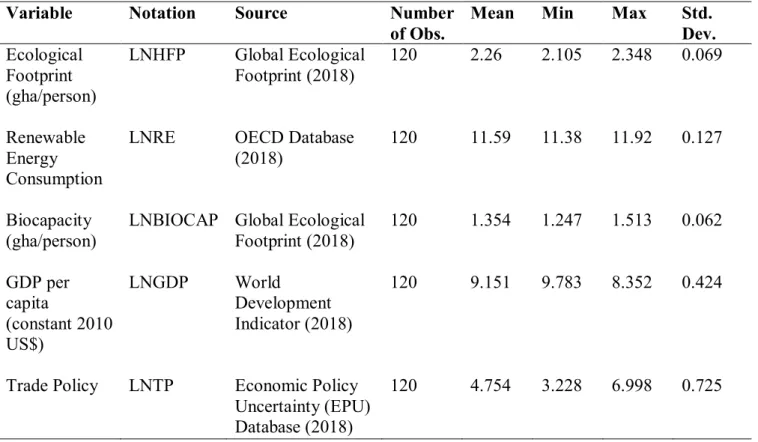
Table 1 discloses the summary of these variables, their measurements, and sources as well as the statistical characteristics. The result show that the highest mean score of variables is owned by renewable energy consumption with about 11.59 while biocapacity has the lowest. The result further displays that all the variables tend to be less volatile. Furthermore, Table 2 discloses the results of the pair-wise correlations. We find a negative correlation between ecological footprint and fundamental variables such as consumption of renewable energy, GDP, and trade policy while a positive correlation between ecological footprint and biocapacity. We equally find a positive correlation between consumption of renewable energy and GDP as well as renewable
8
energy consumption and trade policy. The correlation between GDP and biocapacity is negative while GDP and trade policy is positive. Finally, the correlation between biocapacity and trade policy is negative. The correlations between the variables are all statistically significant at 1% significance level.
Table 1: Summary Descriptive statistics
Variable Notation Source Number
of Obs.
Mean Min Max Std.
Dev. Ecological Footprint (gha/person) LNHFP Global Ecological Footprint (2018) 120 2.26 2.105 2.348 0.069 Renewable Energy Consumption
LNRE OECD Database (2018)
120 11.59 11.38 11.92 0.127
Biocapacity (gha/person)
LNBIOCAP Global Ecological Footprint (2018) 120 1.354 1.247 1.513 0.062 GDP per capita (constant 2010 US$) LNGDP World Development Indicator (2018) 120 9.151 9.783 8.352 0.424
Trade Policy LNTP Economic Policy Uncertainty (EPU) Database (2018)
120 4.754 3.228 6.998 0.725
Source: Authors’ computation
Table 2: Pairwise Correlations
Variable LNHFT LNRE LNGDP LNBIOCAP LNTP
LNHFP 1.000000 --- LNRE -0.888832 1.000000 (-21.070) --- LNGDP -0.567155 0.635684 1.000000 (-7.4803) (8.9453) --- LNBIOCAP 0.547055 -0.611425 -0.897010 1.000000 (7.0981) (-8.3935) (-22.045) --- LNTP -0.603883 0.628068 0.581310 -0.606881 1.000000
9
(-8.2299) (8.7676) (7.7606) (-8.2945) ---
Notes: The values in the parenthesis are the t-statistic.
2.10 2.15 2.20 2.25 2.30 2.35 2.40 1985 1990 1995 2000 2005 2010 LNHFP 11.3 11.4 11.5 11.6 11.7 11.8 11.9 12.0 1985 1990 1995 2000 2005 2010 LNRE 8.0 8.4 8.8 9.2 9.6 10.0 1985 1990 1995 2000 2005 2010 LNGDP 1.24 1.28 1.32 1.36 1.40 1.44 1.48 1.52 1985 1990 1995 2000 2005 2010 LNBIOCAP 3 4 5 6 7 8 1985 1990 1995 2000 2005 2010 LNTP
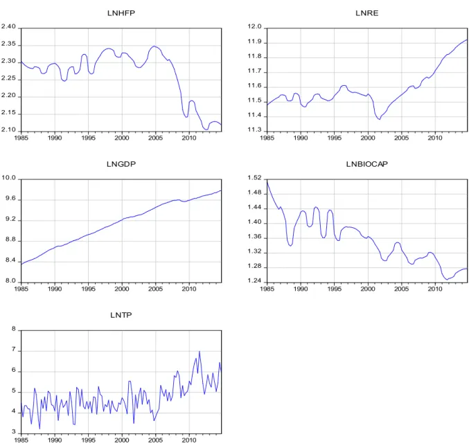
Figure 1: Time plots of log of ecological footprints, renewable energy consumption, GDP, biocapacity and trade policy
The time plots of the log of ecological footprints, renewable energy consumption, output growth measured by GDP, biocapacity, and trade policy are dislosed in Figure 1. Based on this figure, it is found that there is no clear-cut evidence of trade in all the variables except output growth measure. We also observe that the variables are all characterized by fluctuations except in the case of GDP which trends upward. The fluctuations observed is more conspicuous in the trade policy variables.
10
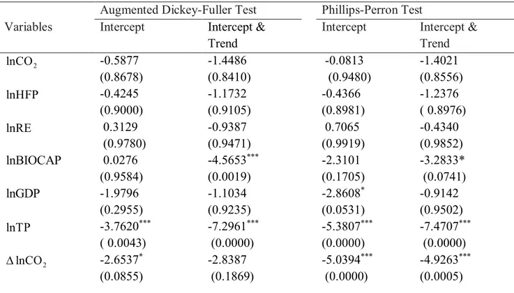
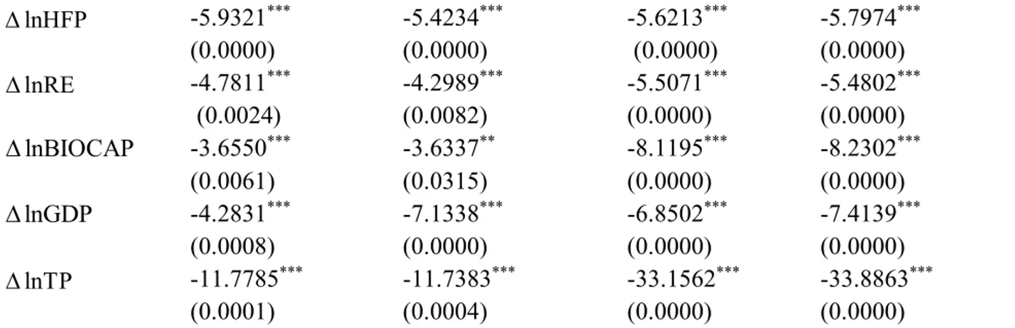
We further test for the stationarity properties of the series so that we can apply the appropriate methodology. Our results based on the ADF test by Dickey and Fuller (1979) and the PP test by Phillips and Perron (1988) (See Table 3), indicate that the variables are all integrated of order one, I(1) except trade policy and biocapacity which are I(0). Therefore, we move to the next stage by establishing the relationship among the investigated variables. This test is performed using the ARDL bounds testing framework. We consider that the ARDL bounds testing approach to cointegration is most appropriate since we have mixed order of integration (See Pesaran et al. 2001). Therefore, the bounds test cointegration applied in this study is based on the unrestricted constant and no Trend. The test uses Akaike Information Criteria (AIC) lag length selection. The results as displayed in Table 4 show that the null hypothesis of no long-run relationship on the basis of F-statistic and t-statistic is rejected at the significance test of 1%. In other words, a well-established long-run relationship among the variables has been observed. Furthermore, for the purpose of robustness, we applied the Pesaran et al. (2001) bounds testing cointegration using Kripfganz and Scheneider (2018) critical values and approximate p-values. The results as shown in Table 5 indicate that the null hypothesis of no cointegration is rejected based on the significance of probability values at lower bound and upper bound. Hence, we proceed to estimate our models specified in equations (2) and (3)
Table 3: ADF and PP Unit Root Tests
Augmented Dickey-Fuller Test Phillips-Perron Test
Variables Intercept Intercept &
Trend
Intercept Intercept &
Trend 2 lnCO -0.5877 (0.8678) -1.4486 (0.8410) -0.0813 (0.9480) -1.4021 (0.8556) lnHFP -0.4245 (0.9000) -1.1732 (0.9105) -0.4366 (0.8981) -1.2376 ( 0.8976) lnRE lnBIOCAP 0.3129 (0.9780) 0.0276 (0.9584) -0.9387 (0.9471) -4.5653*** (0.0019) 0.7065 (0.9919) -2.3101 (0.1705) -0.4340 (0.9852) -3.2833* (0.0741) lnGDP -1.9796 (0.2955) -1.1034 (0.9235) -2.8608* (0.0531) -0.9142 (0.9502) lnTP -3.7620*** ( 0.0043) -7.2961*** (0.0000) -5.3807*** (0.0000) -7.4707*** (0.0000) 2 lnCO -2.6537* (0.0855) -2.8387 (0.1869) -5.0394*** (0.0000) -4.9263*** (0.0005)
11 lnHFP -5.9321*** (0.0000) -5.4234*** (0.0000) -5.6213*** (0.0000) -5.7974*** (0.0000) lnRE -4.7811*** (0.0024) -4.2989*** (0.0082) -5.5071*** (0.0000) -5.4802*** (0.0000) lnBIOCAP -3.6550*** (0.0061) -3.6337** (0.0315) -8.1195*** (0.0000) -8.2302*** (0.0000) lnGDP -4.2831*** (0.0008) -7.1338*** (0.0000) -6.8502*** (0.0000) -7.4139*** (0.0000) lnTP -11.7785*** (0.0001) -11.7383*** (0.0004) -33.1562*** (0.0000) -33.8863*** (0.0000) Notes: ***, ** and * denote significance level at 1%, 5%, 10% levels.
Table 4: Pesaran et al. (2001) bounds testing cointegration analysis
Models Statistics K
lnHFPf(lnRE, lnGDP, lnBIOCAP, lnTP) F-Stat: 6.8486*** 4 t-Stat: -5.4039***
Critical Value Bound Tests Lower I(0) Upper I(1)
F-Statistic at 1 Percent t-Statistic at 1 Percent 3.74 -2.548 5.06 -3.644 Notes: *** denote significance level at 1%.
Table 5: Pesaran et al. (2001) bounds testing cointegration using Kripfganz and Scheneider (2018) critical values and approximate p-values
K=4 10% 5% 1% P-value
I(0) I(1) I(0) I(1) I(0) I(1) I(0) I(1)
F-crit. 2.458 3.601 2.904 4.147 3.889 5.327 0.000 0.001 t-crit. -2.530 -3.614 -2.844 -3.964 -3.457 -4.631 0.000 0.001 F-cal. 6.752
t-cal. -5.367
Notes: F-crit. and t-crit. represent the critical values for F-statistic and t-statistic while F-cal. and t-call represent the values of F-calculated and t-calculated.
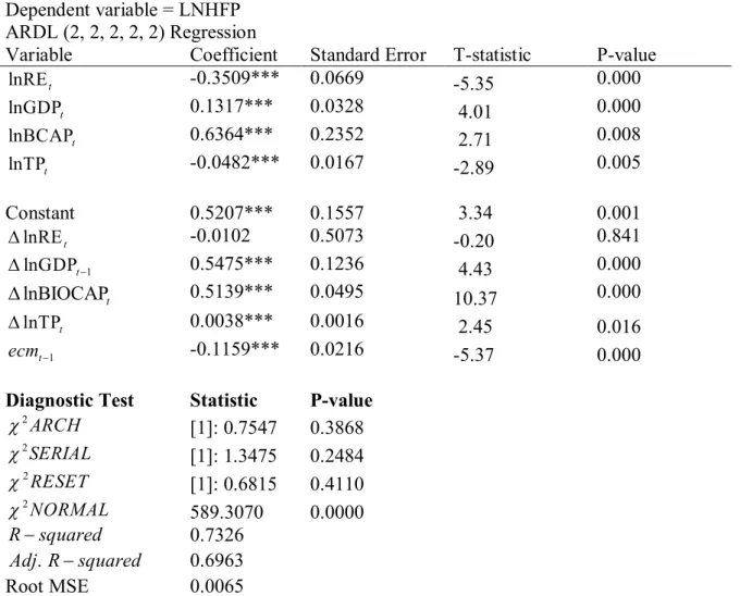
Table 6 clearly discloses the estimates of the long run and short run environmental degradation functions. According to the long-run results, a 1% increase in renewable energy consumption and trade policy causes ecological footprints to decline by 0.3508% and 0.0482%, while a 1% increase in GDP and biocapacity increases ecological footprints by 0.1317% and 0.6364%. Similarly, in the short run, the coefficient of the renewable energy consumption is negatively related to ecological footprints but there is no evidence that it is statistically significant.
12
However, a 1% increase in GDP, biocapacity and trade policy increases ecological footprints by 0.5475%, 0.5139% and 0.0038% respectively.
The negative relationship between renewable energy consumption and ecological footprints in the long run indicates that renewable energy consumption reduces environmental degradation through its negative effect on ecological footprints. In other words, the results suggest that renewable energy consumption in the US is improving environmental quality as per the results of this study. Therefore, our results are aligned with Apergis and Payne (2009), Shahbaz et al. (2013), Ben Jebli and Ben Youssef (2016). On the contrary, our findings do not agree with Apergis et al. (2010), Ben Jebli et al. (2015) Ben Jebli and Ben Youssef (2017) who argued that renewables are positively related to environmental degradation. Furthermore, the results of the short run indicate that, even though the coefficient is negative, it is statistically insignificant. The reason can be traceable to the combustible renewables and waste in the renewable energy consumption data explored; though this variable is adjudged to emit less pollution compared to the fossil fuel energy consumption or non-renewable energy consumption
The result of the positive connection between GDP and ecological footprint indicates that GDP is a major source of environmental degradation in the US. This is due to the intensive use of fossil energy required by the firms for production process. As GDP increases, more pressure is mounted on ecological footprints components such as fishing grounds, cropland, grazing land, built-up land, forest area, and the carbon emissions’ absorption from land surface. This subsequently lead to environmental damage (Al-Mulali et al. 2015; Rafindadi, 2016; Ranfindadi and Ozturk, 2017; Shahbaz et al. 2017; Usman et al. 2019). More so, the adverse effect of trade policy on ecological footprint in the long run suggests that as trade policy in the US encourages trade with other countries, the pressure on biocapacity and ecological footprint reduces. This is because, the costs required for the production of goods and services in the countries of most trading partners such as China and North American countries such as Mexico, Brazil, as well as African countries are lower compared to the US. The implication for this result is that environmental quality improves through the negative effect of trade policy on ecological footprints of the US. However, in the short run, the opposite is the order of the day.
We conducted some diagnostic tests on the model estimation. The results of these tests reveal that there is no evidence of serial correction and heteroscedasticity. More so, while the
13
functional form of the model is perhaps correctly identified but there is no evidence to support the normal distribution of the residual. Finally, the stability of the model is being checked through CUSUM and CUSUM squared. The results obviously indicate stability of the model at the 5% level of significance.
Table 6: Long-run ARDL Coefficients Dependent variable = LNHFP
ARDL (2, 2, 2, 2, 2) Regression
Variable Coefficient Standard Error T-statistic P-value
lnREt -0.3509*** 0.0669 -5.35 0.000 lnGDPt 0.1317*** 0.0328 4.01 0.000 lnBCAPt 0.6364*** 0.2352 2.71 0.008 lnTPt -0.0482*** 0.0167 -2.89 0.005 Constant 0.5207*** 0.1557 3.34 0.001 lnREt -0.0102 0.5073 -0.20 0.841 1 lnGDPt 0.5475*** 0.1236 4.43 0.000 lnBIOCAPt 0.5139*** 0.0495 10.37 0.000 lnTPt 0.0038*** 0.0016 2.45 0.016 1 t ecm -0.1159*** 0.0216 -5.37 0.000
Diagnostic Test Statistic P-value
2 ARCH [1]: 0.7547 0.3868 2 SERIAL [1]: 1.3475 0.2484 2 RESET [1]: 0.6815 0.4110 2 NORMAL 589.3070 0.0000 Rsquared 0.7326 . Adj Rsquared 0.6963 Root MSE 0.0065
Notes: ***, ** and * denote rejection of the null hypothesis at 1% , 5% and 10% level of significance. The lag length selected using Akaike Information Criteria (AIC) 6.SERIAL2 ,ARCH2 , RESET2 and NORMAL2 denote are tests for serial-correlation, heteroscedasticity, functional as well as normality test. [ ] represents the optimal lag selection for diagnostic tests; the case 3:Unrestricted Constant and No Trend is used.
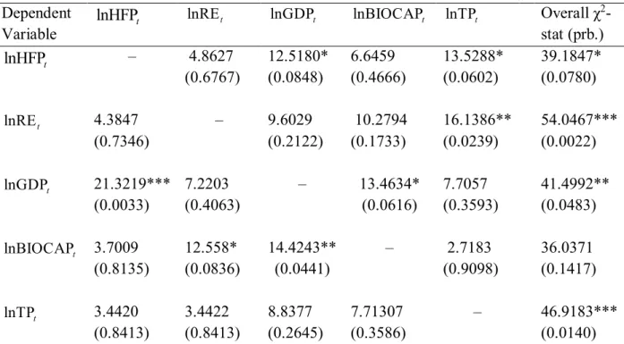
Table 7 presents the results of the Toda-Yamamoto causality test. The results show that there is a two-sided causal relationship between GDP and ecological footprints as well as GDP and biocapacity. The results further show that a one-way causal relationship runs from trade policy to ecological footprints and from trade policy to renewable energy consumption. In addition, renewable energy consumption Granger-cause biocapacity while there is no evidence that any of the variables captured Granger-cause trade policy. These results are supported by Apergis
14
and Payne (2010, 2011), Chang et al. (2013), Lin and Moubarak (2014), Al-Mulali et al. (2015), Kahia et al. (2016), Ben Jebli and Ben Youssef (2017), Destek and Sarkodie (2019). Furthermore, the causal relationship running GDP to ecological footprints supports the hypothesis of growth-led pollutant emissions which has been established in the literature (See Usman et al. 2019; Bekun et al. 2019).
Table 7: Toda-Yomamoto Causality Test for Environmental Degradation Dependent
Variable
lnHFPt lnREt lnGDPt lnBIOCAPt lnTPt Overall χ2 -stat (prb.) lnHFPt – 4.8627 (0.6767) 12.5180* (0.0848) 6.6459 (0.4666) 13.5288* (0.0602) 39.1847* (0.0780) lnREt 4.3847 (0.7346) – 9.6029 (0.2122) 10.2794 (0.1733) 16.1386** (0.0239) 54.0467*** (0.0022) lnGDPt 21.3219*** (0.0033) 7.2203 (0.4063) – 13.4634* (0.0616) 7.7057 (0.3593) 41.4992** (0.0483) lnBIOCAPt 3.7009 (0.8135) 12.558* (0.0836) 14.4243** (0.0441) – 2.7183 (0.9098) 36.0371 (0.1417) lnTPt 3.4420 (0.8413) 3.4422 (0.8413) 8.8377 (0.2645) 7.71307 (0.3586) – 46.9183*** (0.0140) Notes: ***, ** and * denote rejection of the null hypothesis at 1% , 5% and 10% level of significance. The lag length selected using Akaike Information Criteria (AIC) 6+1.
Results of Innovative Accounting Test
In furtherance to the UECM/ARDL bounds testing technique, we use the innovative accounting tests to properly understand the dynamic contribution of each variable to ecological footprints. These tests are the combinations of the error forecast variance decomposition and impulse response functions. Table 8 reveals the analysis of the error forecast variance decomposition using 10 periods ahead of the sample period. Based on the results, the error forecast variance decomposition of the ecological footprint (environmental degradation) attributed to its innovative shock is the largest contributor with 65.1%. This is followed by the contribution of biocapacity with about 10.4% while policy of trade and economic growth contribute about 9.6% and 8.7% to ecological footprints in the US. The last contributor to the ecological footprints is the renewable energy consumption with about 6.3%.
15
Our results further show that the contribution of renewable energy to its own shocks is as high as 81.09%. This is followed by 16.85% following the shocks in ecological footprints. The contribution of GDP, biocapacity and trade policy to the error forecast of renewable energy consumption is as low as 0.60%, 1.00% and 0.46%. Furthermore, the results depict that the contribution of GDP to own shocks is 61.86%, and distantly followed by biocapacity with 14.79%, ecological footprints with 13.23%, trade policy with 8.41% and renewable energy consumption with just 1.71%. In the case of the biocapacity, the results demonstrate that ecological footprint is its major contributor. As shown by the result, ecological footprint contributes about 49.50% to the error forecast decomposition of biocapacity. This is followed by its own shocks with about 43.48% and GDP with about 5.68%. The contribution of renewable energy consumption and trade is just 0.92% and 0.41% respectively. Finally, the error forecast variance decomposition of trade policy due to its innovative shocks is about 84.10%, followed by ecological footprints with about 9.88%, and biocapacity with about 2.92%, while renewable energy and GDP contribute 1.62% and 1.48% to trade policy. The implication for these results is that the variables in the model estimations have bidirectional relationships.
Following these results, the major finding we observe that an increase in renewable energy consumption to improve economic growth causes lower deterioration in the environmental quality while an increase in trade policy to improve growth deteriorates environmental quality drastically. As shown by Table 8, it is unequivocally clear that a 14.79% increase in renewable energy consumption is corresponded with just about 0.60% rise in environmental degradation while a 8.41% increase in trade policy lead to about 9.88% increase in environmental deterioration. These results, therefore, align with our earlier model estimation, which emphatically revealed the importance of renewable energy consumption in the pursuit of economic growth on the basis that it releases less pollution to the environment compared to fossil fuel energies.
The second part of the innovative accounting approach is the impulse response analysis. As disclosed by Figure 2, the response of the ecological footprints to a standard deviation shock to own variable is positive and significant. The results further show that the responses of ecological footprints to a shock in renewable energy consumption, biocapacity and trade policy are all negative. In the case of renewable energy consumption, it is found statistically
16
significant while in the case of trade policy its significance begin from the fifth quarter. Similarly, for biocapacity, it is only found significant between quarter five and seven. Regarding the response of renewable energy to a shock to own variable and other variables, we found interesting results. For example, the response of renewable energy consumption to own shock is positive and statistically significant. The result further displays that renewable energy consumption first responds positively and insignificantly to the shocks in GDP and trade policy. However, for GDP, the response becomes negative after the seventh quarters. In the case of trade policy, the response becomes unnoticeable and consequently negative after the seventh quarters. The response of renewable energy consumption to trade policy is initially negative up to the fifth quarters and crosses to positive thereafter even though the response is insignificant. The empirical result further demonstrates that the response of GDP to a shock in ecological footprint and renewable energy consumption is positive. This response is significant up to the seventh quarters in the case of a shock in ecological footprint while insignificant in the case of renewable energy consumption. The response of GDP to its shocks is positive and statistically significant while the response of GDP to biocapacity and trade policy is negative and statistically significant for biocapacity but in the case of trade policy, the response becomes statistically significant after the fourth quarters.
Our empirical results further divulge that the response of biocapacity to a shock in ecological footprint is positive and statistically significant up to the fifth months and gradually declines until it becomes stabilized in the eighth quarters. For the renewable energy, it is found that the response to its shocks is positive and insignificant. This gradually falls to its steady state after the fourth quarters. The result of the response of GDP to biocapacity is negative and statistically significant up to the ninth quarters, after which it becomes neutral. More so, the response of biocapacity to own shock is positive and significant up to the fifth quarter. This perhaps declines gradually and then hits negative at the ninth quarters. Finally, the response biocapacity to a shock in trade policy is positive and insignificant. This declines gradually to its steady state after the ninth quarters. Similarly, as regards to the response of trade policy to a shock in ecological footprints, we observe it to have a negative and insignificant impact. For renewable energy consumption, the effect is not noticeable in the first three quarters even though it is positive and insignificant. The response of trade to a shock in GDP is negative and moves to its equilibrium after the second quarters. In addition, the result shows that trade policy positively responds to a shock in biocapacity. This becomes negative after the second quarters
17
and then move to it steady state gradually after the sixth quarters, while the response of trade policy to its own shock is positive and gradually decline to become neutral after the third quarters.
Table 8: Innovative Accounting Approach
Variance Decomposition of LNHFP:
Period S.E. LNHFP LNRE LNGDP LNBIOCAP LNTP
1 0.009796 100.0000 0.000000 0.000000 0.000000 0.000000 2 0.016893 97.95296 0.046272 1.692339 0.111747 0.196678 3 0.022700 94.02464 0.211570 3.392090 0.913724 1.457975 4 0.027403 88.74846 0.547173 4.900442 2.480738 3.323188 5 0.031255 83.18550 1.082313 6.161902 4.449336 5.120944 6 0.034471 78.03041 1.819478 7.150976 6.392767 6.606365 7 0.037198 73.63164 2.739255 7.861624 8.018014 7.749467 8 0.039535 70.07540 3.810252 8.317766 9.209122 8.587459 9 0.041557 67.28708 4.995957 8.563321 9.982108 9.171531 10 0.043326 65.12271 6.258070 8.648738 10.41857 9.551917 Variance Decomposition of LNRE:
Period S.E. LNHFP LNRE LNGDP LNBIOCAP LNTP
1 0.012037 0.000000 99.68959 0.310408 0.000000 0.000000 2 0.021659 0.219946 99.24795 0.127491 0.001157 0.403460 3 0.029774 0.476426 98.61033 0.621906 0.039815 0.251524 4 0.036472 0.593657 97.30525 1.841026 0.085723 0.174341 5 0.042001 0.584893 95.44018 3.735793 0.089960 0.149171 6 0.046625 0.509030 93.15334 6.140268 0.073050 0.124313 7 0.050596 0.432271 90.51198 8.839608 0.105154 0.110982 8 0.054124 0.408058 87.56464 11.62589 0.256246 0.145173 9 0.057369 0.465008 84.38689 14.33058 0.559837 0.257683 10 0.060435 0.604734 81.09218 16.83896 1.003697 0.460433 Variance Decomposition of LNGDP:
Period S.E. LNHFP LNRE LNGDP LNBIOCAP LNTP
1 0.005188 5.631263 0.000000 94.24394 0.124793 0.000000 2 0.008285 13.75165 1.292345 84.37146 0.565872 0.018668 3 0.011520 16.46393 3.909010 77.79547 0.975746 0.855846 4 0.014756 16.72182 6.801406 72.80514 1.301494 2.370134 5 0.017913 16.06493 9.330895 69.19627 1.526246 3.881653 6 0.020916 15.23546 11.30444 66.61433 1.663569 5.182198 7 0.023718 14.50182 12.73749 64.76917 1.733831 6.257679 8 0.026298 13.93228 13.72443 63.45297 1.756122 7.134196 9 0.028650 13.51883 14.37479 62.51853 1.745724 7.842123
18
10 0.030786 13.23010 14.78641 61.85999 1.714147 8.409347 Variance Decomposition of LNBIOCAP:
Period S.E. LNHFP LNRE LNGDP LNBIOCAP LNTP
1 0.012183 53.47959 1.256648 0.916672 44.34709 0.000000 2 0.019867 52.68523 1.129229 2.490321 43.69480 0.000418 3 0.024365 51.57713 1.029717 3.623474 43.74944 0.020241 4 0.026519 50.64769 0.960791 4.505179 43.78859 0.097744 5 0.027335 50.05624 0.922409 5.111701 43.69704 0.212615 6 0.027563 49.77014 0.907756 5.459795 43.54602 0.316293 7 0.027608 49.65841 0.906430 5.618301 43.43809 0.378772 8 0.027624 49.60328 0.910333 5.672564 43.41120 0.402618 9 0.027642 49.55287 0.915895 5.685097 43.43966 0.406477 10 0.027659 49.50356 0.922604 5.687217 43.48066 0.405967 Variance Decomposition of LNTP:
Period S.E. LNHFP LNRE LNGDP LNBIOCAP LNTP
1 0.519783 0.720530 0.006664 1.367049 1.934229 95.97153 2 0.540562 2.474262 0.006250 1.503411 1.790483 94.22559 3 0.547921 4.471150 0.032302 1.516549 2.237004 91.74300 4 0.555048 6.327406 0.126109 1.503986 2.639078 89.40342 5 0.560232 7.678328 0.293407 1.486802 2.779966 87.76150 6 0.563711 8.539228 0.518310 1.469952 2.775423 86.69709 7 0.566259 9.069671 0.779782 1.457817 2.752595 85.94013 8 0.568473 9.414272 1.058431 1.455415 2.771070 85.30081 9 0.570634 9.666840 1.340335 1.463786 2.834720 84.69432 10 0.572817 9.881538 1.617903 1.479877 2.922844 84.09784 Cholesky Ordering: LNHFP LNRE LNGDP LNBIOCAP LNTP
19 -.01 .00 .01 2 4 6 8 10 Response of LNHFP to LNHFP -.01 .00 .01 2 4 6 8 10 Response of LNHFP to LNRE -.01 .00 .01 2 4 6 8 10 Response of LNHFP to LNGDP -.01 .00 .01 2 4 6 8 10 Response of LNHFP to LNBIOCAP -.01 .00 .01 2 4 6 8 10 Response of LNHFP to LNTP -.02 -.01 .00 .01 .02 2 4 6 8 10 Response of LNRE to LNHFP -.02 -.01 .00 .01 .02 2 4 6 8 10
Response of LNRE to LNRE
-.02 -.01 .00 .01 .02 2 4 6 8 10 Response of LNRE to LNGDP -.02 -.01 .00 .01 .02 2 4 6 8 10
Response of LNRE to LNBIOCAP
-.02 -.01 .00 .01 .02 2 4 6 8 10 Response of LNRE to LNTP -.005 .000 .005 .010 2 4 6 8 10 Response of LNGDP to LNHFP -.005 .000 .005 .010 2 4 6 8 10 Response of LNGDP to LNRE -.005 .000 .005 .010 2 4 6 8 10 Response of LNGDP to LNGDP -.005 .000 .005 .010 2 4 6 8 10 Response of LNGDP to LNBIOCAP -.005 .000 .005 .010 2 4 6 8 10 Response of LNGDP to LNTP -.005 .000 .005 .010 2 4 6 8 10 Response of LNBIOCAP to LNHFP -.005 .000 .005 .010 2 4 6 8 10
Response of LNBIOCAP to LNRE
-.005 .000 .005 .010 2 4 6 8 10 Response of LNBIOCAP to LNGDP -.005 .000 .005 .010 2 4 6 8 10
Response of LNBIOCAP to LNBIOCAP
-.005 .000 .005 .010 2 4 6 8 10 Response of LNBIOCAP to LNTP .0 .2 .4 2 4 6 8 10 Response of LNTP to LNHFP .0 .2 .4 2 4 6 8 10 Response of LNTP to LNRE .0 .2 .4 2 4 6 8 10 Response of LNTP to LNGDP .0 .2 .4 2 4 6 8 10 Response of LNTP to LNBIOCAP .0 .2 .4 2 4 6 8 10 Response of LNTP to LNTP Response to Cholesky One S.D. (d.f. adjusted) Innovations ± 2 S.E.
Figure 1: Impulse Response Function (IRF) for Environmental Degradation Function.
20
5. Conclusion and policy recommendations
Over the years, the attention of the world has been drawn to the adverse effect of environmental degradation resulting from human activities. In other words, the changes in the natural levels and the distribution of chemical elements as well as their compounds have threatened the well-being of the world. In the US, government has pursued devise of environmental and energy policies such as renewable energy consumption to lessen the consumption of energy from fossil fuels, which cause huge pollutions to the detriment of human health. Given this background, the paper investigates not only the dynamic impact of renewable energy consumption, economic growth, biocapacity and trade policy on the ecological footprint in the US using quarterly dataset from 1985Q1 to 2014Q4. To achieve this objective, we tested the stationarity properties of the variables and their cointegration using ADF and PP unit root tests as well as the bounds testing cointegration technique. The robustness of this cointegration was checked using Kripfganz and Scheneider (2018) critical values and approximate p-values of the original bounds testing cointegration. The results of the ADF and PP showed a mixed order of integration as well as cointegration among the variables. The results of the long-run and the short-run coefficients were obtained from the ARDL bounds testing approach. The results of the long-run showed that a 1% increase in renewable energy consumption and trade policy reduced ecological footprints to decline by 0.3508% and 0.0482%, and by implication increased environmental quality while a 1% increase in GDP and biocapacity increased ecological footprints by 0.1317% and 0.6364% which by implication reduced environmental quality. Similarly, in the short run, the coefficient of the renewable energy consumption is negatively related to ecological footprints but there was no evidence that it was statistically significant. However, a 1% increase in GDP, biocapacity and trade policy increased ecological footprints by 0.5475%, 0.5139% and 0.0038%.
In order to check the causal relationship between the variables, we applied a conditional Granger causality test developed by Toda and Yamamoto (1995). The results of this test showed evidence of a feedback causal effect between GDP and ecological footprints as well as GDP and biocapacity. Also, the results divulged that a one-way causal relationship was evidently running from trade policy to renewable energy consumption and from renewable energy consumption to biocapacity. Complementing the causality test was the accounting innovative tests, which used error forecast variance decompositions and impulse responses. The results of the error forecast variance decomposition showed that apart from the effect of
21
own shocks, the shocks to biocapacity had the highest effect on ecological footprints, followed by trade policy, GDP and lastly renewable energy consumption. However, in terms of driving economic growth with less pollution to the environment, renewable energy consumption stood out. Furthermore, the results based on the impulse response function displayed that the response of the ecological footprint to itself was positive. More so, the responses of ecological footprints to a shock in renewable energy consumption, biocapacity and trade policy are negative while the response of ecological footprints to a shock in GDP was found positive.
Therefore, to reduce environmental degradation and improve environmental quality, the pursuit of pollution-free economic growth and energy mix are essential. Based on the findings of this study, we suggest that more energy policies should encourage huge investments in renewables like nuclear power, solar power, hydropower, wind, and wave, biofuels, biomass etc. Another policy implication of our finding is the need to strengthen the existing environmental laws in such that less-polluted industries (based on a certain standard) are rewarded and those industries with excessive emission of carbon dioxide are taxed. This may be enforced carefully so that industries and firms will not relocate their base due to a heavy carbon emission tax. To this end, we propose that the following policy instrument issues raised by Panayotou (1994) and Rafindadi (2016) should be adhered to:
(i) The issue of effectiveness of the environmental policy instrument: The central question in this case is whether the environmental policy instrument is capable of achieving the selected objectives given consideration to the time frame.
(ii) The issue of effectiveness of the cost of policy instrument: The concern here is that the costs required for implementation of the policy should be minimized.
(iii) The issue of flexibility of the policy instrument: The main concern here is flexibility of the instruments to adopt to the technological changes in the presence of scare resources and a dwindling revenue of the government.
(iv) The issue of dynamic efficiency of the policy instrument: The central issue here is whether the instruments are capable of providing a sound environmental infrastructure that promotes incentive for technological innovation.
(v) The issue of equitability of the cost of environmental policy instrument: The main concern here is that the cost of environmental protection ought to be beared by every individual based on their incomes.
22
(vi) The issue of legality of the policy instrument: The instrument ought to be legally bounded. In other words, the adoption of the instrument should be consistent with the provision of the existing laws.
(vii) The issue of ease monitoring and enforcement of the policy instrument: The monitoring and enforcement processes ought to be less difficult and costly.
(viii) The issue of predictability of the policy instrument: This is concerned with whether the policy instruments are predictably useful for a long-run without imposing predictable costs on the polluters.
(ix) The issue of acceptability of the policy instrument. The main issue pertaining to acceptability is centred on the question of whether the instrument is understood by the individual, firms and industries who are the end-users.
-30 -20 -10 0 10 20 30 90 92 94 96 98 00 02 04 06 08 10 12 14 CUSUM 5% S ignificance -0.2 0.0 0.2 0.4 0.6 0.8 1.0 1.2 88 90 92 94 96 98 00 02 04 06 08 10 12 14
23
Reference
Alola, A. A. (2019). The trilemma of trade, monetary and immigration policies in the United States: Accounting for environmental sustainability. Science of The Total
Environment, 658, 260-267.
Al-Mulali, U., Weng-Wai, C., Sheau-Ting, L., & Mohammed, A. H. (2015). Investigating the environmental Kuznets curve (EKC) hypothesis by utilizing the ecological footprint as an indicator of environmental degradation. Ecological Indicators, 48, 315-323.
Apergis, N., & Payne, J.E., (2009). CO2 emissions, energy usage, and output in Central America. Energy Policy, 37 (8), 3282–3286
Apergis, N., Payne, J.E., Menyah, K., & Wolde-Rufael, Y., (2010). On the causal dynamics between emissions nuclear energy, renewable energy, and economic growth.
Ecological Economics. 69,2255–2260
Apergis, N., & Payne, J.E., (2011). On the causal dynamics between renewable and non renewable energy consumption and economic growth in developed and developing countries. Energy System. 2 (3-4), 299-312
24
Baabou, W., Grunewald, N., Ouellet-Plamondon, C., Gressot, M., & Galli, A. (2017). The Ecological Footprint of Mediterranean cities: Awareness creation and policy implications. Environmental Science & Policy, 69, 94-104.
Bekun, F. V., Alola, A. A., & Sarkodie, S. A. (2019). Toward a sustainable environment: Nexus between CO2 emissions, resource rent, renewable and nonrenewable energy in 16-EU countries. Science of The Total Environment, 657, 1023-1029.
Ben Jebli, M., & Ben Youssef, S. (2017). Renewable energy consumption and agriculture: evidence for cointegration and Granger causality for Tunisian economy. International
Journal of Sustainable Development & World Ecology, 24(2), 149-158.
Ben Jebli, M., Ben Youssef, S., & Apergis, N., (2015). The dynamic interaction between combustible renewables and waste consumption and international tourism: The case of Tunisia. Environmental Science Pollution and Research, 22, 12050–12061.
Boyce, J. K. (1994). Inequality as a cause of environmental degradation. Ecological
Economics, 11(3), 169-178.
Chang, T., Gupta, R., Simokengne, B.D., Smithers, D., & Trembling, A.B., (2013). The causal relationship between renewable energy consumption and economic growth: evidence from the G7 countries. Applied Economic Letters. 23 (1), 1-9
Destek, M. A., & Sarkodie, S. A. (2019). Investigation of environmental Kuznets curve for ecological footprint: the role of energy and financial development. Science of the Total
Environment, 650, 2483-2489.
Emir, F., & Bekun, F. V. (2018). Energy intensity, carbon emissions, renewable energy, and economic growth nexus: New insights from Romania. Energy & Environment, 0958305X18793108.
Energy Information Administration (2017). Energy and the Environment Explained where Greenhouse Gases come from:
https://www.eia.gov/energyexplained/index.php?page=environment_where_ghg_coe
from.
Global Footprint Network (2019). https://www.footprintnetwork.org/our-work/ecological-footprint/.
Gössling, S., Hansson, C. B., Hörstmeier, O., & Saggel, S. (2002). Ecological footprint analysis as a tool to assess tourism sustainability. Ecological economics, 43(2-3), 199-211. Intergovernmental Panel on Climate Change (IPCC, 2017). https://www.ipcc.ch/.
Jebli, M. B., & Youssef, S. B. (2017). The role of renewable energy and agriculture in reducing CO2 emissions: Evidence for North Africa countries. Ecological Indicators, 74, 295-301.
25
Kahia, M., Aïssa, M.S.B., & Charfeddine, L., (2016). Impact of renewable and non-renewable energy consumption on economic growth: new evidence from the mena net oil exporting countries (noecs). Energy 116 (Part 1), 102-115.
Kissinger, M., & Rees, W. E. (2010). Importing terrestrial biocapacity: The US case and global implications. Land Use Policy, 27(2), 589-599.
Kripfganz, S., & Schneider, D.C., (2019). Response Surface Regressions for Critical Value Bounds and Approximate P-Values in Equilibrium Correction Models, JEL Classication: C12; C15; C32; C46; C63, January 29.
Lin, B., & Moubarak, M., (2014). Renewable energy consumption-economic growth nexus for China. Renewable and Sustainable Energy Review. 40 (C), 111-117
Liu, D., Feng, Z., Yang, Y., & You, Z. (2011). Spatial patterns of ecological carrying capacity supply-demand balance in China at county level. Journal of Geographical
Sciences, 21(5), 833.
Ozturk, I., Al-Mulali, U., & Saboori, B. (2016). Investigating the environmental Kuznets curve hypothesis: the role of tourism and ecological footprint. Environmental Science and
Pollution Research, 23(2), 1916-1928.
Panayotou, T., (1994). Economic Instruments for Environmental Management and Sustainable Development. UNEP Paper 16, UNEP, Nairobi
Pesaran, M.H., Shin, Y., & Smith, R.J. (2001). Bounds Testing Approaches to the analyses of level relationships. Journal of Applied Econometrics, 16: 289-326.
Rafindadi, A. A., and Ozturk, I. (2017). Impacts of Renewable Energy Consumption on the German Economic Growth: Evidence from Combined Cointegration Test. Renewable
and Sustainable Energy Reviews, 75, 1130-1141.
Rafindadi, A. A. (2016). Revisiting the Concept of Environmental Kuznets Curve in period of Energy Disaster and Deteriorating Income: Empirical Evidence from Japan. Energy
Policy, 94, 274-284.
Sarkodie, S. A. (2018). The invisible hand and EKC hypothesis: what are the drivers of environmental degradation and pollution in Africa? Environmental Science and
Pollution Research, 25(22), 21993-22022.
Sarkodie, S.A., Strezov, V., (2019). Effects of foreign direct investments, economic development and energy consumption on greenhouse gas emissions in developing countries, Science of Total Environment, 646, 862–871. https://doi.org/10.1016/j.scitotenv.2018.07.365.
Sarkodie, S.A., Strezov, V., (2018). Assessment of contribution of Australia's energy production to CO2 emissions and environmental degradation using statistical dynamic
26
approach. Science of Total Environment, 639, 888–899. https://doi.org/10.1016/j.scitotenv.2018.05.204
Sarkodie, S., Owusu, P., (2016). A review of Ghana's energy sector national energy statistics and policy framework. Cogent Eng. 3, 1155274. https://doi.org/10.1080/ 23311916.2016.1155274.
Shahbaz, M., Solarin, S. A., Hammoudeh, S., & Shahzad, S. J. H. (2017). Bounds testing approach to analyzing the environment Kuznets curve hypothesis with structural beaks: The role of biomass energy consumption in the United States. Energy Economics, 68, 548-565.
Shahbaz, M., & Sinha, A. (2019). Environmental Kuznets curve for CO2 emissions: a literature survey. Journal of Economic Studies, 46(1), 106-168.
Shahbaz, M., Hye, Q.M.A., Tiwari, A.K., & Leitão, N.C., (2013). Economic growth, energy consumption, financial development, international trade and CO2 emissions in Indonesia. Renewable and Sustainable Energy Review, 25 (0), 109–121
Soytas, U., Sari, R., & Ewing, B. T. (2007). Energy consumption, income, and carbon emissions in the United States. Ecological Economics, 62(3-4), 482-489.
Toda, H.Y., & Yamamoto, T. (1995). Statistical Inference in Vector Autoregressions with Possibly Integrated Processes. Journal of Econometrics, 66 (1), 225–250.
Usman, O., Iorember, P.T., & Olanipekun, I.O. (2019). Revisiting the environmental Kuznets curve (EKC) hypothesis in India: the effects of energy consumption and democracy, Environmental Science and Pollution Research, https://doi.org/10.1007/s11356-019-04696-z.
Yue, D., Xu, X., Hui, C., Xiong, Y., Han, X., & Ma, J. (2011). Biocapacity supply and demand in Northwestern China: a spatial appraisal of sustainability. Ecological
Economics, 70(5), 988-994.
Wackernagel, M., & Rees, W. (1998). Our ecological footprint: reducing human impact on the earth (Vol. 9). New Society Publishers.
Wang, J., & Dong, K. (2019). What drives environmental degradation? Evidence from 14 Sub-Saharan African countries. Science of the Total Environment, 656, 165-173.