The influence of trend strength on directional probabilistic currency predictions

(1)

www.elsevier.com / locate / ijforecast

The influence of trend strength on directional probabilistic currency

predictions

a ,

_*

_¨

b c c

Mary E. Thomson

, Dilek Onkal-Atay , Andrew C. Pollock , Alex Macaulay

a

Division of Risk, Glasgow Caledonian Business School, Cowcaddens Road, Glasgow G4 0BA, UK

b

Faculty of Business Administration, Bilkent University, 06533 Bilkent, Ankara, Turkey

c

Department of Mathematics, Glasgow Caledonian University, Cowcaddens Road, Glasgow G4 0BA, UK

Abstract

An experiment is reported which compares the judgmental forecasting performance of experts and novices using simulated currency series with differing trend strengths. Analyses of directional probability forecasts reveal: (1) significant effects of trend strength on all aspects of predictive performance being studied, with evidence for the hard–easy effect where overconfidence is exhibited on weak (i.e., more difficult) trends, while underconfidence is shown on strong (i.e., less difficult) trends; (2) lower performance of experts on relative accuracy and profitability measures, reflecting experts’ resistance to strong trends; (3) better overall performance on negative trends; and (4) superior performance of composite forecasts. Possible explanations are offered for these results and future research directions are outlined.

O’Connor, 1992, 1993; O’Connor, Remus & Griggs, 1. Introduction

1993, 1997; Bolger & Harvey, 1995; Harvey, 1995; Lim & O’Connor, 1995; Remus, O’Connor, & The trend constitutes a common element of many

Griggs, 1995, 1996; Harvey & Bolger, 1996; Webby financial time series, with potentially serious

impli-¨

& O’Connor, 1996; Wilkie-Thomson, Onkal-Atay, & cations for forecasting accuracy (Tvede, 1990). In

¨

Pollock, 1997; Pollock, Macaulay, Onkal-Atay, & attempting to delineate the effects of trend and other

Wilkie-Thomson, 1999). The use of simulated data is time-series components on forecasting performance,

particularly advocated in this framework, since it is previous research has primarily employed

con-argued it enables detailed analyses of predictive structed or simulated series (e.g., Ang & O’Connor,

accuracy by providing systematic control of relevant 1991; O’Connor & Lawrence, 1992; Lawrence &

time-series characteristics while deterring the effects of non-time-series cues (Goodwin & Wright, 1993; *Corresponding author. Tel.: 144-141-331-8954; fax: 144- _{O’Connor & Lawrence, 1989).}

141-331-3229.

In examining the influence of trend via constructed

E-mail addresses: [email protected] (M.E. Thomson),

series, past work has suggested that both the

pres-¨

[email protected] (D. Onkal-Atay), a.c.pollock@

ence and the direction of trend (i.e., trend versus no

gcal.ac.uk (A.C. Pollock), [email protected] (A. Macaulay).

(2)

trend, along with upward versus downward trend) Instead of presenting specific reference values and affect the accuracy of judgmental point forecasts as asking for a probability for a specified direction, the well as prediction intervals (Lawrence & Makridakis, present study employs directional probabilistic pre-1989; O’Connor & Lawrence, 1992; O’Connor, dictions where the forecaster first predicts a direction Remus & Griggs, 1997). Furthermore, judges appear of change, and then assesses a probability that the to underestimate the trend in a series, displaying a predicted direction will occur. This task structure is bias called trend-damping (Eggleton, 1982; Sanders, more representative within the realm of currency 1992; Bolger & Harvey, 1993, 1996; Harvey, 1995). forecasting — a domain where considerable varia-It is interesting to note that, despite the considerable tions in trend-strength are clearly observable. attention devoted to trend as an efficacious time- Our research focus concerns the influence of trend series component, the potential influence of trend- strength on the performance of judgmental currency

strength on forecasting performance has been virtu- forecasts provided in the form of directional prob-ally ignored. This paper argues that the strength of abilistic predictions. Currency forecasting constitutes trend represents a potent factor that can seriously an important application domain where judgmental alter the degree of predictability of a series. In predictions are predominantly used in response to the addition, while previous research has almost exclu- ubiquitous uncertainties facing the forecasters, and sively focused on judgmental point forecasts and where predictive accuracy carries significant finan-prediction intervals, we aim to investigate the effects cial consequences (Pollock & Wilkie, 1992, 1993, of trend-strength on the accuracy of directional 1996; Wilkie & Pollock, 1994, 1996). In this context, probability forecasts (i.e., forecasts of whether a the current paper attempts to address a research gap future value of a variable will rise or fall, accom- by investigating the potential effects of trend strength panied by a subjective probability reflecting the on various dimensions of forecasting performance. In forecaster’s degree of belief that the predicted direc- so doing, judgmental forecasts of experts and tion will indeed occur). Probability forecasts are used novices are compared to depict any differences in extensively in economic and financial forecasting predictive accuracy that could be attributed to

exper-¨

(Onkal-Atay, Wilkie-Thomson & Pollock, in press). tise. Accordingly, the next section discusses the Such forecasts reveal detailed information about the characteristics of exchange rate series and their forecaster’s uncertainty, acting as a basic communi- relevance to the simulated series used in the present cation channel for the transmission of this uncertain- study. This is followed by a description of the ty to the users of these predictions, who can, in turn, methods used and a discussion of the results attained. better interpret the forecast information (Murphy & The paper concludes with the implications of the Winkler, 1984). However, even though such direc- findings and suggested directions for future work in tional forecasts are commonly employed in business this area.

contexts, there has only been one study exploring the effects of trend on predictive accuracy. In particular,

Bolger and Harvey (1995) presented undergraduate 2. Characteristics of exchange rate series and students with trended and untrended series, asking their simulation

them to judge the probability that the next point

would be below specific reference values. They This section discusses the nature of exchange rate found that the subjects appeared to be underconfident behaviour and the method by which the data used in in their assessments (i.e., subjective probability the present study were obtained to exhibit the distributions were flatter than they should have been) relevant characteristics. The principal feature of with greater underconfidence for the trended series. actual values of currency series is that they are not Subjects were also more underconfident in judging stationary, i.e., the mean, variance and covariance the probability that the next point would be above depend on time. In particular, the variance tends to the given values. Given their particular task struc- increase over time and first order serial correlation tures, the authors concluded that the framing of a with a value close to unity is likely to be present. prediction problem could have serious implications Series of this form can, however, be made stationary for the elicited confidence judgements. by some simple transformations. Taking first

(3)

differ-ences of the actual values simultaneously takes out Purchasing Power Parity (PPP). PPP states that the effects of linear trend in the series (i.e., giving exchange rates adjust to offset differentials in rela-constant drift in the differenced data) and the auto- tive price changes (i.e., inflation rates) between correlation (i.e., a first order serial correlation coeffi- countries that can persist over the long term, with cient close to unity in the actual data has a value results from Officer (1982) and Pollock (1989) close to zero in the differenced data). In other words, supporting the long run validity of PPP. If it is currency series tend to follow what Nelson and assumed that relative price movements are roughly Plosser (1982) describe as a difference stationary constant over time, the PPP view would support the process (i.e., non-stationarity arising from the ac- presence of approximately linear trends in currency cumulation over time of stationary and invertible first series, i.e., constant drifts. As countries have differ-differences) rather than a trend stationary process ing rates of interest (high inflation countries tend to (i.e., stationary fluctuations around a deterministic have higher rates of interest than low inflation trend). In this difference stationary framework, the countries), long term speculative gains on the move-trend term in the actual series is associated with the ment of the currency would tend to be offset by drift term in the first differences. A constant drift interest rate differentials such that the trends can gives rise to a linear trend and zero drift implies that persist over time. An approximately linear trend in a there is no trend. The difference-stationary form of currency series is consistent with this view, hence it exchange rate series has important implications for is appropriate to consider drift as non-zero and the simulation of series: it is more appropriate to constant over time. This model can have a positive generate data using first differences than actual or negative drift and is consistent with the EMH if values (Wilkie-Thomson et al., 1997; Pollock et al., interest rate differentials fully explain the drift. Thus,

1999). a random walk with drift model would take into

The Efficient Markets Hypothesis (EMH), which account long term (major) trends in the exchange portrays the view that currency movements follow an rate.

identical and independent distribution over time, is In modelling the noise component, a natural supported by a number of studies (e.g., Crumby & choice is the normal distribution. It has been shown Obstfeld, 1984; Boothe & Glassman, 1987). Such a that, for weekly forecasts of exchange rate between random walk process would tend to meander away the US$ and UK£, the assumption of normally from the starting value but exhibit no particular trend distributed first differences would be appropriate if in doing so and is, therefore, dependent on its initial allowance is made for time varying means and value and the cumulative effect of random error standard deviations (Pollock & Wilkie, 1996). The movements from the initial period. Movements in case for the assumption of Normality is even this type of series are purely random with zero drift. stronger in the case of the longer horizon, monthly This type of series provides a basic starting point in data. The Central Limit Theorem suggests that, as examining currencies and it forms the basis for the exchange rate changes between two points in time simulated series that are statistically defined below. are essentially the sum of changes over shorter The error term can be modelled as a normally horizons, the distribution will tend to Normality even distributed random variable. if the underlying distribution is not Normal, provided

The trend in the actual series (drift in the differ- the underlying distribution is stable.

enced series) is the major characteristic in currency To examine the identification of drift strength, it is series that is of use to the forecaster when extrapolat- necessary to construct simulated data in a way that ing from past and present values of the data. Both balances characteristics of exchange rate series with chartist and fundamental currency forecasting tech- the experimental requirements of presenting graphs niques are essentially designed to identify trends in that would be acceptable and realistic to the subjects. financial series. The time series path of the spot Hence, the difference-stationary framework dis-exchange rate (as opposed to futures or forward cussed above was adopted in constructing the data. exchange rates) often exhibits a major trend. Such a In order to examine the impact of noise on the trend arises from fundamentals in the foreign ex- judgemental identification of the major trends an change market, the most important of which is error term was included which followed a Standard

(4)

Normal distribution (i.e., zero mean and unit vari- associated with a probability of a rise (a ) of 0.1 (or61 ance). No attempt was made to incorporate changing fall of 0.9), 20.8416 with probability 0.2 (0.8), variances within particular series: the identification 20.5244 with probability 0.3 (0.7), 20.2533 with

of changing variances within a series is a difficult probability 0.4 (0.6), 0.2533 with probability 0.6 task without statistical analysis. Each series, there- (0.4), 0.5244 with probability 0.7 (0.3), 0.8416 with fore, was given a constant unit variance. It is also probability 0.8 (0.2) and 1.2816 with probability 0.9 worth noting that the ratios of drift relative to the (0.1).

standard deviation used in this study are consistent with the empirical evidence from the currency

markets. 3. Method

The simulated currency series were obtained by

generating first differences as set out in Eq. (1): 3.1. Subjects

DY 5 m 1 e for t 5 1,2, . . . ,60t t (1) Two groups participated in the experiment. The first group (i.e., the ‘expert’ group) comprised 18 where D is a first difference operator and Y is thet _{members of the EURO Working Group on Financial}

logarithm of the exchange rate so that DY 5 Y 2t t _{Modelling. These participants were academics and}

Yt 21; m is the drift term or the mean of DY ;t he j aret _{practitioners from different European countries who}

independently and identically distributed Normal

were familiar with chartist techniques. They all had random variables with expected value of zero and

considerable expertise in financial forecasting, in-variance of unity. In this study m is set at 60.2533,

cluding knowledge of the nature of currency series

60.5244, 60.8416 and 61.2816.

and understanding of judgmental probability fore-The resulting undifferenced series, Y , was ob-t _{casting. The second group (i.e., the ‘novice’ group)}

tained by setting a starting value Y 5 1000 at t 5 0,0 _{consisted of 18 fourth-year students who were} using Eq. (2):

undertaking the Financial Studies option of the B.Sc.

t _{Mathematics for Business Analysis course at}

Glas-Y 5 Glas-Y 1 tm 1t 0

O

e for t 5 1,2, . . . ,60.i (2) gow Caledonian University. These participants had

i 51

sufficient knowledge to understand the task, (i.e., an understanding of the nature of exchange rate series, The starting value of 1000 was chosen largely for

probability and chartist techniques) but had little presentation purposes. This value allows an

ex-practical experience of judgemental financial fore-change rate range that is consistent with the use of

casting. linear trends without the need for a logarithmic

transformation of the series. Lower starting values,

3.2. Materials given the drift and standard deviation, would have

resulted in an inappropriate linear trend since the

Simulated data for the time paths of 24 series were series values would have come close to the

horizon-presented graphically to the subjects. The subjects tal axis for the strong trends. The choice of the

were not told how the data were constructed, only starting value has, of course, no impact on the actual

that they were obtained through a statistical pro-monthly movements of the series or the probabilities.

cedure to simulate currency price series. These series To compare an individual’s judgemental

predic-were presented graphically for a 60-month period tions with the optimal, it was necessary to obtain

(months were numbered from 1 to 60) and indexed theoretical expected changes, E(DY ), for the 161

with the initial value in month 0 set at 1000. month ahead forecasts (i.e., for month 61). That is:

The data were based on six randomly generated

E(DY ) 5 m. As the variance of e is unity, the61 t

series from a Standard Normal distribution. Cumula-expected cumulative probability for a rise in the

tive values were then obtained and the series were series (a ) is given as a61 615F hmj where F is the

given a starting value of 1000. To each series, drift cumulative distribution function of the Standard

of varying magnitude was added. The drift could be Normal. Therefore, drift ( m) of 21.2816 would be

(5)

categorised as: (i) mild: drift of 60.2533 giving a the effect of this particular modification on the probability for an increase or decrease, as appro- scoring rule is such that errors are penalised more priate, of 0.6; (ii) medium: drift of 60.5244 giving a heavily when incorrect decisions are made with probability of 0.7; (iii) strong: drift of 60.8416 large-scaled changes than with small-scaled changes, giving a probability of 0.8; and (iv) very strong: drift and forecasters are not discouraged from using low of 60.1.2816 giving a probability of 0.9. For each of probabilities to the same extent as in the original these probabilities, three positive and three negative form. When the scaled change in a series is close to trends were obtained. This resulted in 24 random zero, the best possible assigned probability is a value walks with varying degrees of drift series (12 close to 0.5, whether in the correct direction or not. positive and 12 negative). These series were pre- This is particularly important in currency forecasting sented to the subjects in a random fashion. as probability responses are often in the lower half of It should be noted that the data constructed in this the 0.5 to 1 range due to the difficulty of forecasting way contain only one signal (drift) for subjects to quasi-random walk series. In addition, the modi-identify. When actual data are used, a variety of fication uses more information from currency series signals may or may not be present, and this makes it than the original: it takes advantage of the precise almost impossible to distinguish between valid and values of the data which, in turn, results in more invalid interpretations of the data. stable accuracy measures that can be used to ex-amine performance over a relatively short set of

3.3. Procedure predictions.

The Mean Weighted Outcome Index hM(c)j

mea-The subjects were instructed to study each series sures the correctness of the directional forecast and make directional forecasts for the subsequent taking into account the magnitude of movement in 1-month horizon. They were also asked to indicate the series. As pointed out above, in terms of accura-how ‘certain’ they were about their predicted direc- cy, the magnitude of movement is vitally important tions by assigning probabilities using a half-range whether or not the selected direction is correct. To percentage scale from 50 to 100% (see Appendix A obtain this measure it is first necessary to calculate a for specific instructions). A percentage probability weighted outcome index (c ) for forecast period i.i

response of 50% implies a no change prediction. This is defined in Eq. (3): These percentages were then expressed as

propor-c 5 0.5 1 pi i (3)

tions for the resulting analysis (i.e., 0.5 to 1). The

participants were permitted to complete the task at where p is a weight that reflects the scaled move-i

their own convenience and at their own pace. ment in the exchange rate between the beginning and end of forecast period i. The sign of p indicatesi

3.4. The probability performance measures whether the correct direction of the exchange rate movement was forecast. If the correct direction was On completion of the task, four probability per- predicted, p is positive and c is greater than 0.5. Ifi i

formance measures were computed for each group: the incorrect direction was predicted, p is negativei

the weighted outcome indexhM(c)j, the relative root and c is less than 0.5. A zero value of p correspondsi i

mean probability score hURMPSj, mean response to a situation where the exchange rate has not

hM(r)j, and bias hBj. These measures are defined changed between the beginning and end of the below and are essentially based on Yates’ (1982) forecast period. Thus p takes a value between 20.5i

covariance decomposition approach. They follow the and 10.5. The scaled magnitude of the exchange framework described in Wilkie and Pollock (1996), rate change is reflected in the absolute value (u p u)i

which suggests that by weighting the outcome index which takes a value between zero and 0.5. Hence, pi

in Yates’ various prescribed statistics to take into is a compound variable that reflects both the absolute account the relative magnitude of change in a series, relative magnitude of the exchange rate change and measures of performance more suitable to currency whether or not the predicted direction of change is forecasting contexts can be obtained. Specifically, correct. This variable is crucial to the application of

(6)

the approach and is considered further below. The This statistic involves a quadratic loss function resulting c takes a value between zero and unity andi (attaching a penalty to error that is proportional to can be viewed as a continuous variable. The mean the square of the error) and measures performance weighted outcome index hM(c)j is the mean of the relative to the random walk forecaster. For the

c ’s, viz.i oc /n, where n is the number of forecasts.i random walk forecaster the root mean probability To apply the proposed framework, it is necessary score (URMPS) would have a value of unity. A subject to calculate the weight ( p ) for each forecast i. Thei whose URMPS score is less than unity is performing quantity 0.5 1u p u can be viewed as a probabilityi better than the random walk forecaster. The upper that reflects the relative magnitude of movement in value for this statistic is theoretically infinite as the currency series at period i. Since the series used p 5 0, for all i, when the series is in the form of ai

were simulated, the weight ( p ) was known as thei constant. For practical purposes, given the series signal and error terms could be identified. Thus the used in the present study, values in excess of 2 quantity 0.5 1u p u is the theoretical probability of thei would indicate very poor performance.

predicted change in the series for forecast i (i.e., in

the appropriate direction). As values of pi are 3.5. The profitability measure positive when the forecaster is correct and negative

when the forecaster is incorrect the weighted out- The measures discussed above do not provide an come index (c ) would take a value of 0.5 1i u p u ori indication of the profit or loss that would have 0.5 2u p u, respectively. For instance, in the case ofi accrued to a market participant acting on a set of the very strong magnitude drift, p would take ai predictions. A measure of profitability is, therefore, value of 0.4 when correct or 20.4 when incorrect appropriate. We consider the profit or loss on taking resulting in a weighted outcome index of 0.9 or 0.1, a particular action (i.e., long or short position),

respectively. assuming an absence of transactions costs. We

de-When analysing judgement, it is appropriate to scribe a method for measuring profitability which compare the subjects’ performance with that of a considers the predicted probability along with the hypothetical random walk forecaster. The random direction of movement. As an illustration, suppose walk forecaster assigns all probabilities as 0.5 with that a forecaster has asset holdings in two currencies an arbitrary direction. The expected value of mean — e.g. US$ assets and UK£ assets — which are held weighted outcome indexhM(c)j for the random walk in equal proportions at the beginning of the forecast

forecaster is 0.5. period. For example, if we assume that, initially, he

The Mean ResponsehM(r)j is the mean of the r ’s,i holds total assets of $3mhwhich is equivalent to £2m

viz.or /n, where r (which is between 0.5 and 1) isi i at the current US$ per unit UK£ ($:£) rate of 1.5j,

the probability response for forecast period i ignor- then his holdings, divided equally, would be $1.5m ing whether or not the prediction is in the correct and £1m. These proportional holdings can be ad-direction. The Mean ResponsehM(r)j has, of course, justed in relation to a directional probability predic-a vpredic-alue of 0.5 for the rpredic-andom wpredic-alk forecpredic-aster. tion. For example, if the forecaster predicts that the Bias, B, is the difference between the mean probability of an appreciation of the UK£ against the response and the mean weighted outcome index US$ is 0.75, then his holdings can be adjusted in the

hB 5 M(r) 2 M(c)j and measures the degree of over- $:£ ratio 25%:75%, which amounts to holdings at the confidence (if positive) or underconfidence (if nega- current exchange rate of $0.75m and £1.5m. Now if tive) in the assignment of probabilities and direction- we assume that the $:£ exchange rate rises by 10% al responses. This measure has a value of zero for (i.e., to 1.65), then the total value of his holdings, in

the random walk forecaster. terms of $’s, would be $h0.75m11.65(1.5m)j5

The relative root mean probability score (URMPS) $3.225m. His profit would therefore be $0.225m or is an overall probability accuracy measure and is 7.5%. Nevertheless, it is necessary to take into

defined in Eq. (4): account that in this case the individual would have

made a profit in terms of $ even if he had kept his

2 2

(7)

would have been $1.5m11.65(1m)5$3.15m, giving 3.6. Composite forecasts a profit of $0.15m or 5%. Hence the additional profit,

in terms of $, from acting on the probability recom- Measures for a composite forecaster were derived mendation would be $0.225m2$0.15m5$0.075m for each group (experts and novices) by aggregating (2.5%). More formally, the additional percentage the results for all the subjects in the group as

*

profit or loss (p ) from taking a particular action ini follows. For a given series and forecast horizon, the month t (i.e., long or short position) in respect of probability predicted by the subject was transformed, currency i, over a 1 month horizon, ignoring transac- if necessary, into a probability of a rise in the tions costs, is defined in Eq. (5): exchange rate. (For example, if a subject predicted a rise in the rate with probability 0.7, this was left as 0.7; whereas, if the subject predicted a fall in the rate *

p 5 100[(uYi t 11,i2 Yt,iu) /Y ]v .t,i i (5)

with probability 0.7, this was transformed to 12 0.750.3.) These probabilities were obtained for all Here, Yt,i is the actual exchange rate when the _{18 individuals in each group and the mean was} prediction is made (i.e., the value at the end of the _{calculated. If the mean probability was 0.5 or above,} current month), Yt 11,i is the actual exchange rate at _{the composite forecaster was deemed to give a} the end of the predictive horizon,uYt 11,i2 Yt,iu is the _{directional prediction of a rise with the assigned}

absolute value of the change in the exchange rate, _{probability equal to this mean probability. If the} and v , set out in Eq. (6), is a variable dependent on:i _{mean probability was below 0.5, the composite}

(i) whether the prediction is in the correct direction: _{forecaster was deemed to give a directional forecast} this is described by an indicator variable d takingi _{as a fall with the assigned probability equal to unity}

values 1 or 0 depending on whether or not the _{less this mean probability. The calculations were} direction is correct; and (ii) the probability response, _{repeated for all series and forecast horizons giving a}

r :i _{complete set of forecasts for the expert composite}

forecaster and the novice composite forecaster.

v 5 (2d 2 1)(r 2 0.5).i i i (6)

4. Results and discussion Using the above example to illustrate, Eq. (6) gives

v 5 0.25, hence Eq. (5) gives the percentagei

* The mean, across the 24 series, of each of the four profitability, in terms of $, as p 5 100(0.1)0.25 5i

performance measures and the single profitability 2.5%. The profitability per month measure for a

measure discussed above were each analysed as a specific horizon would, therefore, reflect the

per-single factor (expertise) fixed effects design using 4 centage monthly profit from these holdings expressed

* (strength of trend) by 2 (direction of trend) repeated

in terms of $’s (say p$,i). But profitability can also

* measures (see Appendix B for details of the model). be expressed in terms of £’s (say p£,i). The average

The ANOVA results are displayed in Table 1. The (p ) of the two profitability measures with respect toi

* * group mean scores for each of the five performance

the £ and $ hi.e. p 5 (pi $,i1p£,i) / 2j is taken to

measures for the 16 cells defined by the levels of remove any bias arising from using only one

cur-expertise, strength of trend and direction are dis-rency direction. The mean profitability measure,

played in Table 2.

M(p), is defined as the mean of the p ’s, viz.i op /n.i

Table 1 clearly depicts the importance of trend In this study, as simulated series were used, the

strength for forecasting performance. Mean scores signals were actually known. It was, therefore, more

for the overall measures demonstrate that predictive appropriate to use the expected value at the end of

performance improves with the strength of trend, and the predictive horizon rather than the actual value.

this is supported by highly significant trend effects This is because the actual value would be influenced

on all measures: on M(c) hF(3,102) 5 434.81, P ,

by the random variation from the error term. The

0.001j, on U hF(3,102) 5 119.99, P , 0.001j, on

expected value is, therefore, used as Yt 11,i in Eq. (5) RMPS

M(r) hF(3,102) 5 234.80, P , 0.001j, on B

(8)

Table 1

ANOVA F-ratio results for trend strength, direction, and expertise Performance measures M(c) URMPS M(r) B M(p) Strength 434.81*** 119.99*** 234.80*** 53.69*** 884.16*** Direction 0.41 5.72* 0.01 0.25 37.79*** Expertise 0.80 7.17** 14.99*** 3.73 21.63*** Stren.*Dir. 0.85 0.20 4.32** 0.89 16.58*** Dir.*Exp. 0.07 0.50 0.84 0.74 0.05 Stren.*Exp. 0.80 0.08 5.72** 3.05* 3.52* Exp.*Stren.*Dir 0.81 1.22 2.63 2.44 0.48 Note: *P , 0.05; **P , 0.01; ***P , 0.001.

hF(3,102) 5 53.69, P , 0.001j, and on M(p) slightly more overconfident than the novices on the

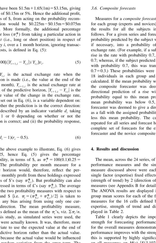
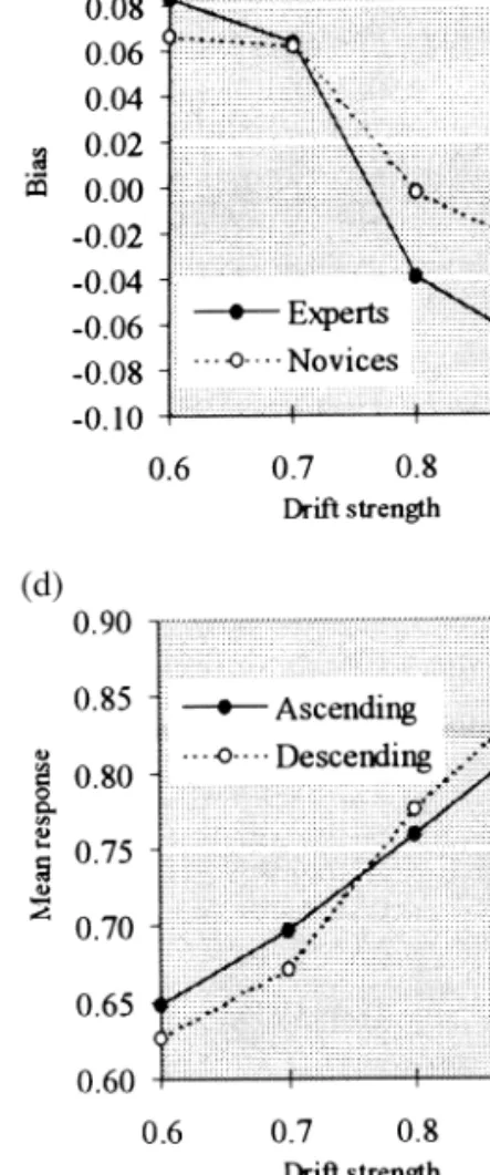
hF(3,102) 5 884.16, P , 0.001j. mild trend condition (drift strength of 0.6), while The direction of trend appears to influence the displaying more underconfidence than novices for relative accuracy (as indexed by URMPS hF(1,102) 5 strong and very strong trend conditions (drift 5.72, P , 0.05j), as well as M(p) hF(1,102) 5 37.79, strengths of 0.8 and 0.9). Fig. 1b may also be

P , 0.001j), with no significant effects on the mean interpreted as revealing evidence of the hard–easy weighted outcome index, mean probability response, effect, with overconfidence on the more difficult and bias (under / overconfidence). trends (i.e., trends that are harder to discern, with Regarding expertise, Table 1 shows a significant drift strengths of 0.6 and 0.7) and underconfidence inverse expertise effect on overall URMPShF(1,34) 5 on the less difficult trends (i.e., strong trends that are 7.17, P , 0.01j and on M(p) hF(1,34) 5 21.63, P , easier to detect, with drift strengths of 0.8 and 0.9). 0.001j, indicating better relative accuracy and higher Experts’ probability profiles are also largely re-profitability for novices’ directional probability fore- sponsible for the profitability differences shown in casts as compared to those of experts. A significant Fig. 1c. It can be seen that, while experts and main effect is also found for M(r)hF(1,34) 5 14.99, novices attain similar scores in the case of the

P , 0.001j, affirming the higher probabilities as- weakest trend, novices improve their profitability signed by the novice group. more than the experts as the trend gets stronger.

The main effects discussed above have to be Taken together, the results may be viewed as interpreted with caution, however, since Table 1 suggesting that the inferior overall performance of displays significant interactions for trend strength by the experts could be due to their underestimation of direction as well as trend strength by expertise. In strong trends (high magnitude drift). Perhaps, in particular, trend strength by expertise interactions are retrospect, this is not too surprising since these found for three of the performance measures: for individuals are likely to have been ‘nourished’ with

M(r)hF(3,102) 5 5.72, P , 0.01j, for B hF(3,102) 5 the Efficient Market Hypothesis (EMH) in the course 3.05, P , 0.05j, and for M(p) hF(3,102) 5 3.52, P , of their academic upbringing making them sceptical 0.05j. These interactions are illustrated in Fig. 1a, b that the stronger trends would continue into the and c, respectively, and in Table 2. Fig. 1a clearly future. Although the experts are clearly able to indicates that, although experts exhibited slightly recognise a trend, as illustrated in Tables 1 and 2, more confidence (as revealed by higher probability these individuals would always have in mind that assessments) than the novices on the weakest trend, trends can change in currency series and this together they were less able to accept the stronger trends, with an academic leaning towards random walk assigning lower probabilities than novices for drift theory may have resulted, in some instances, in an strengths of 0.7, 0.8 and 0.9. As a result of these explicit search for randomness in the face of con-mean probability profiles of experts and novices, we tradictory evidence. That is, these subjects may have can observe from Fig. 1b that experts appear to be had a tendency to view trends, to a larger extent than

(9)

Table 2

Mean performance scores for trend strength, direction and expertise Trend strength Performance measures

and direction M(c)(↑) URMPS(↓) M(r) B(0) M(p)(↑) Experts 0.6 — Pos. 0.570 1.261 0.662 0.091 0.003 0.6 — Neg. 0.556 1.267 0.630 0.075 0.002 0.6 — All (0.563) (1.264) (0.646) (0.083) (0.003) 0.7 — Pos. 0.619 0.835 0.666 0.047 0.006 0.7 — Neg. 0.596 0.796 0.676 0.080 0.006 0.7 — All (0.607) (0.816) (0.671) (0.064) (0.006) 0.8 — Pos. 0.767 0.506 0.730 20.36 0.017 0.8 — Neg. 0.800 0.361 0.759 20.41 0.023 0.8 — All (0.783) (0.433) (0.744) (20.039) (0.020) 0.9 — Pos. 0.885 0.361 0.813 20.072 0.036 0.9 — Neg. 0.900 0.281 0.828 20.072 0.046 0.9 — All (0.893) (0.361) (0.821) (20.072) (0.041) All h0.712j h0.708j h0.720j h0.009j h0.017j Novices 0.6 — Pos. 0.559 1.230 0.636 0.077 0.002 0.6 — Neg. 0.567 1.056 0.624 0.057 0.002 0.6 — All (0.563) (1.142) (0.630) (0.067) (0.002) 0.7 — Pos. 0.626 0.834 0.716 0.090 0.009 0.7 — Neg. 0.633 0.588 0.668 0.034 0.008 0.7 — All (0.630) (0.711) (0.692) (0.062) (0.009) 0.8 — Pos. 0.789 0.322 0.790 0.001 0.023 0.8 — Neg. 0.800 0.323 0.796 20.004 0.026 0.8 — All (0.794) (0.323) (0.793) (20.002) (0.025) 0.9 — Pos. 0.885 0.276 0.840 20.045 0.040 0.9 — Neg. 0.885 0.221 0.875 20.010 0.051 0.9 — All (0.885) (0.248) (0.858) (20.028) (0.046) All h0.718j h0.606j h0.743j h0.025j h0.020j

Experts and novices

0.6 — Pos. 0.565 1.245 0.649 0.084 0.003 0.6 — Neg. 0.561 1.161 0.627 0.066 0.002 0.6 — All (0.563) (1.203) (0.638) (0.075) (0.002) 0.7 — Pos. 0.622 0.834 0.691 0.069 0.007 0.7 — Neg. 0.615 0.692 0.672 0.057 0.007 0.7 — All (0.619) (0.743) (0.682) (0.063) (0.007) 0.8 — Pos. 0.778 0.414 0.760 20.018 0.020 0.8 — Neg. 0.800 0.342 0.777 20.023 0.025 0.8 — All (0.789) (0.378) (0.769) (20.020) (0.022) 0.9 — Pos. 0.885 0.318 0.826 20.058 0.038 0.9 — Neg. 0.893 0.251 0.852 20.041 0.048 0.9 — All (0.889) (0.285) (0.839) (20.050) (0.043) All h0.715j h0.657j h0.732j h0.017j h0.019j

Note:↑high values are best;↓low values are best; 0 zero is the best value.

novices, as being influenced by stochastic factors distant past, whereas the novices may have put more rather than deterministic factors (Wilkie-Thomson et emphasis on the overall trend.

al., 1997). The experts may also have been in- Table 1 also reveals significant trend strength by fluenced by the more recent changes in the series trend direction interactions on the M(r) measure (Tagaki, 1991) in comparison to changes in the more hF(3,102) 5 4.32, P , 0.01j, and on M(p)

(10)

(11)

hF(3,102) 5 16.58, P , 0.001j. These interactions for the individual cases on the stronger trends. are illustrated in Fig. 1d and e, respectively, and in Combining individual judgements on the stronger Table 2. Fig. 1d shows a clear pattern for the trends, therefore, failed to improve the bias score. subjects’ confidence levels in relation to the direction Instances where human composite forecasts sur-and strength of trend. Participants are less confident passed statistical models are worth noting. In terms (as revealed by lower mean probability responses) of URMPS, on the weakest trend, the novice compo-about negative trends than compo-about positive trends site, overall, achieved considerably better scores than when trends are weak (i.e., 0.6 and 0.7 trends), but both models. On the same measure, the novice the reverse is true when trends are strong (i.e., 0.8 composite, overall, surpassed the AR(1) model on and 0.9 trends). In terms of profitability, Fig. 1e the 0.8 trend. In relation to B, the two composites shows that, although performance is essentially outperformed both models on the weakest trend, and similar with upward and downward sloping series on the novice composites surpassed both models on the the weak (i.e., more difficult) trends, profitability 0.8 trend.

scores improve more for negatively-trended series In relation to profitability, however, as the compo-for the strong (i.e., less difficult) trends, with the site forecasts will always give identical profitability largest difference occurring on the strongest (i.e., for each forecast series as the group mean, there is

least difficult) trend. no direct benefit in combining forecasts from a

These analyses were further complemented by profitability viewpoint. comparing the groups’ mean scores to those of the

uniform or random walk forecaster (RW), the

ran-dom walk with constant drift (RWCD) and auto- 5. Conclusions and directions for future regressive order one (AR(1)) models, and human research

composite forecasts. These comparisons are

illus-trated in Table 3. Comparing the relative perform- As stated by O’Connor et al. (1997), ‘‘there ance of judgemental forecasts with those of the appears to be very little known about how people hypothetical random walk, Table 3 shows that the behave with trended time series’’ (p. 166). The subjects performed better on M(c) over all trends and current study has provided an exploratory step in on URMPS on the three strongest trends (i.e., drift investigating this important issue. Currency forecast-strength of 0.7, 0.8 or 0.9). These results compare ing is chosen as an exemplar domain where judg-favourably to those of previous probabilistic studies mental forecasts prevail, where their accuracy is of in the stock price forecasting domain (e.g., Stael von utmost importance, and where differences in trend Holstein, 1972; Yates, McDaniel & Brown, 1991; strength are commonly confronted. Using directional

¨

Onkal & Muradoglu, 1994) whose subjects have probability forecasts, we found that the strength of tended to perform worse than a random walk. trend has an important influence on all aspects of However, the subjects in the present study were forecasting performance studied. In particular, pre-generally outperformed by the more sophisticated dictive performance has been shown to improve with models (i.e., RWCD and AR(1)) on the various increasing trend strength. This finding may be ex-measures over the four trends. plained in conjunction with the hard–easy effect, As for composite versus individual judgement, in such that increasing drift strengths may be viewed as terms of overall performance, Table 3 shows that making the forecasting task easier. Accordingly, there was generally a slight improvement in the overconfidence is observed with the more difficult composite cases for M(c) and a dramatic improve- trends (i.e., trends that are harder to detect, with drift ment for URMPS. These findings are similar to those strengths of 0.6 and 0.7), while underconfidence is reported in Thomson, Pollock, Henriksen and displayed on the comparatively easier trends (i.e., Macaulay (in press). strong trends that are relatively easier to discern, However, in terms of B, although there was with drift strengths of 0.8 and 0.9). In fact, the considerable improvement in the composite cases on probability profiles of both the experts and the the weakest trend, performance was generally better novices provide support for the Lichtenstein and

(12)

Table 3

Performance scores for expertise, trend strength and direction: performance benchmarks and composite forecasts

Performance measures M(c)(↑) URMPS(↓) M(r) B(0) M(p)(↑) Trend strength 5 0.6 Experts — Pos. 0.570 1.261 0.662 0.091 0.003 Experts — Neg. 0.556 1.267 0.630 0.075 0.002 Novices — Pos. 0.559 1.230 0.636 0.077 0.002 Novices — Neg. 0.567 1.056 0.624 0.057 0.002 Uniform 0.500 1.000 0.500 0.000 0.000 RWCD 0.600 0.494 0.574 20.026 0.002 AR(1) 0.600 0.488 0.560 20.040 0.002

Comp. Exp — Pos. 0.600 0.281 0.607 0.007 0.003

Comp.Exp. — Neg. 0.600 0.549 0.585 20.015 0.002

Comp. Nov. — Pos. 0.600 0.371 0.604 0.004 0.002

Comp. Nov. — Neg. 0.600 0.305 0.599 20.001 0.002

Trend strength 5 0.7 Experts — Pos. 0.619 0.835 0.666 0.047 0.006 Experts — Neg. 0.596 0.796 0.676 0.080 0.006 Novices — Pos. 0.526 0.834 0.716 0.090 0.009 Novices — Neg. 0.533 0.588 0.668 0.034 0.008 Uniform 0.500 1.000 0.500 0.000 0.000 RWCD 0.700 0.129 0.698 20.002 0.010 AR(1) 0.700 0.077 0.697 20.003 0.010

Comp. Exp. — Pos. 0.700 0.730 0.587 0.020 0.006

Comp. Exp. — Neg. 0.567 0.426 0.616 20.084 0.006

Comp. Nov. — Pos. 0.700 0.687 0.672 0.105 0.009

Comp. Nov. — Neg. 0.700 0.332 0.650 20.050 0.008

Comp. Exp. — Pos. 0.800 0.327 0.713 20.087 0.017

Comp. Exp. — Neg. 0.800 0.160 0.760 20.040 0.023

Comp. Nov. — Pos. 0.800 0.102 0.793 20.007 0.023

Comp. Nov. — Neg. 0.800 0.121 0.809 0.009 0.027

Comp. Exp. — Pos. 0.900 0.254 0.808 20.092 0.036

Comp. Exp — Neg. 0.900 0.192 0.824 20.076 0.046

Comp. Nov. — Pos. 0.900 0.200 0.827 20.073 0.040

Comp. Nov. — Neg. 0.900 0.068 0.874 0.026 0.051

Note:↑high values are best;↓low values are best; 0 zero is the best value.

Fischhoff’s (1977) and Suantak, Bolger and Ferrell In general, the subjects were more overconfident (1996) findings in that overconfidence is reduced as on the weaker (more difficult) trends than they were mean weighted outcome index is increased from underconfident on the stronger (easier) trends, and 50% to 75%, with underconfidence emerging when this resulted in a low level of overconfidence overall. this index exceeds the 75% level. This finding disagrees with Bolger and Harvey’s

(13)

(1995) supposition that directional probabilistic fore- theory, their academic base may have induced these experts to search for randomness to correct any casting tasks would produce underconfidence, rather

‘misperceptions’ of strong trends. This supports van than the overconfidence that is normally observed in

Hoek’s (1992) proposition that ‘‘ . . . analysts appear confidence interval tasks (e.g., Lawrence &

Mak-to expect some reversal in recent exchange rate ridakis, 1989; Lawrence & O’Connor, 1993;

O’Con-movements or a return to some long-run ‘normal’ nor & Lawrence, 1989, 1992). Bolger and Harvey

value’’ (p. 467). Frankel and Froot (1990) and hypothesised that this would be the case since

Tagaki (1991) also report similar findings. Hence, an subjects in the directional situation are likely to

intriguing extension of current work may entail anchor and adjust (Tversky & Kahneman, 1974)

investigating the experts’ reactions to detailed task from the centre of the probability scale (Poulton,

¨ and / or performance feedback (Benson & Onkal, 1989, 1994), and insufficient adjustment away from

1992; Bolger & Wright, 1993, 1994; Muradoglu & this anchor would lead to hypoprecision or

under-¨

Onkal, 1994; Wright, Rowe, Bolger and Gammack, confidence. Conversely, when fractile judgements are

¨ ¨

required, the subject’s best single estimate tends to 1994; Onkal & Muradoglu, 1994, 1995, 1996; Onk-be used as an anchor, and adjusting away from this al-Atay, 1998).

point is likely to produce hyperprecision (Pitz, Another interesting result is given by the influence 1974), resulting in the overconfidence that is usually of trend direction on relative accuracy and observed. Given that the participants in the present profitability measures. The inferior performance on study attained a low level of overconfidence with positive trends reported in the present study supports their directional forecasts, current findings appear to the findings of Bolger and Harvey (1995) and contradict Bolger and Harvey’s assumption while Timmers and Wagenaar (1977), while disagreeing supporting Seaver von Winterfeldt and Edwards’ with the Lawrence and Makridakis (1989) results on (1978) results that their subjects’ judgements were prediction intervals. Why is this the case? Basic task ‘‘not too flat; they were about right, though not quite differences provide one potential answer. Task diffi-flat enough’’ (p. 384). The discrepancy between culty may offer another viable explanation. In the these findings and those of Bolger and Harvey could present study, participants’ forecasts reflected a be attributed to contextual factors, such as the sensitivity to differing growth rates, with the greatest labelling of time series. For instance, unlike the increasing-trend disadvantage occurring on the ‘sales’ label employed in the Bolger and Harvey strongest trend. Focusing only on upward-sloping study, our experts and novices were predicting under trends, Eggleton (1982) noted that the underestima-the ‘currency’ label. It has been suggested that underestima-the tion bias seemed to increase more than propor-subjects’ expectations about the behaviour of the tionately as growth rates increase. When growth is series may be affected by the particular labels used exponential, this underestimation bias on increasing (Goodwin & Wright, 1994), which may in turn alter trends appears to be substantial (Wagenaar & the participants’ reactions to trend. Future work to Sagaria, 1975; Wagenaar & Timmers, 1979). How-systematically delineate the effects of contextual ever, predictions from exponentially-decaying series information on predictive accuracy in domains where have been found to be much closer to those pre-differing trend strengths predominate remains vital scribed by the mathematical relationships (Timmers for the users and the providers of such forecasts. & Wagenaar, 1977). Therefore, the strength and the Regarding the effects of expertise, this study has direction of the slope appear to be important deter-found the experts’ forecasts to yield relatively low minants of performance, as highlighted by the sig-accuracy and profitability scores in comparison to the nificant interactions of trend strength with trend novices. The novice group has also been found to direction in the current study. Further work detailing use higher probabilities on average than the expert these potential effects remains crucial for designing group. These results, complemented by significant forecast support systems to enhance predictive ac-expertise by trend-strength interactions, may be curacy under differing trend conditions for diverse viewed as reflecting the experts’ resistance to accept application domains.

(14)

present study include the observed advantage of Appendix B. Model details composite forecasts over individual forecasts and

contexts enabling composite human judgement to Each of the performance measures was analysed surpass the performance of the statistical models. It as a single factor (expertise) fixed effects design is also worth noting that combining individual using 4 (strength of trend) by 2 (direction of trend) judgements, on stronger trends, failed to reduce bias. repeated measures. Specifically, the model assumed Composite forecasts and persistence of bias represent was

future research venues of interest.

Y 5m 1 a 1 b 1 (ab ) 1 d 1 (ad )

The accuracy of exchange rate forecasts is critical ijkm j k jk m jm

for both the users and the producers of financial _{1 (bd )} _{1 (abd )} ₁_g _{1 (bg )}

km jkm i( j ) ki( j )

information. Accordingly, profiling the effects of

1 (dg ) 1´

factors like trend strength that effectively alter mi( j ) (ijkm) predictive performance promises an important

re-where Y is the mean measured score (i.e.,

aver-search area worth pursuing. ijkm

aged over the 24 series) of the ith subject, expertise level j, trend k, direction m; a is the ‘expertise’j

effect, j 5 1 for experts, j 5 2 for novices; b is the

Appendix A. Subjects’ instruction sheet k

‘trend’ effect, k 5 1, 2, 3, 4 for mild, medium, strong and very strong drift, respectively; d is the

‘direc-Instructions for making the forecasts m

tion’ effect, m 5 1, 2 for upward trends (positive For each series we would like you to indicate,

drift) and downward trends (negative drift), respec-with a tick, the direction of movement of the series

tively; (ab ) is the expertise*trend interaction; in month 61 (1 month ahead forecast) relative to jk

(ad ) is the expertise*direction interaction; ( bd )

month 60. jm km

is the trend*direction interaction; (abd ) is the

Then we would like you to indicate how confident jkm

expertise*trend*direction interaction; g is the

you are in your choice by writing down a percentage i( j )

‘subject’ effect (subjects nested within expertise), of 50% to 100%. A value of 50% would mean that

i 5 1,2,3, . . . ,18; ( bg ) is the trend*subject inter-you are equally likely to be right or wrong — that is, ki( j )

action; (dg ) is the direction*subject interaction; your answer is completely a guess. A value of, say mi( j )

m is a constant (overall mean); a ’s are constants

60%, would indicate a greater degree of confidence j

such thatoa 5 0; b ’s are constants such that ob 5

in your response. A value of 100% indicates com- j k k

0; d ’s are constants such thatod 5 0; (ab ) ’s are

plete certainty that the series will move either up or m m jk

constants such that oo(ab ) 5 0; (ad ) ’s are

con-down. You should not, however, use values of less jk jm

stants such that oo(ad ) 5 0; (bd ) ’s are

con-than 50% as this would indicate that you are less jm km

stants such that oo(bd ) 5 0; (abd ) ’s are

con-likely to be right than wrong, in which case the km jkm

stants such that ooo(abd ) 5 0; g ’s are

con-alternative direction should be indicated as more jkm i( j )

stants such thatoog 5 0; (bg ) ’s are constants

likely. i( j ) ki( j )

2 such that ooo(bg ) 5 0; and ´ |_{N(0,s ).}

Three examples of how a hypothetical participant ki( j ) (ijkm) might respond are indicated below:

References

In which direction do you expect Probability of the series to move? being correct

(%) _{Ang, S., & O’Connor, M. (1991). The effect of group interaction} processes on performance in time series extrapolation.

Interna-Series X (a) rise œ 90%_]

] _{tional Journal of Forecasting,}_{7, 141–149.}

(b) fall _]

¨

Benson, P. G., & Onkal, D. (1992). The effects of feedback and Series Y (a) rise _] 70%_] _{training on the performance of probability forecasters.}

Interna-(b) fall œ _{tional Journal of Forecasting,}_{8, 559–573.} ]

Bolger, F., & Harvey, N. (1993). Context-sensitive heuristics in

Series Z (a) rise œ 50%_]

] _{statistical reasoning. The Quarterly Journal of Experimental}

(b) fall _]

(15)

Bolger, F., & Harvey, N. (1995). Judging the probability that the O’Connor, M., & Lawrence, M. (1989). An examination of the next point in an observed time-series will be below, or above, a accuracy of judgmental confidence intervals in time series given value. Journal of Forecasting,14, 597–607. forecasting. Journal of Forecasting,8, 141–155.

Bolger, F., & Harvey, N. (1996). Graphs versus tables: effects of O’Connor, M., & Lawrence, M. (1992). Time series characteris-data presentation format on judgmental forecasting. Interna- tics and the widths of judgmental confidence intervals. Interna-tional Journal of Forecasting,12, 119–137. _{tional Journal of Forecasting,}_{7, 413–420.}

Bolger, F., & Wright, G. (1993). Coherence and calibration in _{O’Connor, M., Remus, W., & Griggs, K. (1993). Judgmental} expert probability judgment. Omega,21, 629–644. _{forecasting in times of change. International Journal of} Bolger, F., & Wright, G. (1994). Assessing the quality of expert _Forecasting,_{9, 163–172.}

judgment: issues and analysis. Decision Support Systems,11, _{O’Connor, M., Remus, W., & Griggs, K. (1997). Going up–going}

1–24. _{down: how good are people at forecasting trends and changes}

Boothe, P., & Glassman, D. (1987). Comparing exchange rate _{in trends? Journal of Forecasting,}_{16, 165–176.}

forecasting models, accuracy versus profitability. Journal of _{Officer, L. H. (1982). Purchasing power parity and exchange} Forecasting,3, 65–79. _{rates: theory, evidence and relevance, Contemporary Studies in} Crumby, R. E., & Obstfeld, M. (1984). International interest rate _{Economic and Financial Analysis, Vol. 35. London: JAI.}

linkages under flexible exchange rates: a review of recent _¨

Onkal, D., & Muradoglu, G. (1994). Evaluating probabilistic evidence. In Bilson, J. F. O., & Marston, R. C. (Eds.),

forecasts of stock prices in a developing stock market. Euro-Exchange Rate Theory and Practice. Chicago: Chicago Press.

pean Journal of Operational Research,74, 350–358. Eggleton, I. R. C. (1982). Intuitive time-series extrapolation. _¨

Onkal, D., & Muradoglu, G. (1995). Effects of feedback on Journal of Accounting Research,20, 68–102.

probabilistic forecasts of stock prices. International Journal of Frankel, J., & Froot, K. (1990). The rationality of the foreign

Forecasting,11, 307–319. exchange rate: chartists, fundamentalists, and trading in the _¨

Onkal, D., & Muradoglu, G. (1996). Effects of task format on foreign exchange market. AEA Papers and Proceedings, 80,

probabilistic forecasting of stock prices. International Journal 181–185.

of Forecasting,12, 9–24. Goodwin, P., & Wright, G. (1993). Improving judgmental time

¨

Onkal-Atay, D. (1998). Financial forecasting with judgment. In series forecasting: a review of the guidance provided by

Wright, G., & Goodwin, P. (Eds.), Forecasting with Judgment. research. International Journal of Forecasting,9, 147–161.

Chichester: Wiley, pp. 139–167. Goodwin, P., & Wright, G. (1994). Heuristics, biases and

im-¨

Onkal-Atay, D., Wilkie-Thomson, M. E., & Pollock, A. C. provement strategies in judgmental time series. Omega, 22,

Judgemental forecasting. In: Clements, M. P., & Hendry, D. 553–568.

(Eds.), Companion to Economic Forecasting, Blackwell, in Harvey, N. (1995). Why are judgments less consistent in less

press. predictable task situations? Organizational Behavior and

Pitz, G. F. (1974). Subjective probability distributions for im-Human Decision Processes,63, 247–263.

perfectly known quantities. In Gregg, L. W. (Ed.), Knowledge Harvey, N., & Bolger, F. (1996). Graphs versus tables: effects of

and Cognition. New York: Wiley. data presentation format on judgemental forecasting.

Interna-Pollock, A. C. (1989). The time series characteristics of quarterly tional Journal of Forecasting,12, 119–137.

real and nominal lira / pound sterling exchange rate movements, Lawrence, M., & Makridakis, S. (1989). Factors affecting

1973–1988. Rivista di Matematica per le Scienze Economiche judgemental forecasts and confidence intervals. Organizational

e Sociali,12, 167–193. Behavior and Human Decision Processes,42, 172–187.

¨

Pollock, A. C., Macaulay, A., Onkal-Atay, D., & Wilkie-Thom-Lawrence, M., & O’Connor, M. (1992). Exploring judgemental

son, M. E. (1999). Evaluating predictive performance of forecasting. International Journal of Forecasting,8, 15–26.

judgmental extrapolations from simulated currency series. Lawrence, M., & O’Connor, M. (1993). Scale, variability and the

European Journal of Operational Research,114, 281–293. calibration of judgmental prediction intervals. Organizational

Pollock, A. C., & Wilkie, M. E. (1992). Currency forecasting: Behavior and Human Decision Processes,56, 441–458.

human judgment or models. VBA-Journaal,3, 21–29. Lichtenstein, S., & Fischhoff, B. (1977). Do those who know

Pollock, A. C., & Wilkie, M. E. (1993). Directional judgemental more also know more about how much they know.

Organiza-financial forecasting: trends and random walks. In Flavell, R. tional Behavior and Human Performance,20, 159–183.

(Ed.), Modelling Reality and Personal Modelling. Heidelberg: Lim, J. S., & O’Connor, M. (1995). Judgemental adjustment of

Physica, pp. 253–271. initial forecasts: its effectiveness and biases. Journal of

Be-Pollock, A. C., & Wilkie, M. E. (1996). The quality of bank havioral Decision Making,8, 149–168.

¨ forecasts: the dollar-pound exchange rate, 1990–1993. Euro-Muradoglu, G., & Onkal, D. (1994). An exploratory analysis of

pean Journal of Operational Research,91, 306–314. the portfolio managers’ probabilistic forecasts of stock prices.

Poulton, E. C. (1989). Bias in Quantifying Judgements. Hove and Journal of Forecasting,13, 565–578.

London: Lawrence Erlbaum Associates. Murphy, A. H., & Winkler, R. L. (1984). Probability forecasting

Poulton, E. C. (1994). Behavoural Decision Theory: A New in meteorology. Journal of the American Statistical

Associa-Approach. Cambridge: Cambridge University Press. tion,79, 489–500.

Nelson, C. R., & Plosser, C. I. (1982). Trends and random walks Remus, W., O’Connor, M., & Griggs, K. (1995). Does reliable in macroeconomic time series: some evidence and implications. information improve the accuracy of judgmental forecasts? Journal of Monetary Economics,8, 139–162. International Journal of Forecasting,11, 285–293.

(16)

Remus, W., O’Connor, M., & Griggs, K. (1996). Does feedback Wilkie, M. E., & Pollock, A. C. (1996). An application of improve the accuracy of recurrent judgmental forecasts? Or- probability judgement accuracy measures to currency forecast-ganizational Behavior and Human Decision Processes, 66, ing. International Journal of Forecasting,12, 25–40.

22–30. Wright, G., Rowe, G., Bolger, F., & Gammack, J. (1994).

Sanders, N. R. (1992). Accuracy of judgmental forecasts: a Coherence, calibration, and expertise in judgmental probability comparison. Omega,20, 353–364. forecasting. Organizational Behavior and Human Decision Seaver, D. A., von Winterfeldt, D., & Edwards, W. (1978). Processes,57, 1–25.

Eliciting subjective probability distributions on continuous Yates, J. F. (1982). External correspondence: decompositions of variables. Organisational Behavior and Human Performance, the mean probability score. Organisational Behavior and

21, 379–391. Human Performance,30, 132–156.

Stael von Holstein, C. A. S. (1972). Probability forecasting: an Yates, J. F., McDaniel, L. S., & Brown, E. S. (1991). Probabilistic experiment related to the stock market. Organisational Be- forecasts of stock prices and earnings: the hazards of nascent havior and Human Decision Performance,8, 139–158. expertise. Organisational Behavior and Human Performance, Suantak, L., Bolger, F., & Ferrell, W. R. (1996). The hard–easy 49, 60–79.

effect in subjective probability calibration. Organizational Behavior and Human Decision Processes,67, 201–221.

Biographies: Mary E. THOMSON is a Reader in the Division of Tagaki, S. (1991). Exchange rate expectations: a survey of survey

Risk, Glasgow Caledonian Business School. She completed a studies. IMF Staff Papers,38, 156–183.

Ph.D. on judgement in currency forecasting and has published Timmers, H., & Wagenaar, W. A. (1977). Inverse statistics and

articles and papers in a variety of books and journals in this area. misperception of exponential growth. Perception and

Psy-Her research interests focus on the role of judgement in financial chophysics,21, 558–562.

forecasting and decision making. Thomson, M. E., Pollock, A. C., Henriksen, K. B., & Macaulay,

A. The influence of the forecast horizon on the currency

¨

Dilek ONKAL-ATAY is an Associate Professor of Decision predictions of experts, novices and statistical models. European

Sciences and Associate Dean of the Faculty of Business Adminis-Journal of Finance.

tration at Bilkent University, Turkey. She received a Ph.D. in Tvede, L. (1990). The Psychology of Finance. Norway:

Nor-Decision Sciences from the University of Minnesota, and is doing wegian University Press.

research on decision analysis and probability forecasting. She has Tversky, A., & Kahneman, D. (1974). Judgement under

uncertain-published in the European Journal of Operational Research, ty: heuristics and biases. Science, 1127–1131.

International Forum for Information and Documentation, Interna-van Hoek, T. H. (1992). Explaining mark / dollar and yen / dollar

tional Journal of Forecasting, Journal of Behavioral Decision exchange rates in the 1980s. Economics Letters,38, 467–472.

Making, and the Journal of Forecasting. Wagenaar, W. A., & Sagaria, S. D. (1975). Misconceptions of

exponential growth. Perception and Psychophysics, 18, 416–

422. _{Andrew C. POLLOCK is a Lecturer in the Department of}

Wagenaar, W. A., & Timmers, H. (1979). The pond and duckweed _{Mathematics, Glasgow Caledonian University. He completed a} problem: three experiments on the misperception of economic _{Ph.D. on exchange rates in 1988, and has subsequently published} growth. Acta Psychologica,43, 239–251. _{a variety of articles and papers in this area. His particular research} Webby, R., & O’Connor, M. (1996). Judgemental and statistical _{interest is the application of analytical techniques to the}

forecast-time series forecasting: a review of the literature. International _{ing of currency and, more generally, financial time series.} Journal of Forecasting,12, 91–118.

¨

Wilkie-Thomson, M. E., Onkal-Atay, D., & Pollock, A. C. (1997).

Alex MACAULAY is Senior Lecturer in Statistics at Glasgow Currency forecasting: an investigation of extrapolative

judg-Caledonian University. He has a B.Sc. in Mathematics and an ment. International Journal of Forecasting,13, 509–526.

M.Sc. in Statistics (Stochastic Processes). He has a particular Wilkie, M. E., & Pollock, A. C. (1994). Directional currency

research interest in the forecasting of financial price series and in forecasting: an investigation into probability judgement

accura-the evaluation of predictive performance. ´

cy. In Peccati, L., & Viren, M. (Eds.), Financial Modelling. Heidelberg: Physica, pp. 354–364.