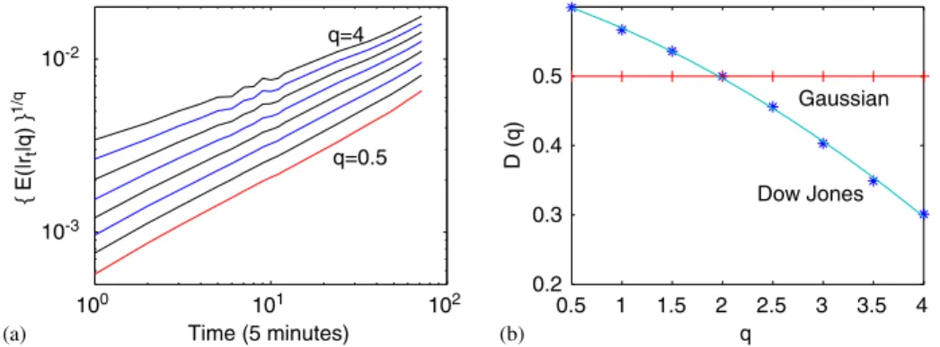
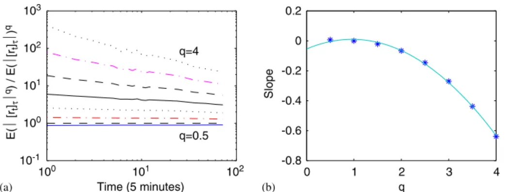
Intraday dynamics of stock market returns and volatility

Introduction and Aims: We prepared a center and physician based questionnaire to have an opinion of hemodialysis physicians about the quality indicators and the most

PLSVC: Persistent Left Superior Vena Cava; CRT: Cardiac Resynchronization Therapy; CS: Coronary Sinus; LV: Left Ventricular; NYHA: New York Heart Association; CT: Computed

The aim of the current study was to investigate the frequency of metabolic syndrome and C-reactive protein (CRP) levels, as a marker of systemic inflammation in stable COPD

Intramolecular charge transfer requires fluorophore and receptor to be linked in the electron system in which there are donor and acceptor groups. Sensors working based

Also, Mercan and Erenguc [8] developed a heuristic procedure for a similar problem, but with capacity constraints on the setup time.. Their objective was to minimize the

Bu proje çalışmasında, Emotiv EEG Neuroheadset cihazı kullanılarak kararlı durum görsel uyaranlar kullanılarak elde edilen EEG işaretlerinin doğru bir şekilde

In particular, Fujisawa and Kuh [ l l ] have shown that the Katzenelson's algorithm can be applied to (1) and it always converges to a solution as long as the equation has

Uniform alternate layer calix[8]acid/calix[4]amine LB thin films were prepared using the LB thin film deposition procedure, and the electrical properties for these LB thin films