MODEL DESCRIPTION OF FRICTION ON
PLANAR AND BUCKLED TWO DIMENSIONAL
MATERIALS
A THESIS SUBMITTED TO
THE GRADUATE SCHOOL OF ENGINEERING AND SCIENCE OF BILKENT UNIVERSITY
IN PARTIAL FULFILMENT OF THE REQUIREMENTS FOR THE DEGREE OF
MASTER OF SCIENCE IN
PHYSICS
By
Hasan Burkay Uzlu
January 2018
ii
FRICTION ANALYSIS ON TWO DIMENSIONAL MATERIALS VIA PRANDTL-TOMLINSON MODEL By Hasan Burkay Uzlu
January 2018
We certify that we have read this thesis and that in our opinion it is fully adequate, in scope and in quality, as a thesis for the degree of Master of Science.
___________________________________________ Oğuz Gülseren (Advisor)
___________________________________________ Mehmet Özgür Oktel
___________________________________________ Hande Toffoli
Approved for the Graduate School of Engineering and Science:
___________________________________________ Ezhan Karaşan
iii
ABSTRACT
MODEL DESCRIPTION OF FRICTION ON
PLANAR AND BUCKLED TWO DIMENSIONAL
MATERIALS
Hasan Burkay Uzlu M.S in Physics Advisor: Oğuz Gülseren
January 2018
The law of friction has been known since the 18th century but yet, the development on the tribology field was established in the last decades mainly by the invention of frictional force microscope (FFM), which enabled scientist to study friction on atomic levels. To describe the friction phenomena at nanoscale, molecular dynamics (MD) and density functional theory (DFT) models are commonly used, popular models and detailed information about friction can be obtained via those models. On the other hand, reduced-order simplified models such as Prandtl-Tomlinson (PT) model can also provide essential information about friction phenomena and understanding a phenomenon via a simplified model is always motivate.
In this thesis, Prandtl-Tomlinson model is generalized into three dimensions and the model is illustrated in both two and three dimensions on various quasi two dimensional crystal structures such as graphene, silicene, germanene and hexagonal boron nitride. By solving the equation of motion of the PT model numerically, friction curves and some parametric dependences of the friction such as anisotropy and friction dependence on external loading force is analyzed. We concluded that the PT model in three dimensions provides good results and can be used to analyze friction phenomena to save from computational cost in MD and DFT models.
iv
Keywords: graphene, friction, Prandtl-Tomlinson model, stick-slip motion,
v
ÖZET
DÜZLEMSEL VE BURULMALI İKİ BOYUTLU
MALZEMELERİN SÜRTÜNME ÖZELLİKLERİNİN
MODELLENMESİ
Hasan Burkay Uzlu Fizik, Yüksek Lisans Tez Danışmanı: Oğuz Gülseren
Ocak 2018
Sürtünme kuvveti kanunu 18nci yüzyıldan beri bilinmesine rağmen, sürtünme kuvveti hakkında araştırmalar 20nci yüzyılın sonlarına yakın yoğunlaşmış ve önemli gelişmeler görülmeye başlamıştır. Dokunmaya dayalı sürtünmeden ötürü malzemelere kalıcı hasar vermeden sürtünmenin araştırılması mümkün olmadığından, bu alanın gelişimi sürtünme kuvveti mikroskopunun icadıyla hız kazanmıştır. Sürtünme olayı hakkındaki teorik çalışmalar moleküler dinamik ve yoğun fonsiyonel teorisi (YFT) gibi metodlar ile yapılsa dahi, Prandtl-Tomlinson (PT) gibi indirgenmiş düzenli modeller de hızlı ve doğru sonuçlar verdiğinden ötürü önem taşıyan bir yaklaşım olmuştur.
Bu tezde, Prandtl-Tomlinson modeli üç boyutlu kullanılabilir hale getirilerek hem iki boyutta hem de üç boyutta çeşitli kristal yüzeyler üzerinde sürtünme kuvveti simülasyonları yapılmıştır. PT modelinin hareket denklemleri nümerik olarak çözülerek grafen, silisen, germanen ve boron nitrit gibi malzemeler üzerinde sürtünme kuvveti grafikleri elde edilip yöne ve harici yük kuvvetine bağlı sürtünme kuvveti hakkında analizler yapılmıştır. Simülasyonlarımızda elde edilen sonuçların deneysel veriler ile oldukça uyumlu olduğu görülmektedir ve PT modelinin sürtünme kuvvetini analiz etmek için diğer bilişsel zaman alıcı modellerin yanında basit, hızlı ve kullanışlı bir model olduğunu görüyoruz.
vi
Anahtar sözcükler: grafen, sürtünme kuvveti, Prandtl-Tomlinson modeli, kay-yapış
vii
Acknowledgement
I, first, would like to thank my supervisor Prof.Oğuz Gülseren for all his help and patient guidance. Without his guidance and support, this thesis could not be possible.
I would like to thank all physics department professors as well for being nice and patient all the time and showing much effort to teach us.
I also would like to thank my colleague Arash Mobaraki for helping me a lot during this thesis.
And I would like to thank Prof. Sinan Balcı, Dr. Osman Balcı, Dr. Nurberk Kakenov, Dr.Emre Ozan Polat for their support and guidance during my undergraduate and graduate years at Bilkent University
Finally, I would like to thank my family, especially to my sister Pelin Uzlu and brother-in-law Hakan Hacıahmetoğlu, and my dear friends Ali Demirtaş, Murat Özalp, Ozan Yakar and MD. Onur Karaoğlu for being supportive throughout my graduate years. I dedicate this work to my dear, lovely cat Louie.
viii
Contents
1 Introduction 1
1.1 Overview of friction and frictional force microscopy ... 1
2 Prandtl-Tomlinson model 5
2.1 Prandtl-Tomlinson model in 1D and 2D ... 5 2.2 Prandtl-Tomlinson model with temperature effect included ... 8 2.3 Numerical algorithm for Prandtl-Tomlinson model ... 9
3 2D Prandtl-Tomlinson model applications on graphene surface 12
4 3D modeling of Prandtl-Tomlinson method 23
4.1 3D simulation of PT model on graphene ... 24 4.2 Simulation with buckled structures and Friction relation with external loading force ... 30 4.3 Friction analysis on hexagonal boron nitride (hBN) ... 32
5 Conclusions 41
ix
List of Figures
Figure 1.1: Design of laser beam deflection method based friction force microscope. Here, cantilever torsion and deflection is measured by sensing the lateral and vertical deflections of the laser beam via photo-diodes. (Reproduced from G. Schitter et al. “High Performance feedback for fast scanning atomic force microscopes”, Review of scientific instruments, vol.72, no. 8, pp. 3320-3327, 2001) .. 3 Figure 2.1: Illustration of Prandtl-Tomlinson model. (Reproduced from Y.Dong,
A.Vadakkepatt and A. Martini, “Analytical Models for Atomic Friction”, Tribol Lett, vol.44, no 3, pp.367-386,2011) ... 5 Figure 2.2: Potential diagrams of PT model. (a) The tip is trapped in a local
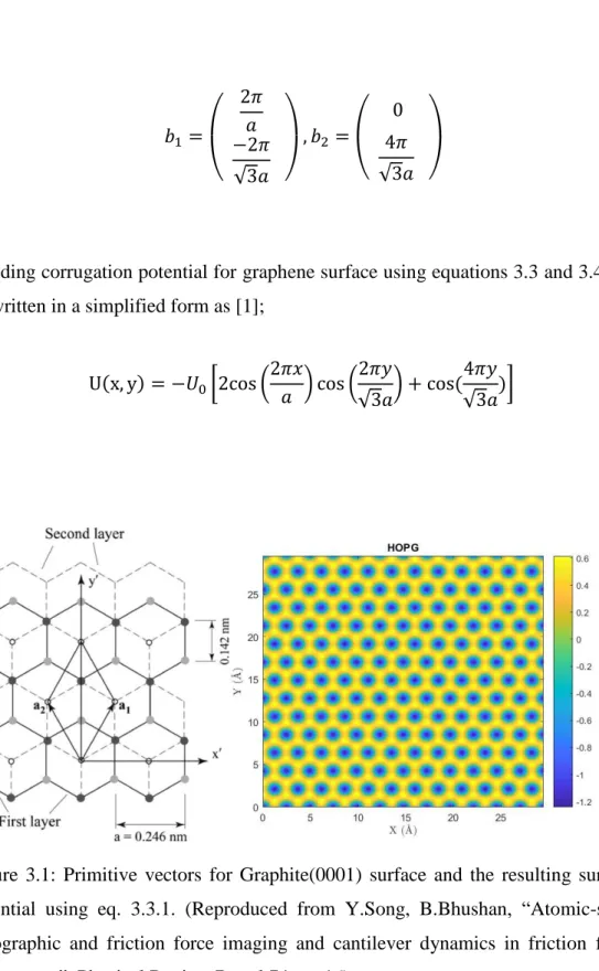
minimum and energy barrier prevents tip to jump to the next energy minimum. (b) Energy barrier is vanished due to the movement of the body support with velocity V, which results as a jump of the tip to the next local minimum. (Reproduced from H. Hölscher, A. Schirmeisen and U.Schwarz, “Principles of aromic friction: from sticking atoms to superlubric sliding”, Philosophical Transactions of the Royal Society A:Mathematical, Physical and Engineering Sciences, vol.366, no. 1869, pp. 1383-1404, 2008) ... 7 Figure 3.1: Primitive vectors for Graphite(0001) surface and the resulting surface
potential using eq. 3.3.1. (Reproduced from Y.Song, B.Bhushan, “Atomic-scale topographic and friction force imaging and cantilever dynamics in friction force microscopy”, Physical Review B ,vol.74, no 16) ... 13
x
Figure 3.2: Friction force simulation results for HOPG on zigzag (red) armchair (black) directions as a function of support displacement for temperature 0 Kelvin. ... 14 Figure 3.3: Friction force simulation results for HOPG on zigzag (red) armchair
(black) directions as a function of support displacement for temperature 300 Kelvin. ... 15 Figure 3.4: Trace of the tip during friction analysis with different scan-lines on
HOPG surface for temperatures 0 K and 300 K. ... 18 Figure 3.5: Trace of the tip during friction analysis with different scan-degrees
on HOPG surface for temperatures 0 Kelvin and 300 Kelvin. Sliding direction of the tip is 0°, 15°, 30°, 45°, 60° from the bottom to the top ... 20 Figure 3.6: Scan Degree dependent mean friction at T=0 (top) and T=300
(bottom) Kelvin. ... 21 Figure 3.7: Trace of the tip for HOPG surface at T=300K and at different scan
lines. Resolution is 1ms... 22 Figure 4.1: Friction force simulation results for HOPG on zigzag (red) armchair
(black) directions as a function of support displacement ... 25 Figure 4.2: Scan line dependence on HOPG surface for temperatures T=0 K
(top) and T=300 K (bottom). ... 26 Figure 4.3: Trace of the tip on HOPG surface for T= 0 K (top) and T=300
(bottom). Sliding direction of the tip is 0°, 15°, 30°, 45°, 60° from the bottom to the top ... 28 Figure 4.4: Scanning angle dependent mean friction at T=0 K (top) and T=300 K
xi
Figure 4.5: Trace of the tip for HOPG surface at T=300K and at different scan lines. Resolution is 0.5ms. Sliding direction of the tip is 0°, 15°, 30°, 45°, 60° from the bottom to the top ... 30 Figure 4.6: Structure of silicene and germanene. Reproduced from L.Yang et al.
“Revealing unusual chemical bonding in planar hyper-coordinate and quasi-planar two-dimensional crystals” PCCP, vol.17, pp.26043-26048,2015[37] ... 31 Figure 4.7: Frictional increase as a function of external loading force. For hBN,
is calculate by the formula and parameters are taken to be; eV, 11 eV eV, proportional with the values in section 4.3. ... 32 Figure 4.8: Schematic of hBN. Reproduced from N. Ooi et al., “Structural
properties of hexagonal boron nitride.” Modelling and Simulation in
Materials Science and Engineering, 2006. 14(3): p. 515-535. ... 33 Figure 4.9: Friction curve for hBN at T=0 Kelvin with scanning angle 0 ... 34 Figure 4.10: Trace of the tip on hBN surface at T=0 Kelvin with scanning angle
0 ... 35 Figure 4.11: Friction curve for hBN at T=0 Kelvin with scanning angle 30 ... 36 Figure 4.12: Trace of the tip on hBN surface at T=0 Kelvin with scanning angle
30 ... 36 Figure 4.13: Trace of the tip on hBN surface at T=0 Kelvin with different
scanning angles. Sliding direction of the tip is 0°, 15°, 30°, 45°, 60° from the bottom to the top ... 37 Figure 4.14: Trace of the tip on hBN surface at T=300 Kelvin with different
scanning angles. Sliding direction of the tip is 0°, 15°, 30°, 45°, 60° from the bottom to the top ... 38
xii
Figure 4.15: Scan Degree dependent mean friction at T=0 Kelvin for hBN... 39 Figure 4.16: Frictional increase as a function of external loading force for hBN .... 40
xiii
List of Tables
Table 2.1: 4th order time varying Runge-Kutta coefficients. ... 11 Table 2.2: Parameter values for simulation in 2D/3D with Prandtl-Tomlinson
1
Chapter 1
Introduction
1.1 Overview of friction and frictional force microscopy
Friction plays a significant role when two bodies are in contact and moving relative to each other. Because of that, tribology, called the study of friction, has quite of importance for all applications involving moving bodies in contact.[1-3]
Friction is defined to be the resistance against the motion of two in contact bodies relative to each other. This frictional force is defined as following;
where N is the normal force and is the friction coefficient that depends on moving bodies’ materials only. This is an empirical relation and called Antomon-Coulomb law of friction, which has no derivation method yet. This law of friction has been known since the 18th century but yet, the development on the field was established in the last decades mainly by the invention of frictional force microscope (FFM). Since experimenting friction without using any lubricant and causing any wear, bending or plastic deformation on body in both macroscopic and more importantly in microscopic level were quite difficult before FFM, attempts to study friction phenomena even for a simple –two in contact bodies moving relative to each other-
2
case were largely unsuccessful and the observation and analysis of pure, wearless friction are prevented for a long time.[4]
Major progress in the field has been accomplished by the establishment of the field of nanotribology. Basic idea of nanotribology can be summarized as first understanding the frictional behavior of single asperity contact and then explaining the frictional behavior on a macroscopic system with the help of statistics, which is briefly summing up whole the interactions of atomic contacts that forms the roughness of the contact interface of the macroscopic system. One vital experimental tool which makes experiments in atomic scale available is FFM.
The FFM is an atomic force microscopy (AFM) derivation and provides measurement of lateral forces between a surface and a sharp tip, where moving tip represents the single asperity contact over a sample surface. Working principle of AFM and FFM is as following:
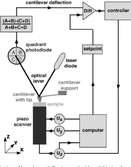
A tip (generally V shaped and provides the single asperity contact) is attached to a cantilever (leaf spring) and it detects the force acting between the tip itself and used sample surface. To map the surface topography, a feedback system controls the z-position (deflection) of the cantilever so that the force acting is always kept constant over the surface. Mapping all the xy-plane and detecting the force dependent z-position provides the surface topography[4]. This is briefly the working principle of AFM. In addition to that, AFMs modified to measure the torsion besides deflection is called frictional force microscope (FFM) and it is named as FFM since torsional force analysis provides the friction force between the tip and the surface. The most common detection method of deflection and torsion at FFMs is laser beam deflection method and Figure 1.1 provides the schematic for laser beam deflection method based FFM.
3
Figure 1.1: Design of laser beam deflection method based friction force microscope. Here, cantilever torsion and deflection is measured by sensing the lateral and vertical deflections of the laser beam via photo-diodes. (Reproduced from G. Schitter et al. “High Performance feedback for fast scanning atomic force microscopes”, Review of scientific instruments, vol.72, no. 8, pp. 3320-3327, 2001)
One significant advantage of frictional force microscopy is that experiments can be conducted in various environments like vacuum, ambient conditions or even in liquids [5, 6]. Also, wear and plastic deformation effects during the experiments can be prevented since the loading force of the system can be kept at low levels, which provide repeatable experiments and the analysis of pure, wearless friction. These
4
features and advantage of analysis of friction with single asperity contact, detecting the torsion caused by the tip and one individual atom on the surface at a time, provides FFM as a vital invention for tribologist.
The motion of FFM can also be modeled to understand friction phenomena computationally. Molecular dynamics (MD) calculations are a commonly used popular simulation to investigate friction at the atomic scale. It provides detailed information about each atom’s modal and energetic situation. Prandtl-Tomlinson (PT) and Frenkel-Kontorova (FK) models, on the other hand, are alternative, analytic reduced-order models that simplifies the simulation so that, one cannot obtain detailed atomistic information as MD simulation provides but still can describe the friction at the atomic scale under laboratory conditions[1-4]. In this thesis, PT model will be used generalized into three dimensions for some friction analysis (i.e. anisotropy) on planar and buckled systems. Anisotropy is the property of being directionally dependent, which implies different features in different directions[7]. Anisotropy in friction, on the other hand, is started to gain strong attention because of its importance to innovative new designs of frictional interfaces. Recent experiments have shown important variations in the atomic friction for different sliding directions. Some experimental works at this respect have analyzed the behavior of the frictional force in quasi-crystalline surfaces, and on molecular complexes [8-12]. Thus, theoretical studies of anisotropy in the friction force over a wide type of lattices are important sources of information to understand such effects. The goal of this letter is to determine the angular dependence of friction on hexagonal lattices like graphene and hBN.
5
Chapter 2
Prandtl-Tomlinson model
The simple and widely used reduced order model for atomic friction simulations is Prandtl-Tomlinson (PT) model, which consists of a harmonic spring and a mass attached to the end of that spring. In this chapter, equations of motions of PT model, numerical modeling method, temperature effect on frictional analysis and stick-slip motion of the harmonic spring in PT model will be discussed.
2.1 Prandtl-Tomlinson model in 1D and 2D
Schematic of the PT model is shown in Figure 2.1 below.
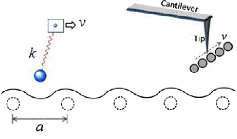
Figure 2.1: Illustration of Prandtl-Tomlinson model. (Reproduced from Y.Dong, A.Vadakkepatt and A. Martini, “Analytical Models for Atomic Friction”, Tribol Lett, vol.44, no 3, pp.367-386,2011)
6
Here, a point like tip (atomic size) is elastically coupled to a body M with harmonic spring with spring constant k. The support body M is moving with a constant velocity V in x direction and that provides tip to slide on periodically varying surface potential with lattice constant . The motion of this physical system can be formulated as following [13]:
where m is the mass of the tip, is the viscous friction (or damping constant) coefficient and U(x) is the potential of the surface. The terms on the right hand side represents the spring force, damping force that depends on the speed and force due to the tip and surface interaction. No surface dynamics (puckering around the tip, electron interactions etc.) are taken into consideration in this equation of motion. Solving this equation for x provides the friction force calculation via the relation .
̈ ̇
7
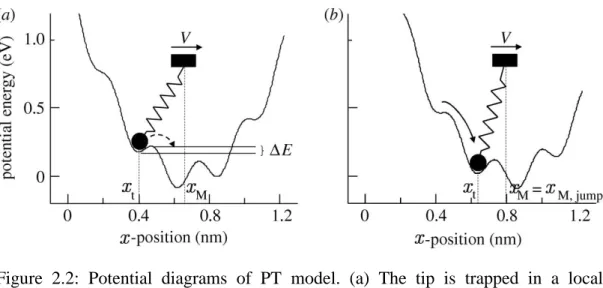
Figure 2.2: Potential diagrams of PT model. (a) The tip is trapped in a local minimum and energy barrier prevents tip to jump to the next energy minimum. (b) Energy barrier is vanished due to the movement of the body support with velocity V, which results as a jump of the tip to the next local minimum. (Reproduced from H. Hölscher, A. Schirmeisen and U.Schwarz, “Principles of aromic friction: from sticking atoms to superlubric sliding”, Philosophical Transactions of the Royal Society A:Mathematical, Physical and Engineering Sciences, vol.366, no. 1869, pp. 1383-1404, 2008)
The motion of the tip can be explained as following: Tip is assumed to be in equilibrium position at first in a local energy minimum and energy barrier prevents tip from moving to the next energy minimum. However, since the support body M moves in the x direction, energy barrier diminishes as time passes till the local minimum vanishes. At that point where the local minimum vanishes completely ( in Figure 2.2), tip jumps to the next local minimum and rests there till the energy barrier here that prevents tip jumping to the next minima vanishes completely due to the movement of the support body and so on[14, 15]. This stick-slip motion keeps repeating itself as the support body is scanned over the sample surface.[2, 3, 16, 17]
8
2.2 Prandtl-Tomlinson model with temperature effect included
When the value of energy barrier comes close to the value of (0.026 eV at room temperature), thermal effects cannot be neglected and for single asperity contact friction analysis, this energy barrier is generally on the order of 1 eV and thus, thermal effects plays a significant role on analysis of friction. As stated in the previous section, in the absence of thermal effects, tip slips only if energy barrier disappears, i.e. . In the presence of thermal effects, on the other hand, slip motion can occur sooner such that, when . So, the direct contribution of temperature to the system is a decrease of friction with the help of thermal energy to the tip to jump through potential energy barriers [18, 19]. Modifying our equation of motion (eq. 2.1) by adding temperature effect and putting the potential aroused from the spring and tip interaction into the corrugation potential results as the following equation of motion:[16, 18, 20]
where describes the surface potential plus the elastic potential due to the spring system and is a Gaussian random variable force field, describing the thermal activation force and satisfies the fluctuation-dissipation relation: . Equation of motion given above composed of deterministic and stochastic terms. The deterministic terms are; viscous drag resisting the movement of the tip and force due to the interaction between the tip and sample surface. Stochastic term is relates the strength of thermal force or fluctuating force to the damping constant of the friction or dissipation [11, 21-23].
Generalizing PT model for 2D surfaces is simple and obviously, we need to use 2D potential for defining the sample surface. Equations of motion are as following for 2D Prandtl-Tomlinson model:
̈ ̇
9
where , and is a random variable uniformly distributed between [ ]. Solving equations 2.2.2 and 2.2.3 by using the parameters [24] shown in Table 2.1, trajectory of the tip on the sample surface can be obtained and thus the lateral force (frictional force) on x and y directions can be calculated via relations and respectively.
2.3 Numerical algorithm for Prandtl-Tomlinson model
Equations above (eq. 2.2.2 and 2.2.3) cannot be solved analytically since they are not deterministic equations but, stochastic differential equations due to the thermal activation term. So, in order to simulate the physical system (PT model), 4th order Runge-Kutta algorithm is used. To apply this method, second order equations are reduced to first order differential equations as following[25]:
where and ̇ are parameters to reduce the order of initial equation of motions. Defining vectors and knowing the value for ( ) at time step , using the fourth order Runge-Kutta algorithm we can obtain the value for at time as;
̈ ̇ 2.2.2 ̈ ̇ 2.2.3 ( ̇ ̇ ) ( ) ( ) 2.3.1
10
where , and are Runge-Kutta slopes and coefficients shown in Table 2.1, t is the time step,
, j = 2 to n where n is 4 for 4th order algorithm and
values are random variables with Gaussian distribution with zero mean and variance value of 1. [ √ ( *] * ( ∑ ) √ ( *+ 2.3.2 2.3.3
11
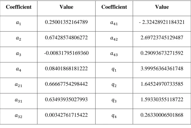
Table 2.1: 4th order time varying Runge-Kutta coefficients.
Coefficient Value Coefficient Value
0.25001352164789 - 2.32428921184321 0.67428574806272 2.69723745129487 -0.00831795169360 0.29093673271592 0.08401868181222 3.99956364361748 0.66667754298442 1.64524970733585 0.63493935027993 1.59330355118722 0.00342761715422 0.26330006501868
Table 2.2: Parameter values for simulation in 2D/3D with Prandtl-Tomlinson model. Variable Value m- Tip mass kg U-Potential amplitude 0.5/7 eV v- Scan velocity 400 Å/s k- Spring constant 25 N/m - Lattice constant 2.46 Å - Damping Coefficient √ ⁄ T- Temperature 0-300 Kelvin
12
Chapter 3
2D
Prandtl-Tomlinson
model
applications on graphene surface
In this section, two dimensional simulations of PT model for graphene analysis on friction phenomena, such as anisotropy, will be shown. First, corrugation potential term in equation 2.1 is calculated by the first term in Fourier expansion of the primary lattice vectors ( in Figure 3.1) as:
where ⃗ , ⃗ are reciprocal vectors and they can be calculated using the relation ⃗ . Using this information, simulations on graphene surface are shown
in this chapter.
For graphene surface, primitive and reciprocal vectors can be defined as following; ( ⃗ ) ⃗ 3.1 ( ) ( √ ) 3.2
13
Yielding corrugation potential for graphene surface using equations 3.3 and 3.4 can be written in a simplified form as [1];
Figure 3.1: Primitive vectors for Graphite(0001) surface and the resulting surface potential using eq. 3.3.1. (Reproduced from Y.Song, B.Bhushan, “Atomic-scale topographic and friction force imaging and cantilever dynamics in friction force microscopy”, Physical Review B ,vol.74, no 16)
( √ ) ( √ ) 3.3 [ ( * ( √ * √ ] 3.5
14
Tip is placed on the hollow site of the lattice and using the parameters shown in Table 2.2, following friction results are obtained on both zigzag and armchair directions.
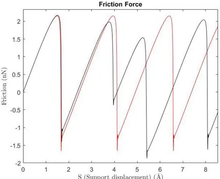
Figure 3.2: Friction force simulation results for HOPG on zigzag (red) armchair (black) directions as a function of support displacement for temperature 0 Kelvin.
15
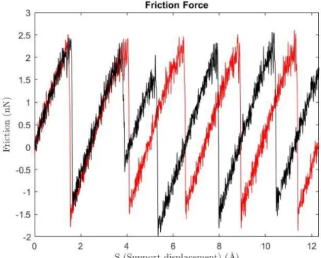
Figure 3.3: Friction force simulation results for HOPG on zigzag (red) armchair (black) directions as a function of support displacement for temperature 300 Kelvin.
Discontinuous, stick-slip motion of the tip can clearly be seen in Figure 3.2 and Figure 3.3. As expected, mean friction is decreased from 0.63 nN down to 0.5954 nN as the temperature is increased from 0 K to 300 K. Mean friction defined here is the mean of the curve from the first peak to the last peak in friction figures above. Stick-slip motion can be understood from the friction graph. This result suggests that our choices of parameters are a good fit to observe stick-slip motion. Stick-slip motion can be observed if the condition;
[
16
is satisfied and for the potential we used, that corresponds to the condition ⁄ . Otherwise, if ⁄ no discontinuous motion and no dissipation can be observed, tip will slide continuously along the surface sample without jumping from one potential minimum to another [26-29]. Value of corresponds to 4.18 with our choices of parameters. So, the results obtained are in consistent with the expectations. If we focus on the trace at finite temperature, we can see that the tip mostly prefers to stay at local minimums (hollow sites) of the potential as support moves. Also, we can observe more noisy motion of the tip and deflection from the path since stick slip motion can even occur when at finite temperatures.
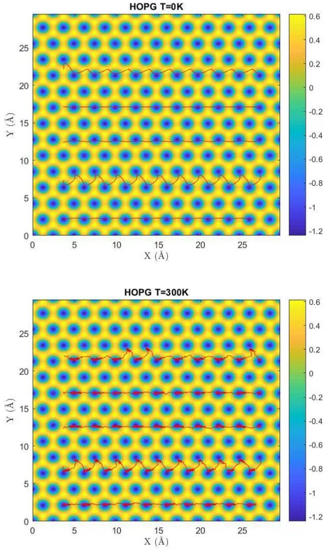
For deeper analysis of friction on graphene surface, first, scan line dependence of the friction is analyzed and Figure 3.4 shows that trace of the tip highly depends on the scanning line. Even if the support moves along a straight line, it can be seen from the figures that the tip can deviate and move through a zigzag pattern due to the 2D energy landscape. Trace depends so much on the starting point because of two basic reasons. Firstly, tip prefers to stay at the local minimums (hollow sites) and its motion basically consists of jumps into minimum points on the surface as the support body drags it. This motion analysis is shown in Figure 3.7. Secondly, the moving body in our model (representing the cantilever in the physical system) follows the scan line direction; it is not free to deviate as the tip. As a result, placing the support body on a hollow site and moving it onto x direction provides the trace of the tip as a straight line, since the tip jumps are through the minimums are on the x direction only (bottom lines in Figure 3.4). On the other hand, placing the support body on an atom causes the tip immediately jumping to a local minimum and as the surface is scanned, tip’s motion of jumping through local minimums creates a zigzag like trace (second line from the bottom in Figure 3.4.).
17
Deviation of the tip from a straight line is determined by the parameter . The bigger the value, the further the tip deviates from a straight line. In ideal case, force obtained via the simulation or experiment would reflect the gradient of potential along the scan line. However, this may not be the case every time due to the deviations of the tip depending on the value. Also, if we analyze the results obtained at finite temperature, at T=300 K, we can see that the tip can significantly deviate due to the thermal effects and that deflection shows how significant to consider thermal effects in PT model. Experimentally, AFM can be used to obtain surface profile by either keeping the force between the tip and surface constant and measuring the deflection or keeping the distance between the tip and surface constant and measuring the force. However, our results suggest that deviations from the scan line direction due the parameter choices and also the thermal effects may interrupt the surface analysis. PT model here offers another method to map surface topology of a surface since one can determine the hollow sites of the surface by analyzing the trace of the tip, since tip spends its most time in the hollow sites.
18
Figure 3.4: Trace of the tip during friction analysis with different scan-lines on HOPG surface for temperatures 0 K and 300 K.
19
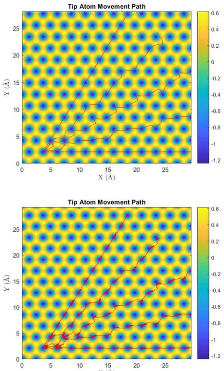
Secondly, we analyzed the direction dependence of the friction by scanning the support body with different angles in each simulation. Friction force is expected to be changed when we scan the surface with different angles since the tip will see different number of atoms in some directions with different periodicity (i.e. zigzag and armchair directions)[24, 30, 31]. Figure 3.5 and Figure 3.6 below show the position of the tip with different scan angles and the resulting mean friction. Hexagonal surface has 60° periodicity so any larger scanning degrees can be mapped back into degrees between 0° and 60° (i.e. 75° scanning is identical to 15° scanning)[31, 32]. As can be seen from the figures, different scanning angles cause different force patterns due to the 2D nature of potential energy. Experiments on anisotropy on graphene show up to 17% difference in the friction and the friction is observed to be higher on the armchair direction than the zigzag direction [24, 33-36]. In our simulation, up to 21% anisotropy on HOPG is observed and minimum frictional force is obtained on the armchair direction rather than on the zigzag direction. The difference between the experiment and our model here results from the tip-surface interaction in the experiment and that interaction increases as the tip moves along the sample surface due to the flexural deformations. Thus, friction is increasing as the tip moves along the surface. In our model, flexural deformations on the surface caused by the tip are not considered.
20
Figure 3.5: Trace of the tip during friction analysis with different scan-degrees on HOPG surface for temperatures 0 Kelvin and 300 Kelvin. Sliding direction of the tip is 0°, 15°, 30°, 45°, 60° from the bottom to the top
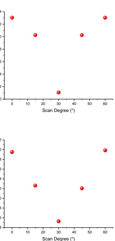
21 0 10 20 30 40 50 60 0,50 0,52 0,54 0,56 0,58 0,60 0,62 0,64 Me an F riction (n N) Scan Degree (°) 0 10 20 30 40 50 60 0,44 0,46 0,48 0,50 0,52 0,54 0,56 0,58 0,60 0,62 Me an F riction (n N) Scan Degree (°)
Figure 3.6: Scan Degree dependent mean friction at T=0 (top) and T=300 (bottom) Kelvin.
22
Friction can be more deeply understood if we time-resolve the trace of the tip and analyze its behavior. Figure 3.7 shows the time resolved plot of the trace of the tip for different scan lines. Data points on the plot is 1 ms apart from each other. As it can be seen, tip prefers to stay at a hollow site (local minimum) till the support body drags it out from that minimum and in that case, tip jumps into another minimum point on the surface. That result can be used to map accurately the surface potential of a sample by tracing the tip and finding the hollow sites of the sample with frictional force microscopy, since we know that the tip will spend its most time in local minimums.
Figure 3.7: Trace of the tip for HOPG surface at T=300K and at different scan lines. Resolution is 1ms.
23
Chapter 4
3D modeling of Prandtl-Tomlinson
method
In this chapter, 3D generalization of Prandtl-Tomlinson model will be provided by using Lennard Jones (LJ) potential instead of using sinusoidal potentials as in the previous chapters. One can define the interactions between the different atoms and define coordinate of each atom in a lattice precisely by LJ potential and thanks to that, besides graphene, one will be able to study structures consisting of different atoms like hexagonal boron nitride (hBN). Also, that feature of LJ potential enables us to examine buckled structures such as germanene and silicene by generalizing PT model into 3D. Equations of motions for the FFM tip in 3D can be written as following:
̈ ̇ 4.1 ̈ ̇ 4.2 ̈ ̇ 4.3
24
where is the loading force that is acting on the moving support body, which can be considered as the force acting on FFM cantilever in a physical system. As the potential term, following mathematical expression is used:
where represents the binding energy, represents the equilibrium distance[30]. During the following parts, using the above equations, 3D PT model is applied to the structures such as graphene, germanene, silicene and hBN. Anisotropy analysis and some analysis in z-direction beside the xy-plane friction analysis is provided. 20 atoms are set in y-direction and 30 atoms are set in x-direction during the all simulations and contributions of all of them to the corrugation potential are considered.
4.1 3D simulation of PT model on graphene
Tip is placed to a hollow site of the sample and using the parameters shown in Table 2.2 with no loading force (i.e. ) and, following results are obtained. Parameter is fitted to 7 eV to get similar friction results as in section three (compare Figure 3.2 and Figure 4.1).
∑
[( *
25
Figure 4.1: Friction force simulation results for HOPG on zigzag (red) armchair (black) directions as a function of support displacement
First, scan line dependence of the friction is tested as it is done in the previous section and the results are shown in Figure 4.2. Figures show that trace of the tip highly depends on the scanning line. As it is the case in 2D model, here as well, even if the support moves along a straight line, tip can deviate and move through different patterns due to the 3D energy landscape of the surface potential.
26
Figure 4.2: Scan line dependence on HOPG surface for temperatures T=0 K (top) and T=300 K (bottom).
27
Deviations from the scan line are observed due the larger parameter compared to the previous case. Figure 4.3 shows the path of the tip and time resolving it shows here again that the tip spends its most time in the hollow sites and its movement is basically consisting of jumping through a local minimum to another (Figure 4.5). Mean friction as a function of scanning angle is shown in Figure 4.4. Up to 21% change in the friction between the armchair and zigzag direction is observed in zero temperature case. However, anisotropy up to 33% is observed at finite temperature. Those results are in consistent with the results in section three even if there is a small difference. We believe, results in our 3D model are realistic and good results since LJ potential allows defining the coordinate of each atom precisely and thus provides a better determination of the surface potential.
28
Figure 4.3: Trace of the tip on HOPG surface for T= 0 K (top) and T=300 (bottom). Sliding direction of the tip is 0°, 15°, 30°, 45°, 60° from the bottom to the top
29 0 10 20 30 40 50 60 0,48 0,50 0,52 0,54 0,56 0,58 0,60 0,62 0,64 Me an F riction (n N) Scan Degree (°) 0 10 20 30 40 50 60 0,40 0,45 0,50 0,55 0,60 0,65 Me an F riction (n N) Scan Degree (°)
Figure 4.4: Scanning angle dependent mean friction at T=0 K (top) and T=300 K (bottom).
30
Figure 4.5: Trace of the tip for HOPG surface at T=300K and at different scan lines. Resolution is 0.5ms. Sliding direction of the tip is 0°, 15°, 30°, 45°, 60° from the bottom to the top
4.2 Simulation with buckled structures and Friction relation with external loading force
One good advantage of using 3D Prandtl-Tomlinson model is that one can study on buckled structures by describing the coordinate of each atom in three dimensional space and using the same parameters defined in part 4.1, friction analysis on germanene and silicene is provided in this part of the chapter. Schematic of the germanene and silicene structures are shown in Figure 4.6. Both materials have hexagonal structures like graphene but have different lattice constant and buckling parameters in z plane. For germanene, lattice constant is 4.43 Å and bucling 0.69 Å while the values for silicene are 3.845 Å and 0.44 Å respectively
31
Figure 4.6: Structure of silicene and germanene. Reproduced from L.Yang et al. “Revealing unusual chemical bonding in planar hyper-coordinate and quasi-planar two-dimensional crystals” PCCP, vol.17, pp.26043-26048,2015[37]
External loading force dependence of friction on graphene, silicene and germanene are shown below in Figure 4.7. As expected by the definition of friction (eq. 1.1), linear dependence of friction on loading force is obtained. Also, we can comment from the figure that the friction coefficient increases as the buckling of a system increases. Friction coefficients are calculated to be 0.018, 0.008, 0.144 and 0.215 for graphene, hBN, silicene and germanene respectively.
32 0 1 2 3 4 5 0,0 0,5 1,0 1,5 2,0 2,5 3,0 3,5 4,0 Me an F riction (n N) Loading Force (nN) Graphene Silicene hBN Germanene
Figure 4.7: Frictional increase as a function of external loading force. For hBN, is calculate by the formula √ and parameters are taken to be; eV, 11 eV eV, proportional with the values in section 4.3.
4.3 Friction analysis on hexagonal boron nitride (hBN)
One recently emerging material among other two dimensional materials is hBN, which have the structure similar to graphene [38]. Figure 4.8 shows the structure of a multilayer hBN. Boron and nitrogen atoms are bound via covalent bonds while the distinct layers are bound vie weak can der Waals forces as it is the case in multilayer graphene. During our simulation, we will be using one layer hBN.
33
Figure 4.8: Schematic of hBN. Reproduced from N. Ooi et al., “Structural
properties of hexagonal boron nitride.” Modelling and Simulation in Materials
Science and Engineering, 2006. 14(3): p. 515-535.
Following Lennard-Jones potential and parameters are used for the friction modeling.
Carbon tip is assumed to be used and in order to model the interaction between boron (B), nitrogen (N) and carbon (C) atoms. First, LJ parameters are adjusted accordingly[39]; √ and where i, j refer to B, N and C atoms. and meV, meV
∑
[( *
34
meV. Tip is located at z-position 3.4 at first and dragging it by moving the support body on hBN surface provided the following friction results; No stick slip motion, but the continuous periodic motion of friction is observed.
35
Figure 4.10: Trace of the tip on hBN surface at T=0 Kelvin with scanning angle 0
Figure 4.9 and Figure 4.11 shows the friction forces on armchair and zigzag directions. Periodicity in armchair direction is equal to the lattice constant and in zigzag direction, friction curve provides the information about the position of the tip successfully as well, whether the tip is passing above a hollow site or passing from one hollow site to another.
36
Figure 4.11: Friction curve for hBN at T=0 Kelvin with scanning angle 30
37
Here, as it is done in the previous sections, scanning angle dependence of friction in hBN is shown and it is observed that hBN shows significant directional dependence. Figures 4.13 and 4.14 show the trace of the tip on hBN surface with different scanning angles at zero and finite temperature.
Figure 4.13: Trace of the tip on hBN surface at T=0 Kelvin with different scanning angles. Sliding direction of the tip is 0°, 15°, 30°, 45°, 60° from the bottom to the top
38
Figure 4.14: Trace of the tip on hBN surface at T=300 Kelvin with different scanning angles. Sliding direction of the tip is 0°, 15°, 30°, 45°, 60° from the bottom to the top
Mean friction graph for the result at T=0 Kelvin is provided below in Figure 4.15. Up to 0.23% friction change is observed at zero temperature case. Simulation under the finite temperature case is dominated by the thermal noise as can be seen from the Figure 4.14.
39 0 10 20 30 40 50 60 0,02389 0,02390 0,02391 0,02392 0,02393 0,02394 0,02395 0,02396 Me an F riction (n N) Scan Degree (°)
Figure 4.15: Scan Degree dependent mean friction at T=0 Kelvin for hBN.
External loading force dependence of friction on hBN and other materials is shown below in Figure 4.16. A non-linear behavior, which is different than the behavior in Figure 4.7), but a general increase in the friction as the loading force increases is observed. Figure 4.8 is obtained under the friction analysis on stick-slip regime while the figure below is obtained in continuous, stick-slip free, regime. What we can conclude by comparing two graphs is that the dependence of friction on loading force shows a non-linear behavior in continuous regime while it shows a linear behavior in stick-slip regime.
40 0 1 2 3 4 0,0 0,2 0,4 0,6 0,8 1,0 Me an F riction (n N)
External Loading Force (nN)
Graphene hBN Silicene Germanene
41
Conclusions
Prandtl-Tomlinson model is generalized into three dimensions in this work by using LJ potential, which enables us to study buckled structures besides the planar structures and structures consisting of different atoms like hexagonal boron nitride. Two dimensional models are not sufficient to study such systems.
Significant similarity between the commonly accepted two dimensional PT model and developed 3D model is obtained. Comparing the tip paths at armchair and zigzag directions in two models shows a little difference but the anisotropy calculations provides similar results. At the armchair direction, tip’s deviation from his linear path is different in our 3D model and that difference causes change in the friction measurements and thus in the anisotropy analysis. We believe our developed 3D model is a good approach for friction analysis since LJ potential allows defining the coordinate of each atom precisely and thus provides a better determination of the surface potential than in 2D case since the surface potential in 2D model is determined by using the basic geometric aspects of the material used.
Also, friction analysis with loading force applied to the support body of FFM is simulated in the work. In stick slip regime (Figure 4.7), a linear dependence of friction, regardless of the material used, on loading force is observed while a non-linear dependence is observed in stick-slip free regime (Figure 4.16). Also, as expected, a general trend of increase in friction is observed as the buckling of the system increases.
42
For further analysis on friction, our 3D model can be applied on other quasi-two dimensional materials and even on multilayered structures. Also, considering flexural deformations on the sample surface caused by the tip will provide a good and more realistic comparison with the experimental results and thus, a better understanding of friction.
43
Bibliography
1. Dong, Y., A. Vadakkepatt, and A. Martini, Analytical Models for Atomic
Friction. Tribology Letters, 2011. 44(3): p. 367-386.
2. Holscher, H., D. Ebeling, and U.D. Schwarz, Friction at Atomic-Scale
Surface Steps: Experiment and Theory. Physical Review Letters, 2008.
101(24).
3. Holscher, H., A. Schirmeisen, and U.D. Schwarz, Principles of atomic
friction: from sticking atoms to superlubric sliding. Philosophical
Transactions of the Royal Society a-Mathematical Physical and Engineering Sciences, 2008. 366(1869): p. 1383-1404.
4. Binnig, G., C.F. Quate, and C. Gerber, Atomic Force Microscope. Physical Review Letters, 1986. 56(9): p. 930-933.
5. Song, Y.X. and B. Bhushan, Atomic-scale topographic and friction force
imaging and cantilever dynamics in friction force microscopy. Physical
Review B, 2006. 74(16).
6. Schitter, G., et al., High performance feedback for fast scanning atomic
force microscopes. Review of Scientific Instruments, 2001. 72(8): p.
3320-3327.
7. Park, J.Y., et al., Friction anisotropy: A unique and intrinsic property of
decagonal quasicrystals. Journal of Materials Research, 2008. 23(5): p.
1488-1493.
8. Choi, J.S., et al., Friction Anisotropy-Driven Domain Imaging on Exfoliated
Monolayer Graphene. Science, 2011. 333(6042): p. 607-610.
9. Dienwiebel, M., et al., Superlubricity of graphite. Physical Review Letters, 2004. 92(12).
10. Gnecco, E., Quasi-isotropy of static friction on hexagonal surface lattices. Epl, 2010. 91(6).
11. Muser, M.H., M. Urbakh, and M.O. Robbins, Statistical Mechanics of Static
and Low-Velocity Kinetic Friction. Advances in Chemical Physics, Vol 126,
44
12. Pina, C.M., R. Miranda, and E. Gnecco, Anisotropic surface coupling while
sliding on dolomite and calcite crystals. Physical Review B, 2012. 85(7).
13. Ermak, D.L. and H. Buckholz, Numerical-Integration of the Langevin
Equation - Monte-Carlo Simulation. Journal of Computational Physics,
1980. 35(2): p. 169-182.
14. Johnson, K.L. and J. Woodhouse, Stick-slip motion in the atomic force
microscope. Tribology Letters, 1998. 5(2-3): p. 155-160.
15. Medyanik, S.N., et al., Predictions and observations of multiple slip modes
in atomic-scale friction. Physical Review Letters, 2006. 97(13).
16. Gnecco, E., et al., Velocity dependence of atomic friction. Phys Rev Lett, 2000. 84(6): p. 1172-5.
17. Holscher, H., et al., Consequences of the stick-slip movement for the
scanning force microscopy imaging of graphite. Physical Review B, 1998.
57(4): p. 2477-2481.
18. Sang, Y., M. Dube, and M. Grant, Thermal effects on atomic friction. Physical Review Letters, 2001. 87(17).
19. Socoliuc, A., et al., Transition from stick-slip to continuous sliding in atomic
friction: Entering a new regime of ultralow friction. Physical Review
Letters, 2004. 92(13).
20. Jansen, L., et al., Temperature Dependence of Atomic-Scale Stick-Slip
Friction. Physical Review Letters, 2010. 104(25).
21. Dong, Y., et al., Thermal activation in atomic friction: revisiting the
theoretical analysis. Journal of Physics-Condensed Matter, 2012. 24(26).
22. Muser, M.H., Velocity dependence of kinetic friction in the
Prandtl-Tomlinson model. Physical Review B, 2011. 84(12).
23. Popov, V.L. and J.A.T. Gray, Prandtl-Tomlinson model: History and
applications in friction, plasticity, and nanotechnologies. Zamm-Zeitschrift
Fur Angewandte Mathematik Und Mechanik, 2012. 92(9): p. 683-708. 24. Almeida, C.M., et al., Giant and Tunable Anisotropy of Nanoscale Friction
in Graphene. Scientific Reports, 2016. 6.
25. Kasdin, N.J., Runge-Kutta Algorithm for the Numerical-Integration of
Stochastic Differential-Equations. Journal of Guidance Control and
Dynamics, 1995. 18(1): p. 114-120.
26. Fujisawa, S., et al., Fluctuation in 2-Dimensional Stick-Slip Phenomenon
45
Journal of Applied Physics Part 1-Regular Papers Short Notes & Review Papers, 1994. 33(6b): p. 3752-3755.
27. Fujisawa, S., et al., Atomic-Scale Friction Observed with a 2-Dimensional
Frictional-Force Microscope. Physical Review B, 1995. 51(12): p.
7849-7857.
28. Steiner, P., et al., Angular dependence of static and kinetic friction on alkali
halide surfaces. Physical Review B, 2010. 82(20).
29. Verhoeven, G.S., M. Dienwiebel, and J.W.M. Frenken, Model calculations
of superlubricity of graphite. Physical Review B, 2004. 70(16).
30. Dienwiebel, M., et al., Model experiments of superlubricity of graphite. Surface Science, 2005. 576(1-3): p. 197-211.
31. Park, J.Y., et al., High frictional anisotropy of periodic and aperiodic
directions on a quasicrystal surface. Science, 2005. 309(5739): p.
1354-1356.
32. Filippov, A.E., A. Vanossi, and M. Urbakh, Origin of Friction Anisotropy
on a Quasicrystal Surface (vol 104, 074302, 2010). Physical Review Letters,
2010. 104(14).
33. Ko, J.S. and A.J. Gellman, Friction anisotropy at Ni(100)/Ni(100)
interfaces. Langmuir, 2000. 16(22): p. 8343-8351.
34. Steiner, P., et al., Two-dimensional simulation of superlubricity on NaCl and
highly oriented pyrolytic graphite. Physical Review B, 2009. 79(4).
35. Weymouth, A.J., et al., Atomic Structure Affects the Directional
Dependence of Friction. Physical Review Letters, 2013. 111(12).
36. Zhang, Y., et al., Friction anisotropy dependence on lattice orientation of
graphene. Science China-Physics Mechanics & Astronomy, 2014. 57(4): p.
663-667.
37. Yang, L.M., et al., Revealing unusual chemical bonding in planar
hyper-coordinate Ni2Ge and quasi-planar Ni2Si two-dimensional crystals.
Physical Chemistry Chemical Physics, 2015. 17(39): p. 26043-26048.
38. Ooi, N., et al., Structural properties of hexagonal boron nitride. Modelling and Simulation in Materials Science and Engineering, 2006. 14(3): p. 515-535.
39. Neek-Amal, M. and F.M. Peeters, Graphene on boron-nitride: Moire