Principles of feedback control

170

Principles of

Feedback Control

170.2 Fundamentals of Feedback for Linear-Time-Invariant Systems

Open Loop Control • Feedback Control • Stabilization •

Tracking • Disturbance Attenuation • Sensitivity

In this chapter, fundamental properties of feedback control are discussed with engineering applications in mind. However, feedback appears in many other disciplines, such as agriculture, biology, medicine, pharmaceutics, economics, business management, political science, etc. A typical example of feedback control is steering of an automobile: we would like to keep the vehicle on the road (in the cruising lane). The road curvature determines the desired path to be followed. On the other hand, unpredictable gusting winds, bumps, or potholes on the road may move the vehicle off the cruising lane, unless corrective steering action is taken. As the driver (or autopilot) detects, using vision or other sensors, deviation from the desired path he/she can take the corrective steering action. Clearly, without the feedback from vision (or other sensory mechanism), the automobile cannot be kept on the road for a long time, even if we

know the desired path a priori. In this example, the position of the vehicle relative to the center of the

lane is the system output to be controlled, vision or another sensor provide a measured value of the

output to the controller (human driver or automatic steering mechanism). This information is processed

together with the desired path to be followed (i.e., reference input), and then steering angle (i.e., the

control input) is determined by the controller. The immeasurable variables such as wind, bumps, potholes,

as well as measurement errors due to imprecise sensing, represent the disturbances in this feedback system.

The main goal of feedback control is to reduce the effect of uncertainty (i.e., disturbances in the above example) on the output of the system. In fact, it is widely accepted by control engineers that the only reason to use feedback is to cope with uncertainty.

170.1 Feedback Control in Engineering

Generalizing the steering example given above, a feedback control system contains a process (a cause–effect

relation) whose operation depends on one or more variables (inputs) that cause changes in some other variables of interest (outputs). If an input can be manipulated, then it is said to be a control input;

otherwise it is considered as a disturbance, or noise. The controller compares the measured output (which

is obtained by a sensor) with the desired output (reference) and produces the control input for the process;

hence the feedback loop is closed (Figure 170.1). In typical engineering applications, the controller is a

computer, or a human interfacing with a computer. In this case, the control signal generated by a computer

Hitay Özbay

Bilkent University, Ankara Turkey on leave from The Ohio State University

170-2 The Engineering Handbook, Second Edition

needs to be converted to an input that the process takes. For example, in automatic steering applications discussed above, the computer generates a small electrical signal (in the form of a voltage or current) that needs to be converted to an angle of the steering column; typically, a DC motor does the job. Such

a device is called an actuator. The sensors and the actuators are interface devices between the physical

process and the controller. They are selected by the process engineer, depending on the physical appli-cation in mind, design specifiappli-cations, and economic considerations. The physical process together with

the actuators and sensors form the plant to be controlled.

In order to design a controller, a mathematical model of the plant (describing the dynamical behavior of the system) is derived. In the next section, I discuss systems represented by ordinary differential equations with constant coefficients, that is, finite-dimensional (lumped parameter) linear, time-invariant systems. Other types of mathematical models include infinite dimensional linear systems (e.g., systems with time delays, and spatially distributed systems described by partial differential equations), nonlinear dynamical systems, and fuzzy systems described by a set of logical rules. Control design techniques used depend on the type of dynamical equations representing the plant.

Typical goals in feedback controller design include: • Stability of the closed loop system

• Reduction of sensitivity to modeling uncertainty • Disturbance attenuation

• Tracking of a reference input

Clearly, in controller design the biggest concern is the first item in the above list. If the controller is not designed properly, a stable open-loop system (i.e., stable controller and stable plant connected in cascade with no feedback) may become unstable when the loop is closed with feedback. This is the main reason why feedback control is an important research area in engineering and applied mathematics.

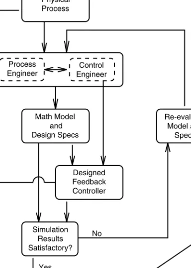
In practice, after a controller is designed for a physical system, it is tested under different operating conditions by performing numerical simulations and laboratory experiments. If the results are satisfac-tory, then the controller is deployed and the feedback loop is formed around the actual physical system. Otherwise, the mathematical model is refined, and/or some of the design specifications are relaxed in

order to satisfy all the design requirements. A summary of this process is shown in Figure 170.2.

170.2 Fundamentals of Feedback for Linear-Time-Invariant

Systems

In this section, to illustrate the benefits of feedback, we consider a simple control system, where the plant and the controller are single input–single output (SISO), linear, time-invariant systems whose transfer functions are rational functions. To further simplify the notation and discussion, we assume that the sensor is perfect (measured output is the same as the output of the process). Then, the feedback system shown in Figure 170.1 reduces to the system shown in Figure 170.3, where C(s) and P(s) are the transfer functions of the controller and the plant, respectively. (Plant transfer function is defined as P(s) = Y(s)/ U(s), where Y(s) and U(s) represent the Laplace transforms of the output y(t), and the input u(t),

respectively.) The tracking error, e, is defined as the difference between the reference input r and the

FIGURE 170.1 Feedback control system.

Controller Actuator Process

Sensor reference input control input output noise measured output Plant

Principles of Feedback Control 170-3

output y, that is, e(t) = r(t)- y(t). In Figure 170.3, the control input is u, and the disturbance is v. We want to make the tracking error “small” in the presence of disturbance and modeling errors in the plant.

Open Loop Control

First, consider the open loop control, where the Laplace transform of the output is given by

Y(s) = P(s)C(s)R(s) + P(s)V(s)

Clearly, when the plant is unstable, a small disturbance may result in an unbounded output. (A system is stable if its transfer function has no poles in {s : Re(s) ≥ 0}.) Even if we assume that v(t) = 0, to get a FIGURE 170.2 Controller design iterations.

FIGURE 170.3 Feedback system with controller C and plant P. Process Engineer Control Engineer Math Model and Design Specs Physical Process No Yes No Yes Re-evaluate Model and Specs Stop Iterations Simulation Results Satisfactory? Experimental Results Satisfactory? Designed Feedback Controller C(s) P(s) + + r (t) e(t) u(t) v(t) y (t) +_{_}

170-4 The Engineering Handbook, Second Edition

bounded output, the unstable poles of the plant must be cancelled by the zeros of the controller. As an example, let P(s) = 1/(s – 1), and consider a unit step reference input, R(s) = 1/s, with V(s) = 0. Then,

Assuming that C(s) does not have poles or zeros at s = 0 and s = 1, partial fraction expansion and

inverse Laplace transformation results in

where A = C(1), B = -C(0); and exponential decay, or growth, or oscillations in yc(t) depend on the

location of the poles of C(s). If the controller does not have a zero at s = 1, that is, if C(1) is not equal

to zero, y(t) is unbounded. So, in order to prevent an unbounded output, we must choose C(s) such that

C(1) = 0. It is clear from this example that a slightest uncertainty in the pole location of the plant will

lead to an unsuccessful controller design, and hence to an unbounded output. Thus, the open loop control is out of question when the plant is unstable; in this case, the uncertainty, either in the form of disturbance or in the form of modeling error, will lead to an unbounded output.

In light of the above discussion, now consider a stable plant, with no disturbance, v = 0. Then, in

order to make y(t)ª r(t), we tend to choose the open loop controller as C(s) = 1/P(s). There are two

problems with this choice: controller might turn out to be improper or unstable. As an example of the first case, let P(s) = 1/(s + 1), then C(s) = (s + 1), which is improper, that is, it contains a differentiator, and hence cannot be exactly implemented in a causal fashion. The second case occurs when the plant has a zero in the right half-plane, such as P(s) = (s - 1)/(s + 2). Taking the inverse of this plant leads to a controller whose pole is at s = 1, and again, the slightest uncertainty in the location of this right half-plane zero of the plant leads to an unbounded output.

Finally, for the open loop control, when r(t) = 0, and v(t) π 0, the system output is independent of the controller: Y(s) = P(s)V(s). We see that by using feedback we can attenuate the effect of this disturbance.

Feedback Control

As shown in Figure 170.3, feedback is formed by the equations

E(s) = R(s) - Y(s)

and

Y(s) = P(s)C(s)E(s) + P(s)V(s)

Therefore, the output is determined from the identity

(1 + P(s)C(s))Y(s) = P(s)C(s)R(s) + P(s)V(s)

Note that the right side of the above equality corresponds to the output of the open-loop control system discussed before. In order to determine Y(s) uniquely, the operator (1 + P(s)C(s)) must be causally

invertible; otherwise the feedback system is said to be ill-posed. For example, when P(s) = Kp and C(s)

= -1/Kp, the feedback system is ill-posed. Another example of an ill-posed systems is P(s) = 2s/(s + 1), C(s) = -1/2, in which case the inverse of (1 + P(s)C(s)) is (s + 1), an improper transfer function. In

general, the feedback system becomes ill-posed when

1 + P(•)C(•) = 0 Y s C c s s ( ) ( ) ( ) = -1 y t ( ) = Ae B y t , t + + c( ) for t>0

Principles of Feedback Control 170-5

From now on we assume that the feedback system is well-posed; and we define the sensitivity function,

S(s), as the inverse of (1 + P(s)C(s)). The word sensitivity will be defined shortly, and hence this notation

will be made clear.

In a well-posed feedback system the internal signals of interests are

E(s) = S(s)R(s) - S(s)P(s)V(s) U(s) = C(s)S(s)R(s) + S(s)V(s)

Stabilization

We say that a feedback system is bounded input/bounded output (BIBO) stable if every bounded input pair (r(t), v(t)) leads to bounded internal signals (e(t), u(t)). (A signal f(t) is said to be bounded if there exists a finite number Mf satisfying |f(t)| < Mf.)

It can be shown that the feedback system is BIBO stable if and only if transfer functions S(s), P(s)S(s), and C(s)S(s), are stable, that is, they have no poles in the closed right half-plane, {s : Re(s) ≥ 0}. It is important to note that stability of the plant and/or controller does not imply stability of the feedback system; conversely, stability of the feedback system does not imply stability of the plant nor the controller. In fact, one of the reasons to use feedback is to stabilize an unstable plant. For example, let P(s) = 1/(s - p), with p > 0, and C(s) = Kc, it is a simple exercise to show that closed loop system poles, that is, the

poles of S, PS, and CS, are the roots of

s - p + Kc = 0

Thus, with a simple gain Kc > p, we can stabilize the system using feedback. In order to have stability

robustness against a possible uncertainty in p, we might want to choose Kc much greater than the

maximum known value of p. Recall that with an open loop control scheme it is impossible to stabilize this system in the presence of uncertainty in p.

In general, feedback system stability can be determined by finding the closed loop system poles. Let P

= Np/Dp, and C = Nc/Dc, where Np, Dp, Nc, Dc are polynomials, and the pairs (Np, Dp) and (Nc, Dc) are

coprime. (A pair of polynomials (N, D) is said to be coprime if N(s) and D(s) do not have common roots.) Then, it is easy to see that all the poles of S, PS, and CS are precisely the roots of the characteristic equation

Dp(s)Dc(s) + Np(s)Nc(s) = 0

Once this equation is constructed, numerical root-finding tools can be used to calculate the closed-loop system poles. More discussion on stability analysis and controller design can be found in subsequent chapters of this handbook, where different design/analysis techniques are studied for more general classes of systems. In the remaining sections of this chapter on the fundamental properties of feedback, it is assumed that the feedback system is stable.

Tracking

One of the goals of feedback control is to make the output, y(t), track the reference input, r(t). Therefore, we would like to design the controller in such a way that the tracking error, e(t) = r(t) - y(t), is “small.” When v(t) ∫ 0, the Fourier transform of the error is E(jw) = S(jw)R(jw). Unless S ∫ 0, the error cannot be zero. So, the best we can do is make |S(jw)| “small” whenever |R(jw)| is not. For example, consider a unit step reference, R(s) = 1/s, and let P(s) = 1/(s - 1). Since R(0) = •, we need to have S(0) = 0, so that

E(0) π •. Since the plant does not have a pole at s = 0, in order to make S(0) = 0 the controller needs

170-6 The Engineering Handbook, Second Edition

to have a pole at s = 0. Accordingly, we choose a PI (proportional plus integral) controller whose transfer function is in the form C(s) = K(s + z)/s. The characteristic equation is

s2 _{+ (K - 1)s + Kz = 0}

For stability we need K > 1, and z > 0. Moreover, we can place the closed loop poles anywhere in the complex plane by properly selecting K and z. The tracking error is given by

If we place one of the closed loop poles at s = -1, and the other one at s = -r, then we have

This is achieved when K = r + 2, and z = r/(r + 2). Note that the right side of the above inequality can be made arbitrarily small by selecting large values of r; hence, the tracking error can be made small. On the other hand, it is a simple exercise to check that for the above design

u(t) = -1 + A exp(-rt) + B exp(-t)

where A = K(z - r)(r + 1)/(r(r - 1)), and B = 2K(1 - z)/(r - 1), and when r is large we have A ª K = r + 2. That leads to large values of |u(t)| in the transient response, possibly resulting in severe actuator damage or saturations. To summarize the discussion, in order to obtain good tracking performance we need use high gain controllers. However, the gain of the controller should not exceed a certain limit, determined by the actuator’s capacity to handle large inputs.

Disturbance Attenuation

In this section we assume that r(t) = 0, and v(t) π 0. Recall that in open loop control the output is Y(s)

= P(s)V(s), and hence the controller does not play a role in reducing the effect of disturbance on the

output. However, in feedback control, the output is Y(s) = S(s)P(s)V(s). Compared to the open loop response the output is scaled by a factor of |S(jw)| in the frequency domain. Therefore, as in the tracking discussion, whenever |V(jw)| is “large” we need to make |S(jw)| “small” by a proper choice of the controller

C(s). This way, the effect of the disturbance on the output can be reduced significantly. As an example,

consider a unit step disturbance V(s) = 1/s, for the unstable plant P(s) = 1/(s - 1), and let the feedback controller be the same PI controller defined above C(s) = K(s + z)/s. Then, the output due to disturbance

v is obtained as Y(s) = 1/(s2 _{+ (K - 1)s + Kz). Again, choosing K = r + 2 and z = r/(r + 2), we have}

Hence the output can be made as small as desired, provided that the actuator is not pushed to its limits.

Sensitivity

Consider a function F, which depends on a parameter a. Sensitivity of F with respect to variations of a is defined as E s s s K s Kz ( ) ( ) = -+ - + 1 1 2 E j j r r (w) / w = + £ 1 1 | ( )| ( )( )| Y j | j r j r w w w = + + £ 1 1 1 S F F F F F a a a a a = = ∂ ∂ D D / /

Principles of Feedback Control 170-7

where DF represents variations in F due to variations in a by an amount Da, at the nominal value of a. Therefore, the functions defined above need to be evaluated at the nominal value of a. Now let F to be the transfer function from r to y, denoted by T, and the parameter a be the plant transfer function, P. In the open loop case we have T = PC, and in the feedback control case T = 1 - S = PC/(1 + PC). Since

P is simply a “model” of the plant, it does not capture the “true” behavior of the actual plant. Accordingly,

assume that the “true” plant has a transfer function in the form P + DP, where DP represents the modeling uncertainty. By applying the above definition of the sensitivity, we find that sensitivity of T with respect to variations in P is 1 for the open loop control, and it is equal to 1/(1 + PC) for feedback control. Recall that 1/(1 + PC) = S, which we called the “sensitivity” function for the now obvious reason. Having unity sensitivity (open loop case) means that, any percentage variation of P will result in the same percentage variation in T. On the other hand, a properly designed controller can reduce the sensitivity (i.e., smaller than unity) in the frequency region of interest. Note that, by definition of the sensitivity, we have

and hence

Thus, we need to make the sensitivity |S(jw)| “small” whenever |DP(jw)C(jw)| is “large.” This property is also needed for stability robustness in the presence of plant uncertainty. For details, see subsequent chapters in this volume, and sources listed below.

References and Further Reading

Principles of feedback control and basic feedback system analysis and design techniques can be found in all undergraduate level textbooks on feedback control systems. Some of the newer texts include detailed discussions on the links between sensitivity and robustness, a topic that has been traditionally left for a second course on feedback control. A partial list of introductory textbooks on feedback control systems is given below.

P. R. Bélanger, Control Engineering: A Modern Approach, Saunders College Publishing, Fort Worth, TX, 1995.

R. C. Dorf and R. H. Bishop, Modern Control Systems, 9th ed., Prentice Hall, New York, 2001.

J. C. Doyle, B. A. Francis, and A. R. Tannenbaum, Feedback Control Theory, Macmillan, New York, 1992. G. F. Franklin, J. D. Powell, and A. Emami-Naeini, Feedback Control of Dynamic Systems, 4th ed., Prentice

Hall, New York, 2002.

G. C. Goodwin, S. F. Graebe, and M. E. Salgado, Control System Design, Prentice Hall, New York, 2001. B. C. Kuo, Automatic Control Systems, 7th ed., Prentice Hall, New York, 1995.

K. Ogata, Modern Control Engineering, 4th ed., Prentice Hall, New York, 2002. H. Özbay, Introduction to Feedback Control Theory, CRC Press, Boca Raton, FL, 2000. K. Morris, Introduction to Feedback Control, Harcourt/Academic Press, New York, 2001.

C. E. Rohrs, J. L. Melsa, and D. G. Schultz, Linear Control Systems, McGraw-Hill, New York, 1993. New developments in feedback control theory and their applications in many engineering disciplines are reported regularly in academic journals. The most prominent journals in this area, most of which are published monthly, are listed below.

IEEE Transactions on Automatic Control

IEEE Transactions on Control Systems Technology Automatica, journal of IFAC

DT D T S P P = DT=S P C SD

170-8 The Engineering Handbook, Second Edition

Control Engineering Practice, journal of IFAC SIAM Journal on Control and Optimization Systems & Control Letters

Mathematics of Control Signals and Systems International Journal of Control

International Journal of Robust and Nonlinear Control International Journal of Adaptive Control and Signal Processing European Journal of Control

AIAA Journal of Guidance Control and Dynamics

ASME Journal of Dynamic Systems Measurement and Control

The two largest professional societies active in the control systems area are:

Control Systems Society of IEEE (Institute of Electrical and Electronics Engineers): www.ieeecss.org

IFAC, International Federation of Automatic Control: www.ifac-control.org

Besides publishing some of the academic journals listed above, these societies regularly hold meetings devoted to the latest developments in the control systems area. Some of the major control conferences are:

Conference on Decision and Control, held once a year in December American Control Conference, held once a year in early summer

Conference on Control Applications, held once a year, typically in the summer European Control Conference, held once a year late summer

IFAC World Congress, held once every 3 years, typically in the summer.