A novel array signal processing technique for multipath channel parameter estimation

(1)

A NOVEL ARRAY SIGNAL PROCESSING

TECHNIQUE FOR MULTIPATH CHANNEL

PARAMETER ESTIMATION

a thesis

submitted to the department of electrical and

electronics engineering

and the institute of engineering and sciences

of bilkent university

in partial fulfillment of the requirements

for the degree of

master of science

By

Mehmet Burak G¨uldo˘gan

July 2006

(2)

I certify that I have read this thesis and that in my opinion it is fully adequate, in scope and in quality, as a thesis for the degree of Master of Science.

Prof. Dr. Orhan Arıkan(Supervisor)

Prof. Dr. Enis C¸ etin

Asst. Prof. Dr. ˙Ibrahim K¨orpeo˘glu

Approved for the Institute of Engineering and Sciences:

Prof. Dr. Mehmet Baray

(3)

ABSTRACT

A NOVEL ARRAY SIGNAL PROCESSING

TECHNIQUE FOR MULTIPATH CHANNEL

PARAMETER ESTIMATION

Mehmet Burak G¨uldo˘gan

M.S. in Electrical and Electronics Engineering

Supervisor: Prof. Dr. Orhan Arıkan

July 2006

Many important application areas such as mobile communication, radar, sonar and remote sensing make use of array signal processing techniques. In this thesis, a new array processing technique called Cross Ambiguity Function - Direction Finding (CAF-DF) is developed. CAF-DF technique estimates direction of ar-rival (DOA), time delay and Doppler shift corresponding to each impinging sig-nals onto a sensor array in an iterative manner. Starting point of each iteration is CAF computation at the output of each sensor element. Then, using incoherent integration of the computed CAFs, the strongest signal in the delay-Doppler do-main is detected and based on the observed phases of the obtained peak across all the sensors, the DOA of the strongest signal is estimated. Having found the DOA, CAF of the coherently integrated sensor outputs is computed to find accurate delay and Doppler estimates for the strongest signal. Then, for each sensor in the array, a copy of the strongest signal that should be observed at that sensor is constucted and eliminated from the sensor output to start the next it-eration. Iterations continue until there is no detectable peak on the incoherently integrated CAFs. The proposed technique is compared with a MUSIC based

(4)

technique on synthetic signals. Moreover, performance of the algorithm is tested on real high-latitude ionospheric data where the existing approaches have limited resolution capability of the signal paths. Based on a wide range of comparisons, it is found that the proposed CAF-DF technique is a strong candidate to define the new standard on challenging array processing applications.

Keywords: Array signal processing, direction of arrival (DOA), MUSIC, delay

(5)

¨

OZET

C

¸ OKLUYOL KANAL PARAMETRE KEST˙IR˙IM˙I ˙IC

¸ ˙IN YEN˙I

B˙IR D˙IZ˙I S˙INYAL ˙IS¸LEME TEKN˙I ˘

G˙I

Mehmet Burak G¨uldo˘gan

Elektrik ve Elektronik Mühendisli¯gi Bölümü Yüksek Lisans

Tez Y¨oneticisi: Prof. Dr. Orhan Arıkan

Temmuz 2006

Mobil haberle¸sme, radar, sonar ve uzaktan algılama gibi bir ¸cok ¨onemli

uygula-mada, dizi sinyal i¸sleme tekniklerinden faydalanılır. Bu tezde, C¸ arpraz Belirsizlik

Fonksiyonu - Y¨on Bulma (C¸ BF-YB) adında yeni bir dizi i¸sleme tekni˘gi

geli¸stirilmi¸stir. C¸ BF-YB tekni˘gi, bir algılayıcı dizisine gelen sinyallerden

her-birinin geli¸s yönünü (GY), zaman gecikmesini ve Doppler kaymasını yinelemeli

bir ¸sekilde kestirir. Herbir algılayıcı ¸cıktısındaki C¸ BF hesaplaması, yinelemelerin

ba¸slangı¸c noktasını olu¸sturur. Daha sonra, C¸ BF’lerin faz uyumsuz bir ¸sekilde

entegrasyonunu kullanarak, gecikme-Doppler alanındaki en gü¸clü sinyal tespit edilir ve tüm algılayıcılarda elde edilen tepe noktalarında gözlemlenen fazlar esas alınarak en gü¸clü sinyalin GY’si kestirilir. GY’yi bulduktan sonra, en gü¸clü sinyalin gecikme ve Doppler kaymasını kestirmek i¸cin, uyumlu entegre edilmi¸s dizi

¸cıktısının C¸ BF’si hesaplanır. Takiben, dizideki herbir algılayıcı i¸cin, aygılayıcıda

gözlemlenmesi gereken en gü¸clü sinyalin bir kopyası olu¸sturulur ve bir sonraki yinelemeyi ba¸slatmak i¸cin algılayıcı ¸cıktısından ¸cıkarılır. Faz uyumsuz olarak

entegre edilmi¸s C¸ BF’ler ¨uzerinde algılanabilecek tepe noktası kalmayıncaya

kadar yinelemeler devam eder. Sentetik olarak olu¸sturulmu¸s sinyaller

(6)

Ek olarak, algoritmanın peformansı, literat¨urdeki yakla¸sımların sinyal yollarını ayırmada sınırlı kabiliyetlere sahip oldu˘gu ger¸cek y¨uksek-enlem iyonosfer verileri

üzerinde test edilmi¸stir. Geni¸s bir yelpazede yapılan kıyaslamalara göre, Ç

BF-YB tekni˘gi karma¸sık dizi i¸sleme uygulamalarında standartları belirleyebilecek g¨u¸cl¨u bir adaydır.

Anahtar Kelimeler: Dizi sinyal i¸sleme, geli¸s y¨on¨u (GY), MUSIC, zaman gecikmesi

(7)

ACKNOWLEDGMENTS

I would like to express my thanks and gratitude to my supervisor Prof. Dr. Orhan Arıkan for his supervision, suggestions and invaluable encouragement throughout the development of this thesis. He is not only the best advisor that I have seen but also a role model as a researcher and a teacher to me. His intuition to see and solve a problem was amazing to me and it was a big pleasure to be advised by him.

I wish to thank Dr. Mike Warrington and his research group at the University of Leicester for the HF data, processing codes and for permission to use them in this thesis.

Special thanks to Prof. Dr. Feza Arıkan, Prof. Dr. Enis C¸ etin, and Asst. Prof.

Dr. ˙Ibrahim K¨orpeo˘glu, for their valuable comments and suggestions on the thesis.

I would like to thank Assoc. Prof. Dr. Ezhan Kara¸san, Assoc. Prof. Dr. Nail Akar and G¨uray G¨urel for their help and support in using the facilities at BINLAB.

I would also like to thank my colleagues in T ¨UB˙ITAK-UEKAE for their support

and encouragement during my graduate study.

Finally, I would like to say thanks to my mother,G¨und¨uz, and my sister,Berrak, for always believing in me and encouraging me to achieve my goals. My deepest gratitude goes to my wife, Seher, for her support and love which have been invaluable in helping me focus on my academic pursuits.

(8)

List of Figures

2.1 Direction of the signal and reference coordinate system. . . 7

2.2 Circular array and multipath enviroment. . . 8

2.3 IQ Detector. . . 12

2.4 Matched filter block diagram. . . 13

2.5 Ideal ambiguity function; ¯¯

χ

(τ, ν)¯¯2 = δ(τ, ν). . . 16

2.6 2D view of the ambiguity function for a single pulse of width τp. . 16

2.7 Ambiguity function distribution of an uniform pulse train. . . 18

2.8 Ambiguity function distribution of a Barker-13 sequence. . . 18

4.1 Electron production due to solar radiation. . . 33

4.2 Ionosphere layers. . . 34

4.3 Propagation modes. . . 37

4.4 Elevation angle fixed. . . 39

4.5 Path length fixed. . . 39

(12)

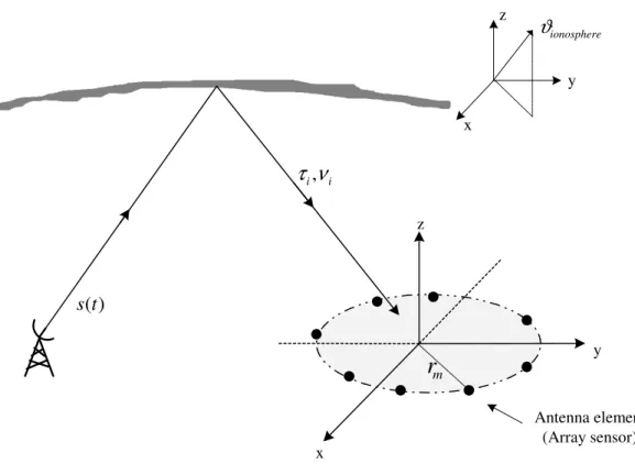
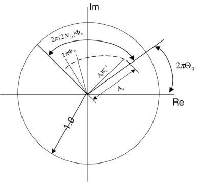
5.1 Signal transmitted to the ionosphere and reflected back to the sensor array. . . 44 5.2 z-domain circle . . . 49

5.3 Result of the CAF computation for the mth _{antenna output with}

transmitted signal when only one signal path exists. . . 51

5.4 Result of the CAF computation for the mth _{antenna output with}

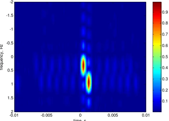
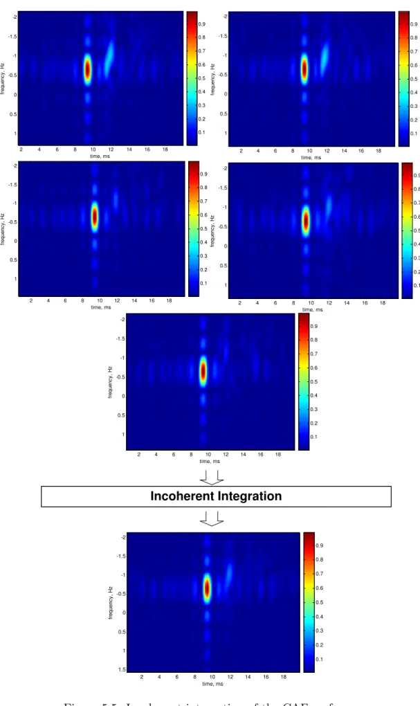
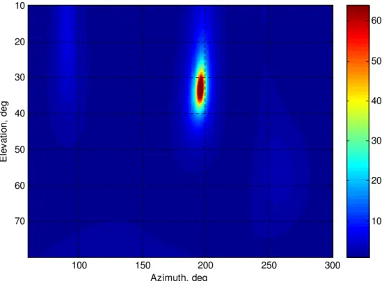
the transmitted signal for the case of two signal paths. . . 52 5.5 Incoherent integration of the CAF surfaces. . . 53 5.6 Evaluation of the (5.42) and resultant DOA (Azimuth=195.6 deg,

Elevation=32.2 deg) estimate. . . 55 5.7 Slow-time representation of the 5-element array output. (a)before

phase compensation (b)after phase compensation with the first DOA estimate. . . 57 5.8 CAF of the coherently integrated sensor outputs. . . 58 5.9 Synthetically generated copy of the first signal path on three

an-tenna output with original slow-time data. Marked lines represent the real data and smooth lines for synthetic signal. . . 60 5.10 Incoherent integration of the computed CAF surfaces of each

an-tenna output for the second path. . . 61 5.11 Proposed algorithm block diagram. . . 62

6.1 (a)Barker-13 sequence (b)One antenna output correlated with the Barker-13, a short segment. . . 65 6.2 Averaging procedure and output(κ[n]) . . . 66

(13)

6.3 rMSE of the proposed estimators as a function of the SNR for Scenario-1. (a)Azimuth θ. (b)Elevation φ. (c)Time-delay τ . (d)Doppler shift ν shift. . . 70 6.4 rMSE of the proposed estimators as a function of the SNR for

Scenario-2. (a)Azimuth θ. (b)Elevation φ. (c)Time-delay τ . (d)Doppler ν shift. . . 70

6.5 (a) 3-D and (b) 2-D spatial spectra of MUSIC algorithm. . . 71

6.6 (a) 3-D and (b) 2-D spatial spectra of CAF-DF. . . 72 6.7 rMSE of the proposed estimators as a function of the SNR for

Scenario-3. (a)Azimuth θ1. (b)Elevation φ1. (c)Time-delay τ1.

(d)Doppler shift ν1. (e)Azimuth θ2. (f)Elevation φ2.

(g)Time-delay τ2. (h)Doppler shift ν2. shift. . . 73

6.8 rMSE of the proposed estimators as a function of the SNR for

(14)

7.2 A short time segment of the actual signal at the output of an antenna element. . . 79 7.3 Map showing the path from Uppsala to Kiruna. . . 79

7.4 Incoherent integration of the CAF surfaces for the strongest path. 83

7.5 Slow-time representation of the 5-element array output. All signal amplitudes are normalized to 1. (a)before phase compensation (b)after phase compensation with the first DOA estimate. . . 84 7.6 Coherently integrated CAFs for the strongest path. . . 85 7.7 Synthetically generated copy of the strongest path at three

an-tenna output with original slow-time data. Marked lines represent the real data and smooth lines for synthetic copy signal. All signal amplitudes are normalized to 1. . . 85 7.8 Incoherent integration of the CAF surfaces for the second path. . 86 7.9 Strongest path eliminated slow-time representation of the

5-element array output. All signal amplitudes are normalized to 1. (a)before phase compensation (b)after phase compensation with the first DOA estimate . . . 87 7.10 Coherently integrated CAFs for the second path. . . 88 7.11 Synthetically generated copy of the second path at three antenna

output with original slow-time data. Marked lines represent the real data and smooth lines for synthetic copy signal. All signal amplitudes are normalized to 1. . . 88 7.12 Incoherent integration of the CAF surfaces for the third path. . . 89

(15)

7.13 Second path eliminated slow-time representation of the 5-element array output. All signal amplitudes are normalized to 1. (a)before phase compensation (b)after phase compensation with the first DOA estimate . . . 90 7.14 Coherently integrated CAFs for the third path. . . 91

7.15 Incoherent integration of the CAF surfaces for the strongest path. 92

7.16 Slow-time representation of the 5-element array output. All signal amplitudes are normalized to 1. (a)before phase compensation (b)after phase compensation with the first DOA estimate . . . 93 7.17 Coherently integrated CAFs for the strongest path. . . 94 7.18 Synthetically generated copy of the strongest path at three

an-tenna output with original slow-time data. Marked lines represent the real data and smooth lines for synthetic copy signal. All signal amplitudes are normalized to 1. . . 94 7.19 Incoherent integration of the CAF surfaces for the second path. . 95 7.20 Strongest path eliminated slow-time representation of the

5-element array output. All signal amplitudes are normalized to 1. (a)before phase compensation (b)after phase compensation with the first DOA estimate . . . 96 7.21 Coherently integrated CAFs for the second path. . . 97 7.22 Incoherent integration of the CAF surfaces for the third path . . . 98

(16)

7.23 Second path eliminated slow-time representation of the 5-element array output. All signal amplitudes are normalized to 1. (a)before phase compensation (b)after phase compensation with the first DOA estimate . . . 99 7.24 Coherently integrated CAFs for the third path. . . 100

(17)

List of Tables

6.1 Azimuth, Elevation, Delay and Doppler values of two different sce-narios in case of 1 signal path. Computational delay and Doppler resolutions are 0.1 ms and 0.0023 Hz respectively. . . 68 6.2 Azimuth, Elevation, Delay and Doppler values of four different

sce-narios in case of 2 signal paths. Computational delay and Doppler resolutions are 0.1 ms and 0.0023 Hz respectively. . . 69

7.1 Azimuth, elevation, delay and Doppler estimates of CAF-DF for 3 signal paths. Computational delay and Doppler resolutions are

0.1 ms and 0.0023 Hz respectively. . . 81

7.2 Azimuth, elevation, delay and Doppler estimates of MUSIC for 3 signal paths. Computational delay and Doppler resolutions are

7.3 Azimuth, elevation, delay and Doppler estimates of CAF-DF for 3 signal paths. Computational delay and Doppler resolutions are

7.4 Azimuth, elevation, delay and Doppler estimates of MUSIC for 3 signal paths. Computational delay and Doppler resolutions are

(18)

(19)

Chapter 1 INTRODUCTION

1.1 Objective and Contributions of this Work

Recent advances in wireless communication resulted in significant improvement in our living standards. Information transmission can be achieved via several ways by using electromagnetic, sonar, acoustic, or seismic waves as the carrier. In addition to wireless communications, radar applications also process information that bounced back from targets to deduce their position and velocity. To obtain best results, sensor arrays are widely used [1].

Compared to single sensor systems, array systems have some crucial advan-tages. First of all, for an M-sensor array, by proper processing of the received sig-nal sigsig-nal-to-noise ratio (SNR) can be increased by M times . Secondly, beams of the array can be steered freely in any desired directions. Flexible steering ability enables wireless equipment to separate multiple signals and suppress intentional or unintentional interference.

(20)

Array signal parameter estimation is a very popular research field of focus by applied statisticians and engineers as problems required ever improving per-formance. Direction of arrival (DOA) is one of the most important parameters which plays a crucial role in many real life applications. In radar, estimation of the DOA is a main issue in localization and tracking of targets. Moreover, in multi-user mobile communications, generally waves reach the receiver within a delay interval shorter than the resolution. In these cases, DOA estimates can provide spatial diversity to the receiver to enable reliable communication in multi-user scenarios [2]. Because of its importance, wide variety of algorithms have been proposed for reliable estimation of DOAs . Initial trials of signal source localization using arrays was through beamforming techniques. The idea is to form a beam in the direction of waves coming from only one particular direction. The steering directions which result in maximum signal power yields the DOA estimates [3]. Subspace methods are very well known DOA estimation techniques with high performance and relatively low computational cost. These methods basically make use of the eigen-structure of the covariance matrix of observed signals from the sensor array. The most commonly used technique in this family is the MUSIC (Multiple SIgnal Classification) technique [4, 5]. Although, mentioned approaches are very efficient in terms of computational power, they do not provide enough accuracy in correlated signal scenarios. On the otherhand, maximum likelihood (ML) techniques are highly accurate but computationally quite intensive [6, 7, 8, 9, 10]. Most recent subspace fitting methods such as signal subspace fitting (SSF) and noise subspace fitting (NSF) have the same statistical performance as the ML methods with a less computa-tional cost [11, 12, 13]. Recently, there are some efforts dealing with the DOA estimation for chirp signals by making use of ambiguity function [14, 15]. The method called AMBIGUITY-DOMAIN MUSIC (AD-MUSIC) in [14], uses the spatial ambiguity function (SAF) of the sensor array output. Once the noise subspace of the SAF matrix is estimated, the technique estimates the DOA’s

(21)

by finding the largest peaks of a localization function. In [15], details of two broadband DOA estimation methods for chirp signals based on the ambiguity function is introduced. Most of these methods take advantage of the fact that there is only a phase difference between sensor outputs, when the signals are narrowband.

Estimating the time delays and Doppler shifts of a known waveform by an array of antennas is another crucial aspect of the signal parameter estimation. For instance, in active radar and sonar, a known signal is transmitted and reflections from targets are received. The received signals are generally modeled as delayed, Doppler-shifted and scaled versions of the transmitted one. Estimation of the delay and Doppler-shift enables us to gather information about the position and the radial velocities of targets. Secondly, estimation of the parameters of the multipath communication channel, in cases where the transmitter has a rapid movement or has an unknown frequency offset, is another important application. Accurate delay and Doppler estimations are very critical in establishing a reliable communication link. Classical techniques to time-delay and Doppler estimation are based on matched filtering [16]. Matched filtering techniques are optimal for single signal arrival but are not good when multiple overlapping copies of the signal are present. In [17], a deconvolution approach for resolving multiple delayed and Doppler shifted paths where path parameters are constrained to a quantized grid is presented. Alternatively, two popular and efficient algorithms called signal subspace fitting (SSF) and noise subspace fitting (NSF), which also provide promising results when correlated signals received, can be found in [11]. In this thesis, a new signal parameter estimation technique called CAF-DF (Cross Ambiguity Function - Direction Finding) based on the cross-ambiguity function calculation will be presented. CAF-DF technique estimates DOA, time delay and Doppler shift corresponding to one of the impinging signals onto the

(22)

array in an iterative manner. Starting point of each iteration is CAF computa-tion at the output of each sensor element. Then, these 2D CAF matrixes are incoherently integrated and the largest peak on the integrated CAF is found. After that, DOA for the observed signal peak is estimated. Having found the DOA, CAF of the coherently integrated sensor outputs is computed to find ac-curate delay and Doppler estimates for the strongest signal. Then, the signal whose parameters are estimated is eliminated from the array outputs to search for the next strong signal component in the residual array outputs. Iterations continue until there is no detectable peak on the incoherently integrated CAFs. CAF-DF is different from the mentioned techniques because it both uses coherent and incoherent integration of data. It performs significantly better than the MUSIC in simulations. Especially in difficult scenarios involving low SNR and highly correlated signals, resolution capability of the CAF-DF is very promising. Moreover, there are three important differences between CAF-DF and mentioned ambiguity function based techniques [14, 15]. First of all, there isn’t any requirement to use chirp signals. Secondly, there is no need to use any other estimation technique. Lastly, CAF-DF uses cross ambiguity function instead of auto ambiguity function.

1.2 Organization of the Thesis

The organization of the thesis is as follows. In Chapter 2, a general parametric data model, which is used throughout the thesis, is introduced for sensor array systems. Then formulation and some important properties of the matched filter and ambiguity function are given. Lastly, some commonly used applications of array signal processing is presented.

In Chapter 3, spectral-based algorithmic solutions and parametric methods of DOA estimation for narrowband signals in array signal processing are presented.

(23)

In Chapter 4, basics of HF communication is introduced.The theory of wave propagation through the ionosphere is briefly discussed.

The novel DOA, delay and Doppler estimation algorithm, CAF-DF, is in-troduced in Chapter 5. Following the basic theory, detailed formulation of the CAF-DF technique is given.

The theory of an alternative MUSIC based approach proposed for HF-DF is discussed in Chapter 6. After that, simulation results and comparisons for different scenarios with the CAF-DF is presented.

Chapter 7 presents the estimated parameters of a real ionospheric data using CAF-DF and MUSIC based approach.

Finally, Chapter 8 concludes the thesis by highlighting the contributions made and list of work for future research on the subject.

(24)

Chapter 2 BASICS OF ARRAY SIGNAL

PROCESSING

The basics of array signal processing is briefly discussed in this chapter. First, underlying parametric data model for sensor arrays is introduced. Then some important points of matched filter and ambiguity function is presented. Lastly, applications of array processing are discussed.

2.1 Parametric Data Model for Sensor Arrays

Sensor arrays consists of a set of sensors that are spatially distributed at known locations with reference to a common reference point [18]. A sensor may be repre-sented as a point receiver. The propagating signals are simultaneously sampled and collected by each sensor. The source waveforms undergo some modifica-tions, depending on the path of propagation and the sensor characteristics. In this section a general parametric model will be given.

Usually, the direction and the speed of the propagation are defined by a vector

(25)

z

x

y

θ φ

.

Figure 2.1: Direction of the signal and reference coordinate system. system in Fig. 2.1, the slowness vector is

α = 1

c[cos φ cos θ ; cos φ sin θ ; sin φ] , (2.1)

where θ is the azimuth angle, φ is the elevation angle and c is the speed of light. A circular array geometry is depicted in Fig. 2.2. Position of each sensor is

represented by vector rm = [xm ; ym ; zm] = [rmsin(θm) ; rmcos(θm) ; 0] and

the propagation direction of each impinging signal is represented by unit vector

αi = (1/c)[xi ; yi ; zi], and i = 1, ..., d is the signal index. Using Eqn. 2.1, the

field measured at sensor m due to a source whose DOA is (θi, φi), can be written

as

E(rm, t) = s(t)ejw(t−ξm,i) (2.2)

where s(t) is the data signal and ξm,i is the relative phase of the mth sensor due

to ith _{impinging signal with respect to the origin of the sensor array. This phase}

(26)

z x y . Elevation Azimuth 1st impinging signal d th impinging signal Antenna element (Array sensor) m

r

) (θ ) (φ

Figure 2.2: Circular array and multipath enviroment.

ξm,i(θ, φ) = αi· rm = 1 c      cos(θi) cos(φi) sin(θi) cos(φi) sin(φi)     ·      rmcos(θm) rmsin(θm) 0      = 1 c £

rmcos(θi) cos(φi) cos(θm) + rmsin(θi) cos(φi) sin(θm)

¤

. (2.3)

In practice, before sampling takes place, the signal is down-converted to baseband which will be discussed in the following section. Therefore, without the carrier term exp(jwt), the output is modeled by

xm(t) = am(θ, φ)s(t) . (2.4)

For an M-element antenna array, the array output vector is obtained as

x(t) = a(θ, φ)s(t) . (2.5)

where a(θ, φ) is called the steering vector. Assuming a linear receiving sys-tem, if G signals impinge on an M-dimensional array from distinct DOAs

(27)

(θ1, φ1), ..., (θd, φd) the output vector takes the form x(t) = d X i=1 a(θi, φi)si(t) , (2.6)

where si(t), denote the ith baseband signal. Last equation, can be written in a

more compact form by defining a steering matrix and a vector of signal waveforms as

A(θ, φ) = £a(θ1, φ1), ..., a(θd, φd)

¤

(M ×d) (2.7)

s(t) =£s1(t); ...; sd(t)

¤

. (2.8)

Moreover, in the presence of noise n(t) we reach the well-known representation for the array input output relation;

x(t) = A(θ, φ)s(t) + n(t) . (2.9)

The signal parameters in this thesis are spatial in nature, so the following

spatial covariance matrix plays an important role:

R = E{x(t)xH_{(t)} = AE{s(t)s}H_(t)}AH _{+ E{n(t)n}H_(t)} _(2.10)

where E denotes expected value operation,

E{s(t)sH(t)} = P (2.11)

can be called source covariance matrix and

E{n(t)nH(t)} = σ2I (2.12)

is the noise covariance matrix. At all sensors we have an uncorrelated and

spa-tially white receiver noise which has variance σ2 _{and is assumed to have circularly}

(28)

In a more compact form, (2.10) can be written as R = APAH + σ2_I _(2.13) = UΛUH =£u1 . . . ud, ud+1 . . . uM ¤                µ1+ σ2 . .. µd+ σ2 σ2 . .. σ2                               uH 1 ... uH d uH d+1 ... uH M                =£Us, Un ¤  Λs+ σ2I 0 0 σ2_I    U H s UH n   = UsΛsUHs + σ2UsUHs + σ2UnUHn = UsΛsUHs + UnΛnUHn

where Λ is a diagonal matrix with real eigenvalues and U is a unitary matrix. From the equation above, it is easily seen that

APAH _{= U}

sΛsUHs . (2.14)

This says that the span of the columns of A is equal to the span of the columns

of Us (assuming that A and P are full rank). The eigenvectors associated with

the first d eigenvalues of R are the same as the eigenvectors of APAH_{. These}

eigenvectors constitute the signal subspace. The eigenvectors associated with the remaining M − d eigenvalues of R constitute the noise subspace and are orthogonal to the signal subspace.

Throughout the thesis, the number of underlying signals, d, is assumed to be known. Otherwise, we can use the techniques presented in [19, 20, 21] to estimate the number of signals impinging onto the sensor array.

(29)

2.2 Matched Filter and the Ambiguity Function

A matched filter can be defined as a type of filter matched to the known or assumed characteristics of a target signal, designed to optimize the detection of that signal in the presence of noise [22]. In the case of white additive noise, the highest SNR at the detector is obtained when the received signal is correlated with the replica of the transmitted signal. In this section, firstly complex en-velopes of the narrow bandpass signals, which make the design of the matched filter simple, will be described. After that, basics of the matched filter and how we get to the ambiguity function will be discussed.

Narrowband bandpass signals can be represented in several ways. The sim-plest one is

s(t) = g(t) cos[ωct + Φ(t)] (2.15)

where Φ(t) is the instantaneous phase and g(t) is the envelope of s(t). Second form is

s(t) = gc(t) cos(ωct) − gs(t) sin(ωct) (2.16)

where gc(t) and gs(t) are the in-phase and quadrature baseband components,

respectively, and represented as follows

gc(t) = g(t) cos(Φ(t)) (2.17)

gs(t) = g(t) sin(Φ(t)) . (2.18)

An I/Q detector, depicted in Fig. 2.3 is used to eliminate the in-phase I and the quadrature Q components using a low-pass filter which discards the high frequency terms. A third form of a narrow bandpass signal is

s(t) = Re{u(t) exp(jwct)} (2.19)

where u(t) is called the complex envelope of the signal s(t) and is defined as

(30)

) cos( 2 w_ct ) sin( 2 w_ct − )] ( cos[ ) ( ) (t g t wt t s = _c +

φ

) (t g_c ) (t g_s LPF LPF × × Figure 2.3: IQ Detector.

The angular frequency wcis called as the carrier frequency and it is significantly

larger than the bandwidth of the baseband signal. The fourth and the most general form of a narrow bandpass signal is

s(t) = 1 2u(t) exp(jwct) + 1 2u ∗_{(t) exp(−jw} ct) . (2.21)

Now we can get into the motivation and derivation of the matched filter and the ambiguity function.

Matched filters can be designed for both baseband and bandpass real signals. In the following derivations, a filter matched to the complex envelope of the signal will be considered. In Fig. 2.4, the input signal to the filter is the s(t) in

additive white gaussian noise with a two-sided power spectral density of N0/2

[22]. Impulse response of the filter is h(t) and the frequency response is H(w). The objective here is to find a h(t), which yields the maximum output SNR at a

specific t0 when we decide on the presence or absence of s(t) in white noise. The

mathematics of this objective is maximizing µ S N ¶ out = |so(t0)| 2 n2 o(t) . (2.22)

Assuming S(w) is the Fourier transform of the s(t), one can write the output of

the matched filter at t0 as

so(t0) = 1 2π Z _∞ −∞ H(w)S(w) exp(jwt0)dw (2.23)

(31)

2 / ,N₀ AWGN ) (t s s₀(t)+n₀(t) ) (t h Filter Matched +

Figure 2.4: Matched filter block diagram. The mean-squared value of the noise is

n2 o(t) = N0 4π Z _∞ −∞ |H(w)|2_dw _(2.24)

If we substitute (2.23) and (2.24) into (2.22) output SNR becomes µ S N ¶ out = ¯ ¯ ¯ Z _∞ −∞ H(w)S(w) exp(jwt0)dw ¯ ¯ ¯2 πN0 Z _∞ −∞ |H(w)|2_dw . (2.25)

Using the Schwarz inequality, (2.41) can be rewritten as µ S N ¶ out ≤ 1 πN0 Z _∞ −∞ |S(w)|2dw = 2E N0 (2.26) where E is the energy of the signal:

E = Z _∞ −∞ s2(t)dt = 1 2π Z _∞ −∞ |S(w)|2dw (2.27)

The equality in the above, Schwarz upper bound can be achieved by the following filter response which is the matched filter:

H(w) = KS∗_{(w) exp(−jwt}

0) . (2.28)

Taking the inverse fourier transform, impulse response of the filter reveals as

h(t) = Ks∗_(t

0− t) , (2.29)

meaning that delayed mirror image of the conjugate of the signal is impulse

response of the matched filter. Using this configuration, at t = t0, one can

obtain a maximum output SNR value of 2E/N0. This result is interesting in the

sense that, maximum SNR at the output of a matched filter is only a function of the signal energy but not its shape.

(32)

Let’s now investigate a filter matched to a narrowband bandpass signal. If we use the forth form of s(t), given in (2.21), in (2.23) we get the equation below:

so(t) = K

4

Z _∞

−∞

£

u(τ ) exp(jwcτ ) + u∗(τ ) exp(−jwcτ )

¤ .©u∗_{(τ − t + t} 0) exp[−jwc(τ − t + t0)] +u(τ − t + t0) exp[jwc(τ − t + t0)] ª dτ (2.30)

After straightforward simplifications, so(t) can be obtained as:

so = Re µ· 1 2K exp(−jwct0) Z _∞ −∞ u(τ )u∗_{(τ − t + t} 0)dτ ¸ exp(jwct) ¶ . (2.31)

From this long equation, we can separate out a new complex envelope:

uo(t) = 1 2K exp(−jwct0) Z _∞ −∞ u(τ )u∗_{(τ − t + t} 0)dτ , (2.32)

and in the end we obtain the output of the matched filter as

so(t) = Re

©

uo(t) exp(jwct)

ª

. (2.33)

This equation tells us that the output of a filter matched to a narrowband

band-pass signal has a complex envelope uo(t) obtained by passing the complex

en-velope u(t) of the narrowband bandpass signal through its own matched filter. Therefore, in applications where narrowband bandpass signals used, it is suffi-cient to work with the complex envelope u(t) of the signal and its matched filter

output uo(t). Once uo(t) is obtained, so(t) could be found by (2.33).

The above derivation of the matched filter ignored the potential Doppler shift on the received signals. However in wireless communication, when the receiver is moving relative to the transmitter or the received waves bounced off from moving objects, the received signal suffers a Doppler shift. When the Doppler shift is not known, performance of the receiver that makes use of a matched filter matched to the transmitted signal may significantly degrade. Now let’s modify the input complex envelope with a Doppler shift as below:

(33)

In order to find the output complex envelope we replace the first u(t) in (2.32)

by ud(t) and choose t0 = 0, K = 1 yields a function carrying both doppler shift

and time information:

uo(t, ν) =

Z _∞

−∞

u(τ ) exp(j2πντ )u∗_{(τ − t)dτ} _. _(2.35)

Another form of (2.35) is the well-known ambiguity function and given as

χ

_u,u(τ, ν) =

Z _∞

−∞

u(t)u∗(t − τ ) exp(j2πνt)dt . (2.36)

The ambiguity function (AF), characterizes the output of a matched filter when the input signal is delayed by τ and Doppler shifted by ν. This function was first introduced by Woodward in 1953 and found useful in wide variety of applications.

Let’s now mention some of the important properties of AF. If we assume that the energy E of u(t) is normalized to unity, maximum value of the ambiguity function occurs at the origin and equals to one. We can formalize it as

¯

_χ

_{(τ, ν)}¯_{¯ ≤}¯¯

_χ

_{(0, 0)}¯_{¯ = 1 .} _(2.37)

Total volume under the normalized ambiguity surface equals unity, independent of the signal waveform:

Z _∞ −∞ Z _∞ −∞ ¯ ¯

_χ

_{(τ, ν)}¯¯2 dτ dν = 1 . (2.38)

These two properties states that, if one try to squeeze the AF to a narrow peak at the origin, that peak cannot exceed a value of one and the volume squeezed out of that peak must reappear somewhere else [23]. Therefore, the behavior of the ambiguity diagram indicates that there have to be trade-offs made among the resolution, accuracy, and ambiguity. Thirdly, AF is symmetric with respect to the origin;

¯

(34)

2 ) , (τ ν χ

ν

τ

Figure 2.5: Ideal ambiguity function; ¯¯

χ

(τ, ν)¯¯2 = δ(τ, ν).

ν

τ

p

τ

/ 1 p

τ

p

τ

− p

τ

p τ

Figure 2.6: 2D view of the ambiguity function for a single pulse of width τp.

which suggests that it is sufficient to study only two adjacent quadrant of the AF.

Although it is not realistic, the “ideal” ambiguity diagram would consists of a single infinitesimal thickness peak at the origin and be zero everywhere else, as shown in Fig. 2.5. This figure tells us that we have no ambiguities in range or doppler frequency. Time delay and/or frequency could be determined simultaneously to as high a degree of accuracy as wanted.

Usually two dimensional plots of ambiguity diagrams are used to gather in-formation. In Fig. 2.6, two dimensional representation of the ambiguity diagram

(35)

for a single unmodulated pulse obtained by gating a sinusoid signal of width τp

is given. Black shaded regions indicate that ¯¯

χ

(τ, ν)¯¯2 is large and gray regions

indicate that¯¯

χ

(τ, ν)¯¯2 is small. This figure says that if τp is large corresponding

to a long pulse, we have poor delay and good doppler accuracy. The opposite occurs for a short pulse. The short pulse is doppler tolerant, meaning that the output from a filter matched to a zero doppler shift will not change much when there is a doppler shift. However, the long pulse is not doppler tolerant, and produce reduced output for a doppler-frequency shift. Lastly for this unmod-ulated pulse, the time bandwidth product (TBP) which is defined as the 3-dB timewidth times the 3-dB bandwidth of the pulse is one. For modulated pulses the TBP may significantly exceed one.

Each different waveform yields a new distribution of ambiguity. There are several types of signals that are commonly used in practice. Two important examples are the periodic continuous wave (CW) radar signal and a coherent train of identical pulses. In Fig. 2.7, ambiguity distribution of a uniform pulse

train is shown. If there are N pulses of duration τp in a pulse train where pulses

are separated by T /N, the Doppler measurement accuracy becomes 1/T which can be many time more accurate than the accuracy provided by a single pulse. This fact is illustrated in Fig. 2.7. To increase the delay accuracy, transmitted pulses can be modulated either by using phase or frequency modulations. For

example, if the pulse of duration τp is divided into 13 subpulses where the phase

of each subpulse is chosen to be {11111 − 1 − 111 − 11 − 11}, which is known as the Barker-13 sequence, the delay accuracy can be increased by 13 times. Note that, the Ambiguity distribution of a Barker-13 sequence is plotted in Fig. 2.8. The TBP of this sequence is thirteen.

(36)

ν

τ

p

τ

...

T N T / T p τ T / 1 N T / N T /

Figure 2.7: Ambiguity function distribution of an uniform pulse train.

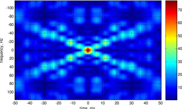
time, ms fr e q u e n c y , H z -50 -40 -30 -20 -10 0 10 20 30 40 50 -100 -80 -60 -40 -20 0 20 40 60 80 100 10 20 30 40 50 60 70

(37)

2.3 Applications of Array Processing

The practical and theoretical improvements of parameter estimation in array sig-nal processing has resulted in a many types of applications. In this section, only the three important areas, namely radar-sonar, communications and industrial applications will be discussed.

The very first application of array signal processing is in radar. Phased ar-rays are the most advanced type of antenna used in modern radars. Its a kind of array whose beam direction is controlled by the relative phases of the excitation coefficients of the relative elements [24]. Some important issues which provide radar with great flexibility can be given as: high directivity and power gain; capability of combining search and track functions when operating in multiple-target and severe interference environments; ability to change beam position in space almost instantaneously; generating very high powers from many sources distributed across the aperture; better throughput; and compatibility with dig-ital signal processing algorithms and digdig-ital computers. Furthermore, in sonar applications the signal energy is usually acoustic and measured using arrays of hydrophones. The receiving antenna usually towed under water and has the capability of detecting and locating distant sources.

Antenna arrays are extremely important in personal communications. One of the most crucial problems in a multiuser environment is the user inter-ference. This type of problems degrade the performance severely which is also the case in Code Division Multiple Access (CDMA) systems. CDMA is a form of multiplexing and a method of multiple access that does not divide up the channel by time (as in TDMA), or frequency (as in FDMA), but encodes data with a special code associated with each channel and uses the constructive interference properties of the special codes to perform the multiplexing [25]. CDMA exploits at its core mathematical properties of orthogonality. In real life applications,

(38)

varying delays of different users induce non-orthogonal codes. An implementa-tion of multiple signal classificaimplementa-tion algorithm (MUSIC), which will be discussed in Chapter 3, is presented in [26] for estimating these propagation delays. Spatial diversity had been used for a long time in order to handle the fading problem due to multipath. Nevertheless, array antennas have several additional advan-tages such as obtaining higher selectivity. For instance, a receiving array can be steered in the direction of one user at a time, while simultaneously nulling interference from other users. In [27], a similar version of the beamspace array processing describes how to localize incoming users waveforms.

In many areas of industry, array signal processing plays a central role. Medical applications are the most important commercial application areas of the sensor arrays. Circular arrays are widely used as a means to focus energy, in medical imaging and hyperthermia treatment [28]. Planar arrays are found important applications in electrocardiograms. They used to track the changes of wavefronts which in turn provide information about the situation of patient’s heart. In tomography, array signal processing used to characterize shapes of the objects [29]. Moreover, biomagnetic sensor arrays, so called super-conducting quantum interference device (SQUID) magnetometers localize brain activity [30]. Other application areas in industry may be given as; fault detection/localization and automatic monitoring. For instance, sensors are placed to detect and localize faults such as broken gears [31].

(39)

Chapter 3 DIRECTION-OF-ARRIVAL

(DOA) ESTIMATIONS

The interest in array signal processing originates from a wide range of applica-tions such as radar, radio and microwave communicaapplica-tions where waveforms are measured at several poins in space and/or time. Many estimation techniques for estimating unknown signal parameters from the measured output of a antenna array have been proposed.

Much of the current work in array signal processing has focused on meth-ods for high-resolution DOA estimation. In this chapter, well known parameter estimation techniques will be discussed in two main categories, namely

spectral-based and parametric approaches [32]. In spectral-spectral-based approaches, we form a

function of the parameter(s) of interest, e.g., the DOAs. The locations of the highest peaks of the function are considered as the DOAs estimates. Differently, in parametric techniques, we search for all parameters of interests simultaneously. In this latercase, one gets more accurate estimates however, the computational complexity also increases.

(40)

3.1 Spectral-Based Algorithmic Solutions

In the following, we will investigate the spectral-based approaches in two cate-gories: beamforming techniques and subspace-based methods.

3.1.1 Beamforming Techniques

Beamforming is a signal processing technique used with antenna arrays that controls the directionality and localize signal sources. The basic idea behind the technique is to concentrate the array to waves coming from only one particular direction. The steering directions which result in maximum signal power yields the DOA estimates. The array response can be obtained by multiplying the each sensor output with an appropriate weighting factor and forming a linear combination: y(t) = M X m=1 w∗ mxm(t) = wHxt . (3.1)

If we digitize (3.1), the output power is measured by

P (w) = 1 N N X n=1 |y(n)|2 _(3.2) = 1 N N X n=1 wHx(n)xH(n)w = wH_Rw_ˆ

where, in sample-wise notation, ˆ R = 1 N N X n=1 x(n)xH(n) (3.3) ˆ R = ˆUsΛˆsUˆ H s + ˆUnΛˆnUˆ H n .

In this thesis, two basic beamforming approaches will be investigated.

The conventional beamforming technique is the simplest one which relays on the Fourier-based spectral analysis to antenna array output [3]. The purpose is to

(41)

maximize the output power of the beamformer from a certain signal propagation direction. If the desired direction is (θ, φ), then we can write the array output as

x(t) = a(θ, φ)s(t) + n(t) . (3.4)

If we assume that the noise is spatially white, the maximum output power can be found as; max w E{w H_x(t)xH_(t)w} _(3.5) = max w w H_E{x(t)xH_(t)}w = max w {E|s(t)| 2_|wH_{a(θ, φ)|}2_{+ σ}2_|w|2_} _.

Also let |w| = 1, the maximum power can be obtained for the following choice for the w:

w = p a(θ, φ)

aH_{(θ, φ)a(θ, φ)} . (3.6)

This vector matches to the direction of impinging signal and can be thought of as a filter. If we substitute (3.6) into (3.2), the spatial spectrum is obtained as

P (θ, φ) = aH(θ, φ) ˆRa(θ, φ)

aH_{(θ, φ)a(θ, φ)} (3.7)

Conventional beamformers shows poor performance when resolving power of two sources spaced closer than a beamwidth. However, a well-known method called Capon’s beamforming proposed in [33], resolves this limitation. The cost function of the approach is introduced as

min

w P(w) (3.8)

subject to wH_{a(θ, φ) = 1} _,

which tries to minimize the power contributed by impinging signals coming from other directions than the look direction (θ, φ) and noise. One solution of (3.8) is

w = Rˆ

−1

a(θ, φ)

(42)

and the spatial spectrum is obtained by inserting the (3.9) into (3.2) as

P (θ, φ) = 1

aH_{(θ, φ) ˆ}_R−1_{a(θ, φ)} . (3.10)

This spatial spectrum and the constraint given in (3.8) gives the Capon’s beam-former the ability of better focusing in the directions where there are multiple sources.

3.1.2 Subspace-Based Methods

Spectral decomposition of a covariance matrix is the starting point of the many spectral methods in DOA analysis. Subspace-based approaches become very pop-ular with the usage of the eigen-structure of the covariance matrix. The interest was mainly due to the introduction of the MUSIC(Multiple SIgnal Classification) algorithm [4, 5].

As stated in the early sections, the spectral decomposition of a covariance matrix can be expressed as

R = APAH + σ2_I _(3.11)

= UsΛsUHs + σ2UnUHn

where the diagonal matrix Λs holds the d largest eigenvalues, assuming APAH

to be of full rank. Spatial directions of d signal sources are the solutions of the equation;

UH

na(θi, φi) = 0 (3.12)

where Un contains the noise eigenvectors.

Eigenvectors of the covariance matrix estimate, ˆR, are separated into the

signal and noise eigenvectors as in Eq.(3.3). Secondly, the orthogonal projector onto the noise subspace is found as

ˆ

Π⊥_{= ˆ}_U

nUˆ H

(43)

Then the spatial spectrum of the MUSIC algorithm is defined as

P (θ, φ) = a

H_{(θ, φ)a(θ, φ)}

aH_{(θ, φ) ˆ}_Π⊥_{a(θ, φ)} . (3.14)

Performance of the MUSIC algorithm is significantly better than the beam-forming techniques and provides statistically consistent estimates. However, at low SNR and closely spaced signals scenarios , MUSIC fails to resolve DOAs. This resolution loss is more revealed for highly correlated signals. In the case of coherent signals, Eqn.(3.12) becomes false and the algorithm fails to yield consistent estimates.

The idea behind the MUSIC algorithm is applied to many application areas and led to a multiple of variants. One of the most successful variant is the

weighted MUSIC, which has a spatial spectrum as P (θ, φ) = a

H_{(θ, φ)a(θ, φ)}

aH_{(θ, φ) ˆ}_Π⊥_{W ˆ}_Π⊥_{a(θ, φ)} . (3.15)

The effects of the eigenvectors are taken into account through the weighting matrix W. Although uniform weighting usage yields estimates with minimal variance, in some scenarios involving correlated signals, low SNR and short du-ration signals, a non-uniform weighting improve the resolution of the algorithm considerably with an acceptable increase in the variance [34].

3.2 Parametric Methods

Spectral-based methods discussed in the previous section are very effiecient in terms of computational power. However, they do not provide enough accuracy for different cases. For instance, in correlated signal scenarios, performance of the spectral-based algorithms degrades significantly. Parametric methods fill the gap in coherent signal DOA estimations. These methods provide better accu-racy and robustness but at the same time require a multidimensional search to

(44)

produce estimates. In this section, deterministic maximum likelihood, stochastic likelihood and subspace-based approximations will be discussed respectively.

3.2.1 Deterministic Maximum Likelihood

In our data model, we assume that the signal carrying the data is emitted from d sources whereas background and receiver noise can be thought of as emanating from a large number of independent sources. As a result, data signals are deter-ministic and noise is assumed to be a stationary Gaussian white random process [32].

In the case of spatially white and circularly symmetric noise, statistical prop-erties can be written as

E{n(t)nH_{(t)} = σ}2_I _(3.16)

E{n(t)nT_{(t)} = 0} _. _(3.17)

By means of the assumptions above, array output x(t) can be modeled as circu-larly symmetric and temporally white Gaussian random process having a mean

A(θ, φ)s(t) and covariance σ2_{I. The probability density function (PDF) of x(t)}

is the complex L-variate Gaussian: 1

(πσ2₎L/2 e

−kx(t)−As(t)k2_/2σ2

, (3.18)

where k.k denotes the Euclidean norm. Measurements are independent so likeli-hood function is given as

L(θ, φ, s(t), σ2) = N Y t=1 1 (πσ2₎L/2 e −kx(t)−As(t)k2_/2σ2 . (3.19)

Direction of arrivals (θ, φ), signal waveforms s(t), and the noise variance σ2

are the parameters that should be estimated. Calculated ML estimates of these

(45)

likelihood function: l(θ, φ, s(t), σ2_{) = L log σ}2₊ 1 σ2_N N X t=1 kx(t) − As(t)k2 _(3.20)

is commonly used. The minimizing arguments of the log likelihood function are called as the deterministic maximum likelihood (DML) estimates. Note that the

DML estimates for σ2 _{and s(t) are:}

where A† _{is the pseudo inverse of A and ˆ}_{R is the sample covariance matrix}

[35, 7].

If we substitute (3.21) and (3.22) into (3.19), the DML estimates for θ and φ can be expressed as:

ˆ

θ tr

©

(I − AA†) ˆRªª (3.23)

In order to obtain ˆθ and ˆφ, one should solve the non-linear d-dimensional

opti-mization problem. Good initial estimates lead to very accurate DOA estimates. However, as stated before computational complexity is very high.

3.2.2 Stochastic Maximum Likelihood

Stochastic maximum likelihood (SML) method is derived by modeling the signal waveforms as Gaussian random processes. By [8, 9], the accuracy of the parame-ter estimates are related with correlations and power of the waveforms. Assume that, some properties of the signal is given as

(46)

saying that x(t) is a white, zero-mean and circularly symmetric gaussian random vector having a covariance matrix

R = A(θ, φ)PAH(θ, φ) + σ2I . (3.26)

where the unknown parameters are (θ, φ), P and σ2_.

and for fixed θ, φ, the minimum with respect to σ2 _{and P can be given as [10]}

σ2(θ, φ) = 1 M − dtr{Π ⊥ A} (3.28) ˆ P(θ, φ) = A†¡R − ˆˆ σ2_{(θ, φ)I}¢_A†H _. _(3.29)

If we substitute (3.28) and (3.29) into (3.27), we get the following expression for the SML estimates of θ and φ:

ˆ

θ log

¯

¯A ˆP(θ, φ)AH_{+ ˆ}_σ2_{(θ, φ)I}¯_¯ª _. _(3.30)

SML parameter estimates are better than the DML estimates in low SNR and highly correlated signal situations. Moreover, this method provides robust results even if the distribution of the signal waveform is not Gaussian.

3.2.3 Subspace-Based Approximations

We already mentioned that, conventional beamforming techniques are signifi-cantly behind the subspace-based methods as far as the performance and the accuracy are our concern. Moreover, in uncorrelated signal scenarios, MUSIC performs identical to DML in accuracy [34]. However, resolution problems occur for finite samples and high source correlation scenarios in spectral-based meth-ods. In this section, some well-known Subspace Fitting methods, which offer

(47)

the same statistical performance and are computationally very efficient, will be discussed.

Let’s restate the eigendecomposition of the array covariance matrix (3.11),

R = APAH + σ2_I _(3.31)

= UsΛsUHs + σ2UnUHn . (3.32)

We know that if P is a full rank matrix, then A and Us span the same range

space. However, in general, the rank of P is ˜d which is the number of eigenvectors

in Us. Then Us will span a ˜d-dimensional subspace of A. Since,

I = UsUHs + UnUHn (3.33)

we have the following equality

APAH + σ2_U

sUHs = UsΛsUHs . (3.34)

After some simple manipulations on the equation above we obtain:

Us = AT (3.35)

where T is the full rank ( ˜d) matrix given by

T = PAH_U s ¡ Λs− σ2I ¢₋₁ . (3.36)

Equation (3.35) is the basic starting point of the Signal Subspace Fitting

(SSF) approach [12, 6]. In order to solve the (3.35) one needs a search for the

unknown parameters (θ, φ) and T. Obviously, resulting (θ, φ) are the DOAs. If

instead of Us, an estimate ˆUs is used then the distance between the ˆUs and

AT should be minimized. The SSF estimates are found by solving the following optimization problem: ©_ˆ θ, ˆφ, ˆTª = arg min θ,φ,T ° ° ˆ_U_s_{− AT}°°2 F . (3.37)

For fixed but unknown A, the estimate of T is ˆ

(48)

and using this result, the required optimization can be expressed as: ˆ θ, φ = arg©min θ,φ © Π⊥ AUˆsΛ ˆˆU H s ªª (3.39)

Another form of a subspace fitting approach is obtained by using the following equation;

AH(θ, φ)Un = 0 , (3.40)

which holds for P having full rank. After an estimate of Un is found, signal

parameters can be determined by minimizing the following equation; ˆ θ, ˆφ = arg©min θ,φ tr © AHUˆnUˆ H nAV ªª , (3.41)

which is known as noise subspace fitting (NSF) criterion [6, 13]. In this equation V is a positive definite weighting matrix. For V = I and in the case of |a(θ, φ)| is independent of (θ, φ), this method reduces the MUSIC algorithm. The criterion function is a quadratic function of the steering matrix A. If any of the parameters of A enter linearly then it is very easy to obtain an analytical solution with respect to these variables [36]. However, NSF fails to produce reliable estimates in coherent signal situations [11, 32].

(49)

Chapter 4 HF COMMUNICATION

Modern radio technology actually starts with the publication of James Clerk Maxwell’s Treatise on Electricity and Magnetism in 1873, introducing the basic theory of electromagnetic wave propagation. However, the first radio waves were actually detected 15 years later. In 1888, Heinrich Rudolph Hertz showed that disturbances generated by a spark coil showed the characteristics of Maxwell’s radio waves. His work impressed Guglielmo Marconi’s early experiments with wireless telegraphy using Morse code. By 1896, Marconi had communicated messages over distances of a few kilometers.

In those years, it was thought that radio waves in the atmosphere traveled in straight lines and that they therefore would not be useful for over-the-horizon communication. However, Marconi achieved radio communication over long dis-tances. In 1901 in Newfoundland, Canada, he detected a telegraphic signal transmitted from Cornwall, England,3000 kilometers away using a 120 meters long wire.

Marconi’s achievement activated a huge effort on this issue. Eventually Ed-ward Appleton answered the question of how radio waves could be received around the surface of the earth. He discovered that a blanket of electrically

(50)

charged, or ”ionized”, particles in the earth’s atmosphere, the ”ionosphere”, were capable of reflecting radio waves. By the 1920s, researchers had used this theory and developed ways to predict the refractive properties of the ionosphere. Today, with the experience and understanding of the propagating effects of the ionosphere, HF technology provides reliable and effective communication over many thousands of miles. In this chapter, structure and some important prop-erties of this natural satellite will be discussed.

4.1 Structure of the Ionosphere

The ionosphere is composed of a number of ionised regions above the earth’s atmosphere, which extends from a height of about 60 km to 600 km. These regions are believed to influence the radio waves mainly because of the presence of free electrons, which are arranged in approximately horizontally stratified layers [37].

The ionisation in the ionosphere is caused mainly by radiation from the sun. This is a process by which electrons, having a negative charge, are stripped from the neutral atoms or molecules to form positively charged ions. It is these ions that give their name to the ionosphere. These electrons under the influence of an electromagnetic wave will absorb and reradiate energy, and modify direction of an electromagnetic wave.

Most of the ionisation in the ionosphere results from ultraviolet light, although this does not mean that other wavelengths do not have some effect. Addition-ally, each time an atom or molecule is ionised, a small amount of energy is used. This means that as the radiation passes further into the atmosphere, its intensity reduces. It is for this reason that the ultraviolet radiation causes most of the ionisation in the upper reaches of the ionosphere, but at lower altitudes the radi-ation that is able to penetrate further cause more of the ionisradi-ation. Accordingly,

(51)

Solar radiation

Uncharged molecule

Positively charged ion Free electron

Figure 4.1: Electron production due to solar radiation.

extreme ultra-violet and X-Rays give rise to most of the ionisation at lower alti-tudes. In addition to this, there is a variation in the proportions of monatomic and molecular forms of the gases, the monatomic forms of gases being far greater at higher altitudes. These and a variety of other phenomena mean that there are variations in the level of ionisation with altitude.

The level of ionisation in the ionosphere also changes with time. It varies with the time of day, time of year, and according to many other external influences. One of the main reasons why the electron density varies is that the sun, which gives rise to the ionisation. While the radiation from the sun causes the atoms and molecules to split into free electrons and positive ions. The reverse effect also occurs. When a negative electron meets a positive ion, the fact that dissimilar charges attract means that they will be pulled towards one another and they may combine. This means that two opposite effects of splitting and recombination are taking place. This is known as a state of dynamic equilibrium. Accordingly the level of ionisation is dependent upon the rate of ionisation and recombination.

(52)

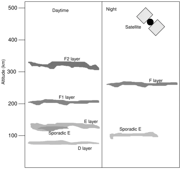
100 200 300 400 500 F2 layer F1 layer E layer Sporadic E D layer F layer Sporadic E Satellite Daytime Night A lt it u d e ( k m )

Figure 4.2: Ionosphere layers.

4.2 Layers of Ionosphere

The ionosphere is often described in terms of its component regions or layers which are firstly mentioned by E.V. Appleton. Naming convention were based upon data obtained from a myriad of radiowave measurement schemes involving vertical and oblique geometries, pulsed and CW systems, variable and constant frequencies, and different types of observables such as polarization and signal time delay [38]. For reasons related to historical development of ionospheric research, the ionosphere is divided into three regions or layers designated D,E and F respectively, in order of increasing altitude. The D layer is the innermost layer, within the ionosphere that affects radio signals to any degree. It is present

(53)

at altitudes between about 60 and 90 kilometres and the radiation within it is only present during the day to an extent, which affects radio waves noticeably. It is sustained by the radiation from the sun and levels of ionisation fall rapidly when the sun sets. In this region, electron density, which has a maximum value shortly after local solar noon and a very small value at night, exhibits large diurnal variations. The D layer mainly has the affect of absorbing or attenuating radio signals particularly LF and MF slice of the radio spectrum. At night it has little effect on most radio signals.

The altitude range from 90 - 130 kilometres constitutes the E-region and en-compasses the so-called ‘normal’ and sporadic E layers. The former is a regular layer which displays a strong solar zenith angle dependence with maximum den-sity near noon and important only for daytime HF propagation. Sporadic E may form at any time during the day or night. It is difficult to know where and when it will occur and how long it will persist. Sporadic E can have a comparable electron density to the F region. This means that it can refract comparable fre-quencies to the F region. Sometimes a sporadic E layer is transparent and allows most of the radio wave to pass through it to the F region, however, at other times the sporadic E layer obscures the F region totally and the signal does not reach the receiver which is known as sporadic E blanketing. Sporadic E in the low and mid-latitudes occurs mostly during the daytime. At high latitudes, it generally forms at night.

The most important region in the ionosphere for long distance HF commu-nications is the F region. It extends upwards from about 135 kilometres and is divided into the F1 and F2 layers during the daytime when radiation is being received from the sun. Typically the F1 layer is found at around an altitude of 180 kilometres with the F2 layer above it at around 350 kilometres. The F1 layer exists only during daylight and is sometimes the reflecting region of the HF transmission. However, generally obliquely-incident waves that penetrate the E

(54)

region also penetrate the F1 layer and are reflected by the F2 layer. At night, F1 layer merges with the F2 layer at a height of about 300 kilometres [37]. Prin-cipal reflecting region for long distance HF communication is the F2 layer since it provides us with the capability to achieve the greatest skywave propagation range (by a single hop) at generally the highest allowable frequency in relation to underlying layers. The lifetime of electrons is greatest in the F2 layer which is one reason why it is present at night.

4.3 Wave Propagation through the Ionosphere

In an earth environment, electromagnetic waves propagate in ways that depend not only on their own properties but also on those of the environment itself. Waves travel in straight lines, except where the earth and the atmosphere alter their path. Waves with frequencies above HF travel in a straight line. They propagate by means of so-called space waves. They are sometimes called tropo-sphereic waves, since they travel in the troposphere. Frequencies below the HF range travel around the curvature of the earth. They are called ground waves or surfaces waves. Waves in the HF range are reflected by the ionised layers of the atmosphere and are called sky waves. Such signals are beamed into the sky and come down again after reflection, returning to earth well beyond the horizon. In this section, having mentioned the structure and the layers of the ionosphere, we will focus on how and in what conditions wave propagation through the iono-sphere enables HF communication.

Using the optimum operational frequency is very crucial in HF communica-tion. Not all HF waves are refracted by the ionosphere, saying that there are upper and lower frequency bounds for communication between two stations. The range of usable frequencies will change through out the day, with the seasons, from place to place and with the solar cycle. If the frequency is too low, the

A novel array signal processing technique for multipath channel parameter estimation

A NOVEL ARRAY SIGNAL PROCESSING

TECHNIQUE FOR MULTIPATH CHANNEL

PARAMETER ESTIMATION

a thesis

submitted to the department of electrical and

electronics engineering

and the institute of engineering and sciences

of bilkent university

in partial fulfillment of the requirements

for the degree of

master of science

By

Mehmet Burak G¨uldo˘gan

July 2006

ABSTRACT

A NOVEL ARRAY SIGNAL PROCESSING

TECHNIQUE FOR MULTIPATH CHANNEL

PARAMETER ESTIMATION

Mehmet Burak G¨uldo˘gan

M.S. in Electrical and Electronics Engineering

Supervisor: Prof. Dr. Orhan Arıkan

July 2006

¨

OZET

C

¸ OKLUYOL KANAL PARAMETRE KEST˙IR˙IM˙I ˙IC

¸ ˙IN YEN˙I

B˙IR D˙IZ˙I S˙INYAL ˙IS¸LEME TEKN˙I ˘

G˙I

Mehmet Burak G¨uldo˘gan

Elektrik ve Elektronik Mühendisli¯gi Bölümü Yüksek Lisans

Tez Y¨oneticisi: Prof. Dr. Orhan Arıkan

Temmuz 2006

ACKNOWLEDGMENTS

Contents

List of Figures

χ

List of Tables

Chapter 1

INTRODUCTION

1.1

Objective and Contributions of this Work

1.2

Organization of the Thesis

Chapter 2

BASICS OF ARRAY SIGNAL

PROCESSING

2.1

Parametric Data Model for Sensor Arrays

r

2.2

Matched Filter and the Ambiguity Function

φ

χ

χ

χ

χ

ν

τ

χ

ν

τ

τ

τ

τ

τ

χ

χ

ν

τ

τ

...

2.3

Applications of Array Processing

Chapter 3

DIRECTION-OF-ARRIVAL

(DOA) ESTIMATIONS

3.1

Spectral-Based Algorithmic Solutions

_χ

_χ

_χ